exitvoice appendix 最近の更新履歴 Takashi SHIMIZU

Cheap Talk with an Exit Option:

A Model of Exit and Voice:

Online Appendix

Takashi Shimizu^∗ Jamuary 2017

A Necessity of Receiver’s Exit Aversion

In the next section, we derive the conditions for equilibria including those other than NEEs. In this section, we draw a rough sketch and show that R’s exit aversion is necessary for the credibility of exit to serve for the informative communication.

Given any equilibrium interval ˆτ where inf ˆτ = t, sup ˆτ = t, and ˆa = α◦ µ(t) for t ∈ ˆτ. Then, ˆτ belongs to either Intervals N , A, F or any one of the following categories:¹

• Interval R:

* t− t > −b +^√DS+√DR,

* ˆa = t +^√D^R,

* y^S(t, ˆa) > U^S

* y^S(t, ˆa) < U^S, and

∗Graduate School of Economics, Kobe University, 2-1 Rokkodai-cho Nada-ku, Kobe, 657-8501 JAPAN (e-mail: shimizu@econ.kobe-u.ac.jp)

1In taking all kinds of equilibria into consideration, the length constraint on Interval A should be modified as follows:

2^√D^S− 2b ≤ t − t < min{2^√DS,−b +^√DS+√DR}. Note that the condition^√D^R_≥^√D^S+ b which appears in Lemma 2 implies that

2^√D^S_{≤ −b +}^√D^S+^√D^R.

* S exercises the exit option on the right side of the interval.

• Interval B:

* t_{− t > 2}^√D^S,

* ˆa_{∈ [t + b +}^√D^S, t + b₋^√D^S],

* y^S(t, ˆa)_{≤ U}^S where the equality holds only if ˆa = t + b +^√D^S,

* y^S(t, ˆa)_{≤ U}^S where the equality holds only if ˆa = t + b₋^√D^S , and

* S exercises the exit option around either end of the interval; in particular, S does so around both ends of the interval when ˆa_{∈ (t + b +}^√D^S, t + b₋^√D^S).

• Interval E:

* there is no constraint for the length of interval,

* ˆa∈ (−∞, t + b −^√DS]∪ [t + b +^√DS,∞),

* y^S(t, ˆa)_{≤ U}^S where the equality holds only ˆa = t + b₋^√D^S,

* y^S(t, ˆa)_{≤ U}^S where the equality holds only if ˆa = t + b +^√D^S ,and

* S almost always exercises the exit option in this interval.

In any type of the intervals listed here, S necessarily exercises the exit option at some states. For example, when^√D^R_{≤ b −}^√D^S (Case 8), R intentionally induces S to exercise the exit option by choosing ˆa∈ (−∞, t + b −^√DS]∪ [t + b +^√DS,∞) such that S’s stay payoff becomes sufficiently small compared to his exit payoff.

Also, in Section B, we completely enumerate the possible equilibrium intervals and the possible connections of them, which enable us to check whether a given configuration of intervals constitutes an equilibrium. Using these, we investigate equilibria when D^Ris not so large and demonstrate that R’s aversion to S’s exit is necessary for the credibility of exit to serve for the informative communication.

First, when ^√D^R<^√D^S+ b, possible NEE configurations are restricted as follows:

• N . . . N

• N . . . N A

• A

This means that the condition ^√D^R _≥ ^√D^S + b, which is the sufficient condition for Theorem 1, is also necessary for the existence of informative NEE driven by the credibility of exit.

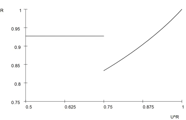
Moreover, we demonstrate that an increase in R’s exit payoff can lead to a decrease in her equilibrium payoff. Consider the case in which b = ^√D^S = ¹₄, and Y^R = 1. In this case, as the value of U^R changes, the equilibrium outcome changes as follows:

• When U^R ≤ ³₄ (Case 2), a configuration FF constitutes an equilibrium. It gives R the ex ante expected equilibrium payoff V^R= ¹¹₁₂.

• When ³₄ ^{< UR}< 1 (Case 4), only a configuration R constitutes an equilibrium.^{2 It} gives R the ex ante expected equilibrium payoff V^R as follows:

V^R= U^R₋

∫

√D^R 0

(t₋^√D^R)²dt + D^R√D^R.

V^R is illustrated in Figure 1. It is obvious that it has a downward jump at U^R= ³₄. This means that an increase in U^R reduces her equilibrium payoff.

<Figures 1 should be inserted>

Let us see what happens in more detail. When U^R_≤ ³₄, the following strategy profile constitutes an equilibrium:

• the state space is partitioned into [0,¹₂^{) and [1}₂^{, 1],}

• S informs R of which interval the realized state is lying on,

• when R is informed that t ∈ [0,¹₂), she chooses a = ¹₂, and

• when R is informed that t ∈ [¹₂, 1], she chooses a = 1.

In this equilibrium, R attempts to deter S from exercising the exit option as she is averse to exit. Fix the strategy profile and suppose that U^R becomes more than ³₄. R then does no longer do her best to stop S’s exit. To be more concrete, her best response is

{1

4 if she is informed that t∈ [0, 1/2),

3

4 if she is informed that t∈ [1/2, 1].

2Since 1 > 2^√D^S, a configuration A cannot constitute an equilibrium.

This response induces S to choose the exit option on the right side of each interval. Given this response, S is no longer indifferent between sending messages corresponding to those two intervals on the boundary state t = ¹₂. For, if she sends the message indicating t_{∈ [0,}¹₂), then

y^{S( 1} 2^,

1 4

)

= Y^S₋¹ 4 ^{< Y}

S₋ ¹

16 ^{= U}

S_,

and therefore, S exercises the exit option and obtains a payoff of U^S. On the other hand, if she sends the message indicating t_{∈ [}¹₂, 1], then

y^{S( 1} 2^,

3 4

)

= Y^S> Y^S₋ ¹ 16 ^{= U}

S_,

and therefore, she chooses to stay and obtains a payoff of Y^S, which is strictly larger than U^S. It then follows that such an information transmission cannot sustain as an equilibrium outcome. On the whole, an increase in R’s exit payoff deteriorates the informativeness of equilibrium communication, which in turn reduces her equilibrium payoff.

This is not an irregular outcome. Indeed, we can show that a similar outcome would happen whenever^√D^S _{≤ b and}^√D^S _≤ ¹₄. All in all, we conclude that R’s exit aversion is necessary for the credibility of exit to serve for the informative communication.

B Characterization of General Equilibria

In this section, we derive the conditions for equilibria including those other than no-exit equilibria.

We assume D^S > 0 and D^R > 0 throughout this section. First of all, S’s optimal exit strategy is as follows:

ϵ(t, a) =

{0 if a_{− b −}^√D^S ≤ t ≤ a − b +^√DS, 1 otherwise.

Next, we consider R’s best response. Fix an interval τ where inf τ = t and sup τ = t. Suppose R is informed via cheap S’s message that a realized state t is lying on the interval τ . Denote R’s expected equilibrium payoff on choosing a conditional on the belief that t_{∈ τ by ˜}V^R(a) and, for ease of exposition, define W (a) = (t_{− t)( ˜}V^R(a)_{− U}^R), which is written as follows:

Case 1: t_{− t ≤ 2}^√D^S W (a) =



















0 if a_{∈ A}¹₁:= (−∞, t + b −^√DS],

(a_{− b +}^√D^S_{− t)D}^R₋^∫a−b+

√D^S

t ^{(t− a)2dt if a∈ A1}2^{:= [t + b}−^{√DS, t + b}−^√DS], (t_{− t)D}^R₋^∫_t^t(t_{− a)}²dt if a_{∈ A}¹₃:= [t + b₋^√D^S, t + b +^√D^S], (t_{− a + b +}^√D^S)D^R₋^∫_a^t_−b−^√_DS(t_{− a)}²dt if a_{∈ A}¹₄:= [t + b +^√D^S, t + b +^√D^S],

0 if a_{∈ A}¹₅:= [t + b +^√D^S,_∞).

Case 2 : t_{− t > 2}^√D^S W (a) =



















0 if a_{∈ A}²₁:= (−∞, t + b −^√DS],

(a_{− b +}^√D^S_{− t)D}^R₋^∫a−b+

√D^S

t ^(t− a)^{2dt if a}∈ A²2^{:= [t + b}−^{√DS, t + b +√DS],} 2^√D^SD^R₋^∫a−b+

√D^S a_−b−^√D^{S(t− a)}

2_{dt if a∈ A}2

3:= [t + b +^√D^S, t + b₋^√D^S], (t_{− a + b +}^√D^S)D^R₋^∫_a^t_−b−^√_DS(t_{− a)}²dt if a_{∈ A}²₄:= [t + b₋^√D^S, t + b +^√D^S],

0 if a_{∈ A}²₅:= [t + b +^√D^S,_∞).

By tedious calculation, we obtain the following result: Lemma B.1 We define

aⁱ_j = arg max

a_∈Aⁱ_j

W (a).

Then, a¹₁ = A¹₁, a¹₅ = A¹₅, a²₁= A₁², a²₃= A²₃, a²₅= A²₅. And as for a¹₂;

• If b <^√DS− 2^{√DR, then}

a¹₂ =_{{t + b −}^√D^S_}.

• If b =^√DS− 2^{√DR, then} a¹₂ =

{{t + b −^√DS} ^{if t}− t < −b +^√DS+√DR, {t +^{√DR, t + b}−^√DS} ^{if t}− t ≥ −b +^√DS+√DR.

• If^√DS− 2^√DR< b <^√D^S+^√D^R, then a¹₂ =

{{t + b −^√DS} ^{if t}− t ≤ −b +^√DS+√DR, {t +^√DR} ^{if t}− t ≥ −b +^√DS+√DR.

• If b ≥^{√DS+√DR, then}

a¹₂ =_{{t + b −}^√D^S_}. As for a¹₃;

a¹₃= {{_t+t

2

} if t_{− t ≤ 2}^√D^S_{− 2b,} {t + b −^√DS} ^{if t}− t ≥ 2^√DS− 2b. As for a¹₄;

• If b +^√DS ≤^{√DR, then} a¹₄ =

{{t + b +^√DS} ^{if t}− t ≤ b +^√DS+√DR, {t −^√DR} ^{if t}− t ≥ b +^√DS+√DR.

• If^{√DR< b +√DS< 2√DR, then}

a¹₄ =























{t + b +^√DS} ^{if t}− t < ^3(b+

√D^S₎₋^√12D^R_−3(b+^√D^S)²

2 ^,

{t + b +^{√DS, t + b +√DS}} ^{if t}− t = ^3(b+

√D^S₎₋^√12D^R_−3(b+^√D^S)²

2 ^,

{t + b +^√DS} ^{if 3(b+}

√D^S₎₋^√12D^R_−3(b+^√D^S)² 2

< t_{− t ≤ b +}^√D^S+^√D^R, {t −^√DR} ^{if t}− t ≥ b +^√DS+√DR.

• If b +^{√DS = 2√DR, then} a¹₄ =

{{t + b +^√DS} ^{if t}− t < ³₂^{(b +√DS),} {t + b +^{√DS, t}−^√DR} ^{if t}− t ≥ ³₂^{(b +√DS).}

• If b +^{√DS > 2√DR, then}

a¹₄ =_{{t + b +}^√D^S_}. As for a²₂;

• If^{√DS <√DR, then}

a²₂ =







{t + b +^√DS} ^{if b}≤ −^√DS+√DR,

{t +^√DR} ^if −^√DS+√DR≤ b ≤^√DS+√DR, {t + b −^√DS} ^{if b}≥^√DS+√DR.

• If^√DR≤^√DS≤ 2^{√DR, then}

a²₂ =

{{t +^√DR} ^{if b}≤^√DS+√DR, {t + b −^√DS} ^{if b}≥^√DS+√DR.

• If^{√DS > 2√DR, then}

a²₂ =















{t + b −^√DS} ^{if b <√DS}− 2^√DR, {t + b −^{√DS, t +√DR}} ^{if b =√DS}− 2^√DR,

{t +^√DR} ^if√DS− 2^{√DR< b}≤^√DS+√DS, {t + b −^√DS} ^{if b}≥^√DS+√DR.

As for a²₄;

• If^√DS ≤^{√DR, then}

a²₄ =











{t + b −^√DS} ^{if b <}

√

−^D₃^{S + DR,} {t + b −^{√DS, t + b +√DS}} ^{if b =}

√

−^D₃^{S + DR,} {t + b +^√DS} ^{if b >}

√

−^D₃^{S + DR.}

• If^{√DR<√DS< 3}₂^{√DR, then}

a²₄ =















{t −^√DR} ^{if b}≤^√DS−^√DR, {t + b −^√DS} ^if√DS−^√DR≤ b <

√

−^D₃^{S + DR,} {t + b −^{√DS, t + b +√DS}} ^{if b =}

√

−^D₃^{S + DR,} {t + b +^√DS} ^{if b >}

√

−^D₃^{S + DR.}

• If ³₂^√DR≤^{√DS< 2√DR, then}

a²₄ =







{t −^√DR} ^{if b <}−^{√DS+ 2√DR,} {t −^{√DR, t + b +√DS}} ^{if b =}−^{√DS+ 2√DR,} {t + b +^√DS} ^{if b >}−^{√DS+ 2√DR.}

• If^√DS ≥ 2^{√DR, then a2}4 ⁼{t + b +^√DS} .

In order to characterize R’s best response, the following lemma is necessary:

Lemma B.2 Suppose b < ^√D^S₋^√D^R and _{−b +}^√D^S+^√D^R < t_{− t < 2}^√D^S _{− 2b.} Then, there exists ˆT such that ˆT _{∈ (−b +}^√D^S+^√D^R, 2^√D^S_{− 2b) and}

W^{( t + t} 2

)







>

=

<







W (t +^√D^R) _{⇔ t − t}







<

=

>





 T .ˆ

Moreover, such ˆT is unique.

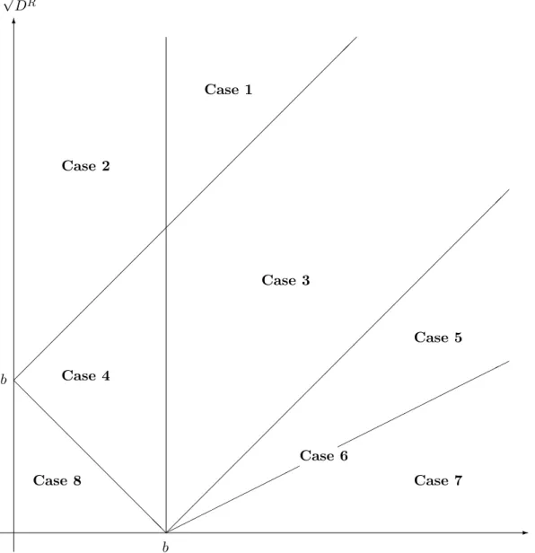
Now we are in a position to completely characterize R’s best response. Proposition B.1 Let

AE := A¹_{1∪ A}¹₅= A²_{1∪ A}²₅. Then, Receiver’s best response a^∗ is as follows:

Case 1: b <^√D^S and b_{≤ −}^√D^S+^√D^R

a^∗ =









 {t+t

2

}

if t_{− t < 2}^√D^S_{− 2b,}

{t + b −^√DS} ^{if 2√DS}− 2b ≤ t − t ≤ 2^√DS, A²₃ if t_{− t > 2}^√D^S.

Case 2: ^√D^S_{≤ b ≤ −}^√D^S+^√D^R a^∗=

{{t + b −^√DS} ^{if t}− t ≤ 2^√DS, A²₃ if t_{− t > 2}^√D^S. Case 3: ₋^√D^S+^√D^R< b <^√D^S and b_≥^√D^S₋^√D^R

a^∗ =









 {t+t

2

} if t_{− t < 2}^√D^S_{− 2b,}

{t + b −^√DS} ^{if 2√DS}− 2b ≤ t − t ≤ −b +^√DS+√DR, {t +^√DR} ^{if t}− t > −b +^√DS+√DR.

Case 4: ₋^√D^S+^√D^R< b <^√D^S+^√D^R and b_≥^√D^S a^∗ =

{{t + b −^√DS} ^{if t}− t ≤ −b +^√DS+√DR, {t +^√DR} ^{if t}− t > −b +^√DS+√DR.

Case 5: ^√D^S_{− 2}^√D^R< b <^√D^S₋^√D^R

a^∗=









 {t+t

2

} if t_{− t < ˆ}T , {t+t

2 ^{, t +}

√D^R} if t_{− t = ˆ}T , {t +^√DR} ^{if t}− t > ˆ^{T .} Case 6: b =^√D^S_{− 2}^√D^R

a^∗ =









 {t+t

2

}

if t_{− t <}^√12D^R, {t+t

2 ^{, t +}

√D^R}_{∪ A}E if t_{− t =}^√12D^R, {t +^√DR} ∪ A^{E if t}− t >^√12DR. Case 7: b <^√D^S_{− 2}^√D^R

a^∗ =









 {t+t

2

} if t_{− t <}^√12D^R, {t+t

2

}∪ AE if t_{− t =}^√12D^R, AE if t_{− t >}^√12D^R.

Case 8: b_≥^√D^S+^√D^R

a^∗= AE.

These cases are illustrated in Figure 2.

<Figures 2 should be inserted>

Based on R’s response, candidates for equilibrium intervals can be classified into the following the six categories (where ˆa = α◦ µ(t) for t ∈ τ):

• Interval N :

* t_{− t < 2}^√D^S_{− 2b,}

* ˆa = ^t+t₂ ,

* y^S(t, ˆa) > U^S,

* y^S(t, ˆa) > U^S, and

* S never exercises the exit option in this interval.

• Interval A:

* 2^√D^S− 2b ≤ t − t < min{2^√DS,−b +^√DS+√DR},

* ˆa = t + b₋^√D^S,

* y^S(t, ˆa) > U^S,

* y^S(t, ˆa) = U^S, and

* S never exercises the exit option in this interval.

• Interval F:

* t_{− t = 2}^√D^S,

* ˆa = t + b₋^√D^S,

* y^S(t, ˆa) = y^S(t, ˆa) = U^S, and

* S never exercises the exit option in this interval.

• Interval R:

* t− t > −b +^√DS+√DR,

* ˆa = t +^√D^R,

* y^S(t, ˆa) > U^S

* y^S(t, ˆa) < U^S, and

* S exercises the exit option on the right side of the interval.

• Interval B:

* t_{− t > 2}^√D^S,

* ˆa_{∈ A}²₃,

* y^S(t, ˆa)_{≤ U}^S where the equality holds only if ˆa = t + b +^√D^S,

* y^S(t, ˆa)_{≤ U}^S where the equality holds only if ˆa = t + b₋^√D^S , and

* S exercises the exit option around either end of the interval. Particularly, S does so around both ends of the interval when ˆa_{∈ int A}²₃.

• Interval E:

* there is no constraint on the length of interval,

* ˆa_{∈ A}E,

* y^S(t, ˆa)_{≤ U}^S where the equality holds only ˆa = t + b₋^√D^S,

* y^S(t, ˆa)_{≤ U}^S where the equality holds only if ˆa = t + b +^√D^S ,and

* S almost always exercises the exit option in this interval.

Using this classification of intervals, we can completely enumerate possible intervals and possible connections of them in each case described in Proposition B.1 as follows:

Case 1: Interval: N , A, F, B

Connection: N N , N A, AF, AB, FF, FB, BF, BB Case 2: Interval: _{A, F, B}

Connection: AF, AB, FF, FB, BF, BB Case 3: Interval: _{N , A, R}

Connection: N N , N A, N R Case 4: Interval: _{A, R}

Connection: no possible connection Case 5: Interval: _{N , R}

Connection: _{N N , N R}

Additional Constraint on N : t − t ≤ ˆ^T Additional Constraint on R: t − t ≥ ˆ^T Case 6: Interval: _{N , R, E}

Connection: N N , N R, RE, EE

Additional Constraint on N : t − t ≤^√12DR Additional Constraint on _{R: t − t ≥}^√12D^R Additional Constraint on _{E: t − t ≥}^√12D^R Case 7: Interval: _{N , E}

Connection: _EE

Additional Constraint on N : t − t ≤^√12DR Additional Constraint on _{E: t − t ≥}^√12D^R Case 8: Interval: _E

Connection: _EE

C General Model

In this section, we extend the results obtained in the uniform-quadratic environment to more broad environments. More precisely, we derive a sufficient condition for the existence of NEE driven by the credibility of exit in the general setting.

We assume T = M = [0, 1] and A = R. F (t) has a continuous density f(t), where f(t) > 0 for any t ∈ T . We assume that for i = S, R, ∂yⁱ(t, a)/∂a is defined and continuously differentiable, and

∀t ∃a such that ^∂y

i_{(t, a)}

∂a ^{= 0,}

∀t, ∀a, ^∂

2_yi_{(t, a)}

∂a^{2 < 0,}

∀t, ∀a, ^∂

2_yi_{(t, a)}

∂a∂t ^{> 0.}

The 1st and the 2nd lines imply that, given any t, yⁱ(t,·) is single-peaked, whereas the 3rd line refers to the single crossing property. Furthermore, we assume that Uⁱ(t) is continu- ously differentiable in t for i = S, R.

Since yⁱ(t,·) is single-peaked, we can identify a unique maximizer of y^i(t,·) for any t. It is denoted by σⁱ(t). We posit the following assumption:

Assumption C.1 Any one of the following conditions hold: (a) σ^S(0) > σ^R(0).

(b) σ^R(1) > σ^S(1).

When (a) holds, define b = σ^S(0)_{− σ}^R(0), and when (b) holds, b = σ^R(1)_{− σ}^S(1).

Roughly speaking, Assumption C.1 requires that players’ optimal actions differ in either end of the state space in some direction. This assumption holds in the models in which players’ stay payoffs have a form of quadratic loss function with constant bias.

Let Y^S(t) = y^S(t, σ^S(t)) be S’s maximum stay payoff at state t. Let us denote the difference between S’s maximum stay payoff and exit payoff at state t by D^S(t) = Y^S(t)₋ U^S(t). Whenever D^S(t) > 0, we can uniquely define γ₋(t) and γ₊(t) such that

γ₋(t) < γ+(t),

y^S(t, γ₋(t)) = y^S(t, γ₊(t)) = 0.

In other words, γ₋(t) and γ₊(t) are the actions that makes S indifferent between stay and exit at state t. On the basis of the assumptions on y^S and U^S, it is verified that γ₊ and γ₋ are continuously differentiable and Lipschitz continuous in t, and

γ₋(t) < σ^S(t) < γ+(t) holds for any t. We posit the following assumption:

Assumption C.2 γ₋(t) and γ₊(t) are strictly increasing in t.

This assumption is met in the uniform-quadratic environment with constant difference. Lastly, we focus on the situation in which U^R(t) is sufficiently small such that she attempts to do her best to deter S’s exit.

Assumption C.3 Let ˆA be the convex hull of [γ₋(0), γ+(1)]_∪[σ^R(0), σ^R(1)]. Then, under Assumption C.1,

• if (a) is required in Assumption C.1, then for any t the following must hold U^R(t) < min

t^′_∈T ^y R_{(t, γ}

−^(t′))− max

t^′_{∈T,a∈ ˆ}A

{ ∂y^R(t^′, a)

∂a }

× max {

maxt^′_∈T

{ dγ₋(t^′) dt

} , max

t^′_∈T

{ dγ+^(t′)

dt }}

, or

• if (b) is required in Assumption C.1, then for any t the following must hold U^R(t) < min

t^′_∈T ^y R_{(t, γ}

+^(t′))− max

t^′_{∈T,a∈ ˆ}A

{ ∂y^R(t^′, a)

∂a }

× max {

maxt^′_∈T

{ dγ₋(t^′) dt

} , max

t^′_∈T

{ dγ+^(t′)

dt }}

.

We can show that under these assumptions, if γ₊(t)_{− γ−}(t) is sufficiently small, there exists an NEE with many intervals.

Theorem C.1 Suppose that Assumptions C.1–C.3 hold and D^S(t) > 0 for any t. We define³

δ = inf

t>t^′

σ^S(t)_{− σ}^S(t^′) t_{− t}^{′ ,} δ = sup

t>t^′

σ^R(t)_{− σ}^R(t^′) t_{− t}^{′ ,} N = ^{δ + 2δ}

2b ^{+ 1.}

Then, for any natural number N^′ ≥ N, there exists an NEE with N^′ or more intervals if the condition γ₊(t)_{− γ−}(t)≤ γ holds for any t where

γ = ^δ

2(N^′_{− 1)}^.

Moreover, the length of each interval can be made less than _N′¹₋₁.

Proof is relegated to Section D. In Section E, we discuss the conditions of Theorem C.1 in more details.

The theorem is proved by constructing an equilibrium strategy profile in a similar way as done in Section 3.2. According to whether (a) or (b) holds in Assumption C.1, we determine the direction of construction of intervals so that there is no incentive for R’s deviation on the last interval. For example, if (a) holds, we construct a decreasing sequence of the thresholds, similarly as in Section 3.2. Assumption C.2 guarantees that the recursive process is well done.⁴ The upper bound on (γ+− γ−) guarantees that the length of each interval can be made so short that there are sufficiently many intervals.⁵

If S’s difference D^S(t) is independent of t, we can reduce γ+(t)_{− γ−}(t) to any degree by letting D^S approach to 0; this implies that perfect information transmission via cheap talk can be approximated.

Corollary C.1 Suppose that Assumptions C.1 and C.3 hold. If D^S = D^S(t) for any t, then there exists a sequence of equilibria in which α◦ µ(t) converges pointwise to σ^{S(t) as} D^S approaches 0.

3It is verified that δ > 0 and δ <_∞.

4For the case that violates Assumption C.2, see the example in E.3.

5For the case without such an upper bound, see the example in E.4.

Proof is relegated to Section F.

Remark C.1 Dessein [1] considers the situation in which R can commit to delegation and analyzes when delegation dominates communication in the viewpoint of R’s payoff. To do so, he puts more restriction to the environment than the present paper does; to be more concrete, he assumes that both players’ payoffs are symmetric and the difference between players’ optimal actions is independent of t. His Proposition 3 states that delegation dominates communication whenever the difference is sufficiently small. Combined with our Corollary C.1, it then follows that, in Dessein’s environment, the presence of the exit option is Pareto-improving whenever_|σ^S(t)_{− σ}^R(t)| is sufficiently small.

D Proof of Theorem C.1

We suppose that the presupposition of Theorem C.1 and for any t > 0, γ+(t)_{− γ−}(t)_{≤ γ} hold in any lemmas appearing in this proof. Further, in this proof, we suppose that σ^S(0) > σ^R(0) and b = σ^S(0)_{− σ}^R(0). When σ^R(1) > σ^S(1), we can prove the proposition by reversing all the variables in the following proof at the center of point 1/2.

First, we prove the following lemma:

Lemma D.1 Given any ℓ > 0 and suppose γ+(t)_{− γ−}(t)_≤ ^δℓ₂ for any t. Then, for any

˜t≥ ℓ, there exists ˆt such that ˆt ∈ (˜t− ℓ, ˜t), γ+^{(ˆt) = γ}₋^{(˜t), and yS(t, γ}₋^{(˜t)) > US}(t) for any t∈ (ˆt, ˜t).

Proof:

For any t, since γ+(t)_{− γ−}(t)_≤ ^δℓ₂,

γ₋(t) > σ^S(t)₋^δℓ 2^, γ₊(t) < σ^S(t) +^δℓ

2 hold. Therefore,

γ₋(˜t)_{− γ+}(˜t− ℓ) > σ^S(˜t)− σ^S(˜t− ℓ) − δℓ ≥ 0,

where the last inequality implied by the definition of δ. Then, since γ₊ is continuous in t and γ₋(˜t) < γ₊(˜t), we can define ˆt = max_{t|γ+(t) = γ₋(˜t) such that ˆt ∈ (˜t − ℓ, ˜t).

Furthermore, for any t∈ (ˆt, ˜t),

γ₋(t) < γ₋(˜t) < γ₊(t),

where the first inequality is implied by Assumption C.2. Then, it follows that y^S(t, γ₋(˜t)) > U^S(t).

Next, we prove the following lemma:

Lemma D.2 There exists κ > 0 such that t > t^′ and γ₋(t) = γ₊(t^′) imply t_{− t}^′ _{≥ κ.} Proof:

Suppose t > t^′ and γ₋(t) = γ₊(t^′). The assumption that D^S(t) > 0 for any t implies that γ₊(t)_{− γ−}(t) > 0 for any t. Then, mint _{γ+^(t)− γ−^(t)} exists and is strictly positive. Therefore,

γ₋(t) = γ₊(t^′)_{≥ γ−}(t^′) + min

t ^{{γ+(t)− γ−(t)}}

holds. On the other hand, by the Lipschitz continuity of γ₋, we obtain t_{− t}^′ _≥ ^{γ−(t)− γ−(t′)}

ℓ ^,

where ℓ > 0 is Lipschitz constant. Finally,

t_{− t}^′ _≥ ^{mint{γ+(t)− γ−(t)}} ℓ

holds, which implies that we obtain the lemma by setting κ = ^{mint {γ+(t)−γ}_ℓ ^−(t)}.

By using these lemmas, we recursively define a decreasing sequence _{sn}^N_n=0 ^{in T as} follows: first, we define s₀ = 1. For n_{≥ 0,}

1. if sn= 0, we stop the recursive process and denote n by N ;

2. if sn> 0 and there exists s^′ ∈ T such that γ+(s^′) = γ₋(sn), we define sn+1= s^′; and 3. if sn > 0 and there exists no s^′ ∈ T such that γ+^{(s′) = γ}₋^(sn), then we define

s_n+1 = 0.

Lemma D.1 implies that_{sn_}^N_n=0is a strictly decreasing sequence, and Lemma D.2 implies that N is necessarily finite and sN = 0. Furthermore, by setting ℓ = _N′¹₋₁, Lemma D.1 directly implies sn_{−1− s}n< _N′¹₋₁ for any n, and therefore, N _{≥ N}^′.

The construction of_{sn} and Lemma D.1 directly imply the following lemma (the proof is omitted):

Lemma D.3

∀n = 1, . . . , N, ∀t ∈ [s^{n, sn}−1^{], yS(t, γ}−^(sn−1⁾⁾≥ U^S(t),

∀n = 1, . . . , N − 1, ∀ˆa ̸= γ−^(sn−1^), ∃ˆs ∈ (sn^{, s}n₋₁) such that y^S(t, ˆa) < U^S(t)_{∀t ∈ [sn}, ˆs) or∀t ∈ (ˆs, sn₋₁^].

Furthermore, we obtain the following result: Lemma D.4 γ₋(s_N−1)_{≥ σ}^R(s_N−1). Proof:

Since γ₊(t)_{− γ−}(t)_{≤ γ = 2(N}^δ_′−1) holds for any t,

γ₋(sN₋₁) > σ^S(sN₋₁)₋ ^δ 2(N^′_{− 1)} holds. Meanwhile, by Assumption C.1 and Lemma D.1,

σ^S(sN^′₋₁)_{− σ}^R(sN₋₁)_{≥ σ}^S(sN)_{− σ}^R(sN)_{− δ(s}N₋₁− sN) > b₋ ^δ N^′_{− 1} holds. Then, we obtain

γ₋(sN₋₁) > σ^S(sN₋₁)₋ ^δ 2(N^′_{− 1)}

> σ^R(sN₋₁) + b₋ ^δ 2(N^′_{− 1)}⁻

δ N^′_{− 1}

≥ σ^R(sN₋₁^).

This completes the proof.

Let us return to the proof of Theorem C.1. We define _{an}^N_n=1 as follows: a_n= γ₋(t_n−1).

Then, we construct a candidate for an equilibrium, (µ, p, α, ϵ), as follows: {τn}n=1,...,N is a partition of [0, 1],

inf τn= snand sup τn = sn₋₁, n = 1, . . . , N, µ(t) = mn, if t_{∈ τ}n,

p(mn, t) = fτn^(t),

α(mn) = an,

ϵ(t, a) = 0, iff y^S(t, a)_{≥ U}^S(t).

From Lemmas D.3 and D.4, Assumption C.3 ensures that R has no incentive to deviate from α. Moreover, it is verified that S in t_{∈ τ}n has no incentive to send message m˜n for

˜

n̸= n. Then, (µ, p, α, ϵ) constitutes an equilibrium.

E On the Conditions of Theorem C.1

In this appendix, we mainly discuss the conditions of Theorem C.1 and the generality of our results. In all the examples bellow, we assume that both players’ exit payoffs are constant and Assumption C.3 holds.

E.1 Variable Bias

Assumption C.1 is much less strict than the constant bias assumption made by the ordinary uniform-quadratic model. Consider the following example.⁶

We assume that

y^S = Y^S_{− (t − a)}², y^R= Y^R− (ct − b − a)^2,

where b > 0 and c > 0. Furthermore, F (t) is uniform. Then, since σ^S(t) = t,

σ^R(t) = ct_{− b,}

it is verified that Assumption C.1 is met. Note that when c > 1 + b, we obtain σ^S(0) > σ^R(0),

σ^S(1) < σ^R(1).

In other words, the sign of the incongruence between S’s and R’s preferences is reversed. We define N such that

1 2(N _{− 1)} ^>

√D^S_≥ ¹

2N^{. (1)}

Then, as D^S approaches 0, N increases to infinity.

6This case is a variant of that shown in Melumad and Shibano [3].

We define t₀= 0, and

tn= 1_{− 2(N − n)}^√D^S, n = 1, . . . , N, an= 1− (2N − 2n + 1)^√DS, n = 1, . . . , N. We construct a candidate for an equilibrium as follows:

{τⁿ}n=1,...,N is a partition of [0, 1],

inf τn= tn₋₁ and sup τn= tn, n = 1, . . . , N, µ(t) = mn, t_{∈ τ}n,

p(m_n, t) = f_τn(t), α(mn) = an,

ϵ(t, a) = 0, iff y^S(t, a)_{≥ U}^S.

Since y^S(t, α◦ µ(t)) ≥ U^S, the exit option is never chosen on the equilibrium path. However, for n = 2, . . . , N , since y^S(t_n−1, a_n) = y^S(t_n, a_n) = U^S, if R chooses ˜a_{̸= an}, some types of S belonging to τn would choose the exit option. Therefore, R with a sufficiently small U^R has no incentive to deviate from the equilibrium action an.

Consider R’s incentive after receiving a signal m₁. Since y^S(t₁, a₁) = U^S and a₁ > σ^S(t₁), if R chooses ˜a < a₁, some types of S close to t₁ would choose the exit option. Therefore, R with sufficiently small U^R has no incentive to choose ˜a < a₁. However, R’s expected payoff function when the exit option is never chosen is single-peaked and the maximum is attained at

a^∗= cE[t|t ∈ τ1^]− b. Suppose

N _≥ ^c b^.

Then, by (1),

a^∗= cE[t|t ∈ τ1^]− b

< c^[1_{− 2(N − 1)}^√D^S]_{− b}

≤ c (

1₋^{N − 1} N

)

− b

≤ 0

< 1_{− (2N − 1)}^√D^S

= a₁.

This implies that a deviation ˜a > a₁ is never beneficial for R with a sufficiently large D^R. Thus, it is evident that the above candidate indeed constitutes an equilibrium.

E.2 Variable Sender’s Differences

Even for the environments where S’s difference is not constant, Theorem C.1 gives us a sufficient condition for the existence of NEE with many intervals. Consider the following example.

We assume that

y^S= Y^S(t)− (t + b − a)^2, y^R= Y^R(t)_{− (t − a)}², where b > 0. Note that Assumption C.1 is met. We obtain

γ₊(t) = t + b +

√ D^S(t), γ₋(t) = t + b₋

√ D^S(t). Then, γ+(t)_{− γ−}(t) < γ holds for any t if and only if

√

D^S(t)_≤ ¹

4(N_{− 1)} ^∀t.

On the other hand, Assumption C.2, that is, ^dγ−_dt^(t) > 0, holds if and only if

√

D^S(t) > ¹ 2

dD^S(t) dt ^∀t.

If these conditions hold, Theorem C.1 guarantees the existence of NEE with N or more intervals.

E.3 Necessity of Assumption C.2

Assumption C.2 is crucial for the construction of NEE driven by the credibility of exit. Consider the following example.

We assume that

y^S(t, a) = d²t + ε− (t + b − a)^2, y^R(t, a) = Y^R(t)_{− (t − a)}²,

where b > 0, _N¹₋₁ > d > _{2N −1}² for some natural number N , and ε is a sufficiently small positive real number. This model satisfies Assumption C.1. However,

γ₋(t) = t + b₋^√d²t + ε.

Then, Assumption C.2 is violated. In this case, we cannot indeed construct an NEE driven by the credibility of exit. However, there exists the following equilibrium with N intervals characterized by_{tn}^Nn=0 ^and {an}^Nn=1(as long as Y^R(t) is sufficiently large for any t):

tN = 1, tn₋₁= tn_{− 2}

√d²tn+ ε + d² n = N, . . . , 2, t0 = 0,

a₁ is some action satisfying y^S(t, a₁) < 0 _∀t, a_n= t_n+ b₋^√d²t_n+ ε n = 2, . . . , N. where ε is sufficiently small such that

t₁> 0,

2^√d²t₁+ ε < d². It is verified that such ε indeed exists.

On the equilibrium path, S chooses an exit option when t _{∈ [0, t}1). In order to avoid this, a_{∈ [b −}^√ε, b +^√ε] must be chosen, but this action induces some types of S belonging to [t₁, t₂] to deviate from the equilibrium strategy.

E.4 Necessity of the Upper Bound on (γ+− γ−⁾

The upper bound on (γ_{+− γ−}) is also a crucial condition for Theorem C.1. Consider the following example.⁷

We assume that

y^S= (1 + t)^√a_{− √} ¹ 1 + 4b^a, y^R= (1 + t)^√a_{− a,}

where b < 0. In this example, Assumptions C.1 and C.2 are satisfied. However, it is verified that as long as min_tmax_ay^S(t, a) > U^S,

γ₊(1)_{− γ−}(1) >^√2(1 + 4b)

holds. Then, the presupposition of Theorem C.1 is not satisfied for sufficiently large N . In this example, if y^S(ˆt, ˆa) = U^S, then for t < ˆt, y^S(t, ˆa) < U^S. This implies that S receives a positive payoff in any boundary point, except at t = 1. Therefore, there is no NEE driven by the credibility of exit.

F Proof of Corollary C.1

It is verified that γ₊(t)_{− γ−}(t) _{→ 0 as D}^S → 0. Then, it is sufficient to show that Assumption C.2 holds. We prove only (a) (we can similarly prove (b)). Suppose, to the contrary, that there exists t > t^′ such that γ₋(t)_{≤ γ−}(t^′). Then, we obtain

D^S= y^S(t^′, σ^S(t^′))_{− U}^S(t)

=

∫ σ^S(t^′) γ₋(t^′)

∂y^S(t^′, a)

∂a ^da

<

∫ σ^S(t^′) γ₋(t^′)

∂y^S(t, a)

∂a ^da

≤

∫ σ^S(t) γ₋(t)

∂y^S(t, a)

∂a ^da

= y^S(t, σ^S(t))_{− U}^S(t)

= D^S.

7This case is a special case shown in Marino [2].

Note that the fourth inequality holds since γ₋(t)_{≤ γ−}(t^′), σ^S(t) > σ^S(t^′), and ^∂yS_∂a^(t,a) _{≥ 0} for any a_{≤ σ}^S(t). This is a contradiction.

References

[1] Wouter Dessein. Authority and communication in organizations. Review of Economic Studies, 69(4):811–838, 2002.

[2] Anthony M. Marino. Delegation versus veto in organizational games of strategic com- munication. Journal of Public Economic Theory, 9(6):979–992, 2007.

[3] Nahum D. Melumad and Toshiyuki Shibano. Communication in settings with no trans- fers. RAND Journal of Economics, 22(2):173–198, 1991.

Figure 1: S’s ex ante expected equilibrium payoff

✲

✻

❅❅

❅❅

❅❅

❅❅

❅❅

❅_❅✟✟^✟✟

✟✟^✟✟

✟✟

✟✟^✟✟

✟✟^✟✟

✟✟^✟✟

✟

√D^S

√D^R

b b

Case 1

Case 2

Case 3

Case 4

Case 5

Case 6

Case 7 Case 8

Figure 2: R’s best response patterns