Quasi-Bayesian Model Selection
∗
Atsushi Inoue
†Mototsugu Shintani
‡Vanderbilt University The University of Tokyo
February 2018
Abstract
In this paper we establish the consistency of the model selection criterion based on the quasi-marginal likelihood (QML) obtained from Laplace-type estimators. We con-sider cases in which parameters are strongly identified, weakly identified and partially identified. Our Monte Carlo results confirm our consistency results. Our proposed procedure is applied to select among New Keynesian macroeconomic models using US data.
∗We thank Frank Schorfheide and two anonymous referees for constructive comments and suggestions. We
thank Matias Cattaneo, Larry Christiano, Yasufumi Gemma, Kengo Kato, Lutz Kilian, Takushi Kurozumi, Jae-Young Kim and Vadim Marmer for helpful discussions and Mathias Trabandt for providing the data and code. We also thank the seminar and conference participants for helpful comments at the Bank of Canada, Gakushuin University, Hitotsubashi University, Kyoto University, Texas A&M University, University of Tokyo, University of Michigan, Vanderbilt University, 2014 Asian Meeting of the Econometric Society and the FRB Philadelphia/NBER Workshop on Methods and Applications for DSGE Models. Shintani gratefully acknowledges the financial support of Grant-in-aid for Scientific Research.
†Department of Economics, Vanderbilt University, 2301 Vanderbilt Place, Nashville, TN 37235. Email:
atsushi.inoue@vanderbilt.edu.
‡RCAST, The University of Tokyo, 4-6-1 Komaba, Meguro-ku, Tokyo 153-8904, Japan. Email:
1
Introduction
Thanks to the development of fast computers and accessible software packages, Bayesian methods are now commonly used in the estimation of macroeconomic models. Bayesian estimators get around numerically intractable and ill-shaped likelihood functions, to which maximum likelihood estimators tend to succumb, by incorporating economically meaningful prior information. In a recent paper, Christiano, Trabandt and Walentin (2011) propose a new method of estimating a standard macroeconomic model based on the criterion function of the impulse response function (IRF) matching estima-tor of Christiano, Eichenbaum and Evans (2005) combined with prior density. In-stead of relying on a correctly specified likelihood function, they define an approximate likelihood function and proceed with a random walk Metropolis-Hastings algorithm. Chernozhukov and Hong (2003) establish that such an approach has a frequentist jus-tification in a more general framework and call it a Laplace-type estimator (LTE) or quasi-Bayesian estimator.1 The quasi-Bayesian approach does not require the complete specification of likelihood functions and may be robust to potential misspecification. IRF matching can also be used even when shocks are fewer than observed variables (see Fern´andez-Villaverde, Rubio-Ram´ırez and Schorfheide, 2016, p.686). Other applica-tions of LTEs to estimate macroeconomic models include Christiano, Eichenbaum and Trabandt (2016), Kormilitsina and Nekipelov (2016), Gemma, Kurozumi and Shintani (2017) and Miyamoto and Nguyen (2017).
When two or more competing models are available, it is of great interest to select one model for policy analysis. When competing models are estimated by Bayesian methods, the models are often compared by their marginal likelihood. Likewise, it is quite intuitive to compare models estimated by LTE using the “marginal likelihood” obtained from the LTE criterion function. In fact, Christiano, Eichenbaum and Trabandt (2016, Table 3) report the marginal likelihoods from LTE when they compare the performance of their macroeconomic model of wage bargaining with that of a standard labor search model. In this paper, we prove that such practice is asymptotically valid in that a model with a larger value of its marginal likelihood is either correct or a better approximation 1
to true impulse responses with probability approaching one as the sample size goes to infinity.
We consider the consistency of model selection based on the marginal likelihood in three cases: (i) parameters are all strongly identified; (ii) some parameters are weakly identified; and (iii) some model parameters are partially identified. While case (i) is standard in the model selection literature (e.g., Phillips, 1996; Sin and White, 1996), cases (ii) and (iii) are also empirically relevant because some parameters may not be strongly identified in macroeconomic models (see Canova and Sala, 2009). We consider the case of weak identification using a device that is similar to Stock and Wright (2000) and Guerron-Quintana, Inoue and Kilian (2013). We also consider the case in which parameters are set identified as in Chernozhukov, Hong and Tamer (2007) and Moon and Schorfheide (2012).
Our approach allows for model misspecification and is similar in spirit to the Bayesian model selection procedure considered by Schorfheide (2000). Instead of using the marginal likelihoods (or the standard posterior odds ratio) directly, Schorfheide (2000) introduces the VAR model as a reference model in the computation of the loss function so that he can compare the performance of possibly misspecified dynamic stochastic general equilibrium (DSGE) models in the Bayesian framework. The re-lated DSGE-VAR approach of Del Negro and Schorfheide (2004, 2009) also allows DSGE models to be misspecified, which results in a small weight on the DSGE model obtained by maximizing the marginal likelihood of the DSGE-VAR model. An advan-tage of our approach is that we can directly compare the quasi- marginal likelihoods (QMLs) even if all the competing DSGE models are misspecified.2
The econometric literature on comparing DSGE models include Corradi and Swan-son (2007), Dridi, Guay and Renault (2007) and Hnatkovska, Marmer and Tang (2012) who propose hypothesis testing procedures to evaluate the relative performance of possibly misspecified DSGE models. We propose a model selection procedure as in Fern´andez-Villaverde and Rubio-Ram´ırez (2004), Hong and Preston (2012) and Kim (2014). In the likelihood framework, Fern´andez-Villaverde and Rubio-Ram´ırez (2004)
2
and Hong and Preston (2012) consider asymptotic properties of the Bayes factor and posterior odds ratio for model comparison, respectively. In the LTE framework, Kim (2014) shows the consistency of the QML criterion for nested model comparison, to which Hong and Preston (2012, p.365) also allude. In a recent paper, Shin (2014) pro-poses a Bayesian generalized method of moments (GMM) and develops a novel method for computing the marginal likelihood.
We make general contributions in three ways. First, we show that the naive QML model selection criterion may be inconsistent when models are not nested. This is why the existing literature, such as Kim (2014), focuses on the nested case. Second, we develop a new modified QML model selection criterion which remains consistent when nonnested models are considered. Third, we consider cases in which some parameters are either weakly or partially identified. The weakly and partially identified cases are relevant for the estimation of DSGE models but have not been considered in the aforementioned literature.
The outline of this paper is as follows. We begin our analysis by providing a simple illustrative example of model selection in Section 2. Asymptotic justifications for the QML model selection criterion are established in Section 3. We discuss various aspects of implementing IRF matching in Section 4 and provide guidance for the practical im-plementation of our procedure in Section 5. A small set of Monte Carlo experiments is provided in Section 6. Empirical applications of our procedure to evaluate New Keyne-sian macroeconomic models using US data are provided in Section 7. The concluding remarks are made in Section 8. The proofs of the theoretical results and additional Monte Carlo results are relegated to the online appendix (Inoue and Shintani, 2017). Throughout the paper, all the asymptotic statements are made for the case in which the sample size tends to infinity or T → ∞.
2
An Illustrative Example
that comparing values of estimation criterion functions alone does not necessarily select the preferred model.
Consider a simplified version of the model in Canova and Sala (2009):
yt = Et(yt+1)−σ[Rt−Et(πt+1)] +u1t, (1)
πt = δEt(πt+1) +κyt+u2t, (2)
Rt = φπEt(πt+1) +u3t, (3)
whereyt,πt and Rt are output gap, inflation rate, nominal interest rate, respectively,
and u1t,u2t and u3t are independent iid standard normal random variables, which
re-spectively represents a shock to the output Euler equation (1), New Keynesian Phillips curve (NKPC) (2), and monetary policy function (3). Et(·) =E(·|It) is the conditional
expectation operator conditional onIt, the information set at timet,σ is the
parame-ter of elasticity of inparame-tertemporal substitution,δ∈(0,1) is the discount factor,κ is the slope of the NKPC, and φπ controls the reaction of the monetary policy to inflation.
Because a solution is yt πt Rt =
1 0 −σ
κ 1 −σκ
0 0 1
u1t
u2t
u3t
, (4)
we have covariance restrictions: 3
Cov([ytπtRt]′) =
1 +σ2 κ+κσ2 −σ κ+σ2κ 1 +κ2+σ2κ2 −σκ
−σ −σκ 1
. (5)
Suppose that we use
f(σ, κ) = [1 +σ2, κ+σ2κ, −σ, 1 +κ2+σ2κ2, −σκ]′, (6)
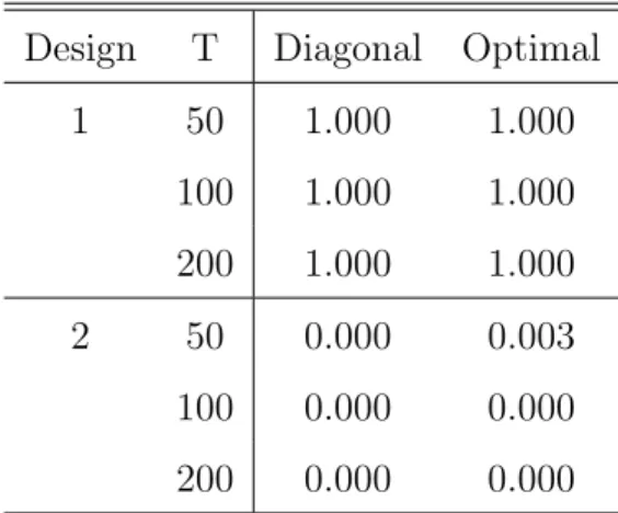
and the corresponding five elements in the covariance matrix of the three observed variables, where we set σ = 1 and κ = 0.5. We consider two cases. In case 1, the two parameters are estimated in model A, while σ is estimated and the value of κ is set to a wrong parameter value, 1, in model B. In other words, model A is correctly 3
specified and model B is incorrectly specified. In case 2, only one parameter (σ) is estimated and the value ofκ is set to the true parameter value in model A, while the two parameters are estimated in model B. Although the two models are both correctly specified in this design, model A is more parsimonious than model B.
Suppose that we employ a classical minimum distance (CMD) estimator and choose the model with a smaller estimation criterion function. Table 1 shows the frequencies of selecting the right model (model A) when one selects a model with a smaller value of the minimized estimation criterion function. The number of Monte Carlo replications is 1,000 and the sample sizes are 50, 100 and 200. The column labeled “Diagonal” indicates the selection probabilities when the diagonal weighting matrix whose diagonal elements are the reciprocals of the bootstrap variances of the sample analogs of the restrictions. The column labeled “Optimal” indicates those when the weighting matrix is the inverse of the bootstrap covariance matrix of the sample analog of the restrictions. This table shows that although this intuitive procedure tends to select the correctly specified models over the incorrectly specified models in designs 1, it is likely to select an overparameterized model if the two models have equal explanatory power as in population as in cases 2. Our proposed QML model selection criteria overcome this issue as formally shown in the next section.
Furthermore, the issue of weak and partial identification is often encountered in macroeconomic applications. In this static model example, suppose f(σ, κ) = [κ+
σ2κ,1+κ2+σ2κ2,−σκ]′and the corresponding three elements of the covariance matrix are used to estimate the model instead of (6). As κ approaches zero, the strength of identification of σ becomes weaker. In addition, the slope of NKPC κ is known to depend on more than one deep parameters which are partially identified.
3
Asymptotic Theory
3.1
Quasi-Marginal Likelihood for Extremum Estimators
We first consider QMLs based on general objective functions and establish the consis-tency of the model selection based on QMLs. Models A and B are parameterized by vectors, α ∈ A and β ∈B, respectively, where A ⊂ ℜpA and B ⊂ ℜpB. Let ˆq
A,T(α)
and ˆqB,T(β) be the objective functions for estimating models A and B, respectively,
that would be minimized in the conventional frequentist estimation method. Here subscript T signifies the fact that both objective functions are constructed using the same data with sample size T. The conventional extremum estimators are given by
ˆ
αT = arg minα∈AqˆA,T(α) and ˆβT = arg minβ∈BqˆB,T(β). Let qA(α) and qB(β) denote
the population analog of ˆqA,T(α) and ˆqB,T(β), and define the (possibly pseudo) true
parameter values of α and β by α0 = arg minα∈AqA(α) and β0 = arg minβ∈BqB(β),
respectively.
In this paper, we say model A is nested in model B if there exist a functionφ:ℜpA →
ℜpB such that q
A(α) = qB(φ(α)), for allα ∈A.4 Rivers and Vuong (2002) generalize
a likelihood ratio test for model comparison originally developed by Vuong (1989) to the case of extremum estimators and show that ˆqA,T(ˆαT)−qˆB,T( ˆβT) =Op(T−1) if the
models are nested and that ˆqA,T(ˆαT)−qˆB,T( ˆβT) =Op(T−
1
2) otherwise. Hnatkovska,
Marmer and Tang (2012) and Smith (1992) show similar results for CMD estimators and GMM estimators, respectively.
Following Chernozhukov and Hong (2003), the quasi-posteriors of models A and B can be defined by
e−TqˆA,T(α)π
A(α)
R
Ae−TqˆA,T(α)πA(α)dα
and e
−TqˆB,T(β)π
B(β)
R
Be−TqˆB,T(β)πB(β)dβ
, (7)
whereπA(α) andπB(β) are the prior probability density functions for the two models.
By treating (7) as the posterior, their LTE (e.g., quasi-posterior mean, median and mode) is obtained via Markov Chain Monte Carlo (MCMC) which may be particularly useful when the objective functions are is not numerically tractable or when extremum estimates are not reasonable.
4
We now define the QMLs for models A and B by
mA =
Z
A
e−TqˆA,T(α)π
A(α)dα andmB =
Z
B
e−TqˆB,T(β)π
B(β)dβ. (8)
We say that the QML model selection criterion is consistent in the following sense:
mA> mB with probability approaching one ifqA(α0)< qB(β0) or ifqA(α0) =qB(β0) and pAs < pBs where pAs and pBs are the numbers of strongly identified parameters in models A and B, respectively. For example, suppose the parameter α in model A corresponds to a subset of the parameterβ in model B so that two models are nested, and a remaining part of parameter β are fixed at their true value. Then, β0 =φ(α0) and qA(α0) =qB(β0) hold and the model with the fixed parameter value is preferable
because it reduces parameter estimation uncertainty. This definition of consistency is common in the literature on selection of parametric models (see Leeb and P¨otscher, 2009; Nishii, 1988; and Inoue and Kilian, 2006 to name a few), and the model selection criteria, such as those in Nishii (1988), Sin and White (1996) and Hong and Preston (2012), are designed to be consistent in this sense. 5 In order that the model selection based on the value ofqA(α0) andpAs relative to the value of qB(β0) and pBs to make sense, every object of model selection needs to be incorporated in criterion functions and parameter vectors. We will be more specific about this issue when we remark on Propositions 1 and 2 in the next two subsections.
It can be shown that the log of the QML is approximated by
ln(mA) = −TqbA,T(αbT)−
pA
2 ln(T) +Op(1), (9) ln(mB) = −TqbB,T(βbT)−
pB
2 ln(T) +Op(1). (10)
Because the leading term diverges at rateT, a correctly specified model will be chosen over an incorrectly specified model. When the model is nested and qA(α0) =qB(β0), a more parsimonious model will be chosen because of the second term. The problem is when the model is not nested and qA(α0) = qB(β0). Because the difference of the dominant terms can have either sign with positive probability and diverges at rate
T1/2, a model will be chosen randomly. When two models that are not nested have equal fit, one may still prefer a more parsimonious model based on Occam’s razor or
5
One could also call a model selection criterion consistent ifmA> mB with probability approaching one
if a selected model is to be used for forecasting (Inoue and Kilian, 2006). For that purpose we propose the followingmodified QML:
ln( ˜mA) = ln(mA) + (T−
√
T)ˆqA,T(ˆαT), (11)
ln( ˜mB) = ln(mB) + (T −
√
T)ˆqB,T( ˆβT). (12)
In the logarithmic form, the modified QML effectively replaces −TqˆA,T(ˆαT) in the
Laplace approximation by −√TqˆA,T(ˆαT) so that T
1
2(qbA,T(αbT)−qbB,T(βbT)) = Op(1)
and the more parsimonious model will be selected in the equal-fit case, and the modi-fied QML model selection criterion remains consistent for both nested and nonnested models.
Let αs and βs denote strongly identified parameters if any, αw and βw weakly
identified parameters, and αp and βp partially identified parameters. pAs and pBs denote the number of the strongly identified parameters, pAw and pBw the number of the weakly identified parameters, andpApandpBpthe number of the partially identified parameters. AsandBsare the spaces of the strongly identified parameters,AwandBw
are those of the weakly identified parameters, andAp andBp are those of the partially
identified parameters. We consider two cases. Some of the parameters may be weakly identified in the first case (α= [α′sα′w]′,pA=pAs+pAw, andA=As×Aw) while some parameters may be partially identified in the second case (α= [α′sα′p]′,pA=pAs+pAp and A=As×Ap). The parameters may be all strongly identified (pA=pAs), weakly identified (pA=pAw) or partially identified (pA=pAp).
Assumption 1
(a) Ais compact inℜpA [B is compact inℜpB].
(b) IfpAs >0,qbA(α) andqA(α) are twice continuously differentiable inαs∈int(As), supα∈A|qbA,T(α)−qA(α)| = op(1), supα∈Ak∇αsqbA,T(α)− ∇αsqA(α)k = op(1) and supα∈Ak∇2αsqbA,T(α)− ∇2αsqA(α)k = op(1) [If pBs > 0, qbB(β) and qB(β) are twice continuously differentiable inβs∈int(Bs), supβ∈B|qbB,T(β)−qB(β)| =
op(1), supβ∈Bk∇βsqbB,T(β)− ∇βsqB(β)k = op(1) and supβ∈Bk∇ 2
βsbqB,T(β)−
∇2βsqB(β)k = op(1)].
Assumption 1(b) requires uniform convergence of ˆqA,T(·), ∇qˆA,T(·) and ∇2qA,T(·) to
qA(·),∇qA(·) and∇2qA(·), respectively, which holds under more primitive assumptions,
such as the compactness of the parameter spaces, pointwise convergence and stochastic equicontinuity (see Theorem 1 of Andrews, 1992).
It is well-known that some parameters of DSGE models may not be strongly identi-fied. See Canova and Sala (2009), for example. It is therefore important to investigate asymptotic properties of our model selection procedure in case some parameters may not be strongly identified. To allow for some weakly identified parameters, we impose the following assumptions:
Assumption 2 (Weak Identification)
(a) qA(α) =qAs(αs) +T −1q
Aw(α) if pAs >0 and qA(αw) =T −1q
Aw(αw) if pAs = 0 where qAw(·) is Op(1) uniformly in α ∈ A. [qB(β) = qBs(βs) +T
−1q
Bw(β) if
pBs >0 andqB(βw) =T −1q
Bw(βw) ifpBs = 0 where qBw(·) is Op(1) uniformly in
β∈B].
(b) If pAs >0, then there exists αs,0∈int(As) such that for every ǫ >0
inf
αs∈As:kαs−αs,0k≥ǫ
qAs(αs) > qAs(αs,0)
[IfpBs >0, then there existsβs,0 ∈int(Bs) such that for everyǫ >0
inf
βs∈Bs:kβs−βs,0k≥ǫ
qBs(βs) > qBs(βs,0)].
(c) IfpAs >0, the Hessian ∇2αsqAs(αs,0) is positive definite [ If pBs >0, the Hessian
∇2βsqBs(βs,0) is positive definite].
Remarks.
1. Assumptions 1 and 2 are high-level assumptions, and sufficient and lower-level assumptions for CMD and GMM estimators are provided in the next two subsections. 2. Typical prior densities are continuous in macroeconomic applications, and Assump-tion 1(c) is likely to be satisfied.
3. Assumption 2(a) postulates that αw is weakly identified while αs is strongly
iden-tified where α = [α′
s α′w]′. Note that we allow for cases in which the parameters are
there is a strongly identified parameter, Assumption 2(b) requires that its true param-eter value αs,0 uniquely minimizes the population estimation criterion function, and Assumption 2(c) requires that the second-order sufficient condition for minimization is satisfied.
Theorem 1 (The Case When Some Parameters May Be Weakly Identified). Suppose that Assumptions 1 and 2 hold.
(a) If qAs(αs,0) < qBs(βs,0), then mA > mB and ˜mA > m˜B with probability ap-proaching one.
(b) (Nested Case) If qAs(αs,0) = qBs(βs,0), pAs < pBs and qbA,T(αbT)−qbB,T(βbT) =
Op(T−1), then mA> mB and ˜mA>m˜B with probability approaching one.
(c) (Nonnested Cases) IfqAs(αs,0) =qBs(βs,0),pAs < pBs andqbA,T(αbT)−qbB,T(βbT) =
Op(T−1/2), then ˜mA>m˜B with probability approaching one.
Remarks.
1. Theorem 1(a) shows that the proposed QML model selection criterion selects the model with a smaller population estimation criterion function with probability ap-proaching one. Theorem 1(b) implies that, if the minimized population criterion func-tions take the same value, our model selection criterion will select the model with a fewer number of strongly identified parameters. In the special case where Model A is correctly specified and is a restricted version of Model B, our criterion will select Model A provided the restriction is imposed on a strongly identified parameter. This is because the QML has a built-in penalty term for parameters that are not necessary for reducing the population criterion function as can be seen in the Laplace approximation of the marginal likelihood. Note that these results hold even when the parameters are all strongly identified.
that case, our model selection criterion will select the better approximating model with probability approaching one.
3. When the models are not nested and qA(αs,0) = qB(βs,0), Theorem 1(c) shows that the marginal likelihood does not necessarily select a more parsimonious model even asymptotically. This is consistent with Hong and Preston’s (2012) result on BIC. Although this may not be a major concern when the models are nonnested, the modified QML selects a parsimonious model even when the nonnested models satisfy qA(αs,0) =qB(βs,0). However, because the leading term in the modified QML diverges at rate √T, the modified QML is less powerful than the unmodified QML if
qA(αs,0)< qB(βs,0). We will investigate this trade-off in Monte Carlo experiments.
Next we consider cases in which some parameters may be partially identified. We say that the parameters are partially identified if A0 = {α0 ∈ A : qA(α0) =
minα∈AqA(α)}consists of more than one points (see Chernozhukov, Hong and Tamer,
2007). Moon and Schorfheide (2012) lists macroeconometric examples in which this type of identification arises. Similarly, we define B0 = {β0 ∈ B : qB(β0) = minβ∈BqB(β)}. In addition to Assumption 1, we impose the following assumptions.
Assumption 3 (Partial Identification)
(a) There existsA0⊂Asuch that, for everyα0∈A0 andǫ >0 infα∈(Ac
0)−ǫqA(α) >
qA(α0), where (Ac0)−ǫ = {α∈A:d(α,A0)≥ǫ}andd(α,A0) = infa∈A0kα−ak[
There existsB0⊂Bsuch that, for everyβ0 ∈B0andǫ >0, infα∈(Ac
0)−ǫqA(α) >
qA(α0), where (Bc0)−ǫ = {β∈B:d(β,B0)≥ǫ}andd(β,B0) = infb∈B0kβ−bk.]
(b) If pAs > 0, the Hessian ∇ 2
αsqA([α ′
s,0, α′p,0]′) is positive definite for some αp,0 ∈ Ap,0. [ If pBs > 0, the Hessian ∇2βsqB([βs,′ 0, βp,′ 0]′) is positive definite for some
βp,0∈Bp,0].
(c) RA
p,0πA(αp|αs,0)dαp > 0 where πA(αp|αs) is the prior density of αp conditional
on αs. [RBp,0πB(βp|βs,0)dβp >0 where πB(βp|αs) is the prior density of βp
con-ditional onβs].
and 1(c), respectively, to sets.
Theorem 2 (The Case When Some Parameters May Be Partially Identified).
(a) Suppose that Assumptions 1 and 3(a) hold. If minα∈AqA(α) < minβ∈BqB(β),
thenmA> mB and ˜mA>m˜B with probability approaching one.
(b) (Nested Case) Suppose that Assumptions 1 and 3 hold. If qAs(αs,0) =qBs(βs,0),
pAs < pBs and qbA,T(αbT)−qbB,T(βbT) = Op(T
−1), then m
A > mB and ˜mA >m˜B
with probability approaching one.
(c) (Nonnested Cases) Suppose that Assumption 3 holds. If qAs(αs,0) = qBs(βs,0),
pAs < pBsandbqA,T(αbT)−qbB,T(βbT) =Op(T
−1/2), then ˜m
A>m˜Bwith probability
approaching one.
Remarks
Theorem 3(a) shows that even in the presence of partially identified parameters, our criteria select a model with a smaller value of the population estimation objective function. This result occurs because it is the value of the objective function, not the parameter value, that matters to model selection.
3.2
Quasi-Marginal Likelihood for CMD Estimators
Since the extremum estimators include some class of important estimators popularly used in practice, it should be useful to describe a set of assumptions specific to each of the estimators. We first consider the CMD estimator, which has been used to estimate the structural parameters in DSGE models by matching the predicted impulse response function (say, DSGE-IRF) and the estimated impulse response function from the VAR models (say, VAR-IRF) in empirical macroeconomics.
Suppose that we compare two DSGE models, models A and B. Models A and B are parameterized by structural parameter vectors,α∈Aandβ∈B, whereA⊂ ℜpA and B ⊂ ℜpB. Let f(α) and g(β), of dimensionk×1, denote the DSGE-IRFs of models A and B, respectively. The IRF matching estimator of Christiano, Eichenbaum and Evans (2005) minimizes the criterion functions
ˆ
qA,T(α) =
1
2(ˆγT −f(α)) ′Wc
ˆ
qB,T(β) = 1
2(ˆγT −g(β)) ′Wc
T(ˆγT −g(β)),
with respect to α ∈ A and β ∈ B , respectively, for models A and B, where ˆγT is a
k×1 vector of VAR-IRFs, andcWT is ak×k positive semidefinite weighting matrix.6
It should be noted that the condition for identifying VAR-IRFs must be satisfied in DSGE models. For example, if short-run restrictions are used to identify VAR-IRFs, the restrictions must be satisfied in the DSGE model. Otherwise IRF matching does not yield a consistent estimator and model selection based on IRF matching may become invalid.
Let
qA(α) =
1
2(γ0−f(α)) ′W(γ
0−f(α)), (13)
qB(β) =
1
2(γ0−g(β)) ′W(γ
0−g(β)), (14)
whereγ0 is a vector of population VAR-IRFs and W is a positive definite matrix. While our model selection depends on the choice of weighting matrices, if one is to calculate standard errors from MCMC draws,WcT needs to be set to the inverse of the
asymptotic covariance matrix of ˆγT, which eliminates the arbitrariness of the choice
of the weighting matrix. When the optimal weighting matrix is not used, the formula in Chernozhukov and Hong (2002) and Kormilitsina and Nekipelov (2016) should be used to calculate standard errors.
For CMD estimators, we make the following assumptions:
Assumption 4.
(a) √T(γbT −γ0) →d N(0k×1,Σ) where Σ is positive definite.
(b) Ais compact inℜpA [B is compact inℜpB].
(c) f(α) = fs(αs) +T−1/2fw(α) if pA >0 and f(α) = T−1/2fw(α) if pA = 0, where
fs:As→ ℜk and fw :A→ ℜk are three times continuously differentiable in the
interior ofA. The Jacobian matrix offs,Fs(αs) =∂fs(αs)/∂α′s, has rankpAs at
αs=αs,0 [g:B→ ℜk is three times continuously differentiable in the interior of B, and its Jacobian matrixGs(βs) =∂g(βs)/∂βs′ has rank pBs atβs=βs,0]. 6
(d) cWT is positive semidefinite with probability one and converges in probability to
a positive definite matrixW.
(e) IfpAs >0, there is a uniqueαs,0∈int(As) such thatαs,0 = argminαs∈Asfs(αs) ′W f
s(αs).
If pAs = 0, f(α) = T −1/2f
w(αw) [If pBs > 0, g(β) = gs(βs) +T −1/2g
w(β), and
there is a uniqueβs,0 ∈int(Bs) such thatβs,0 = argminβs∈Bsgs(βs) ′W g
s(βs). If
pBs = 0,g(β) =T −1/2g
w(βw).
(f) IfpAs >0,
Fs(αs,0)′W Fs(αs,0)−[(γ−fs(αs,0))′W ⊗IpAs,0]∂vec(Fs(αs,0)
′)
∂α′
s,0 is positive definite [ IfpBs >0,
Gs(βs,0)′W Gs(βs,0)−[(γ−gs(βs,0))′W ⊗IpBs]
∂vec(Gs(βs,0)′)
∂β′
s
is positive definite].
(g) There is A0 = {α0} ×Ap,0 ⊂ A such that, for any α ∈ A0, (γ−f(α))′W(γ−
f(α)) = minα˜∈A(γ −f(˜α))′W(γ −f(˜α)) < (γ −f(¯α))′W(γ − f(¯α)) for any ¯
α ∈ A∩ Ac0 [There is B0 = {β0} × Bp,0 ⊂ B such that, for any β ∈ B0, (γ−g(β))′W(γ−g(β)) = min
˜
β∈B(γ−g( ˜β))′W(γ−g( ˜β))<(γ−g( ¯β))′W(γ−g( ¯β)) for any ¯β ∈B∩Bc0].
(h) IfpAs >0, there is αp,0 ∈Ap,0 such that
Fs(α)′W Fs(α)−[(γ−f(α))′W ⊗IpAs]
∂vec(Fs(α)′)
∂α′
s
,
is positive definite atα= [α′s,0 α′p,0]′ [ IfpBs >0, there isβp,0 ∈Bp,0 such that
Gs(β)′W Gs(β)−[(γ−g(β))′W ⊗IpBs]∂vec(Gs(β)
′)
∂β′
s
,
is positive definite atβ= [βs,′ 0βp,′ 0]′].
Remarks.
2. Assumption 4(e) follows Guerron-Quintana, Inoue and Kilian’s (2013) definition of weak identification in the minimum distance framework.
The model selection based on the QML computed from quasi-Bayesian CMD Esti-mators is justified by the following proposition.
Proposition 1.
(a) Under Assumptions 4(a)–(f), Assumptions 1 and 2 hold.
(b) Under Assumptions 4(a)–(d), (g) and (h), Assumptions 1 and 3 hold.
Remark. In our framework, the VAR-IRF,bγT, is common across different DSGE models
and our proposed QML is designed to select a DSGE model. When it is used to select VAR-IRFs given a DSGE model, the QML will select all the valid impulse responses, that is, all the VAR-IRFs that equal the corresponding DSGE-IRFs (see Hall, Inoue, Nason and Rossi, 2012, on this issue). When it is used to select the number of lags in the VAR model given an IRF and a DSGE model, the QML will select enough many lags so that the implied VAR-IRF equals the DSGE-IRF provided that the population VAR-IRF equals the corresponding DSGE-IRF for sufficiently many lags. However, it will not necessarily choose the smallest lag for which the implied VAR-IRF equals the DSGE-IRF with probability approaching one. This is because the criterion function is not used in the VAR parameter estimation. If the goal is to select the number of lags, the criterion function and the parameter vector need to be modified.
3.3
Quasi-Marginal Likelihood for GMM Estimators
Another important class of the estimator we consider is the GMM estimator. For GMM estimators, the criterion functions of models A and B are respectively given by
ˆ
qA,T(α) =
1 2fT(α)
′cW
A,T fT(α),
ˆ
qB,T(β) =
1 2gT(β)
′cW
B,TgT(β),
wherefT(α) = (1/T)PtT=1f(xt, α), gT(β) = (1/T)PTt=1g(xt, β) and WcA,T and WcB,T
Let
qA(α) =
1
2E[f(xt, α)] ′W
AE[f(xt, α)], (15)
qB(β) =
1
2E[g(xt, β)] ′W
BE[g(xt, β)], (16)
whereWAand WB are positive definite matrices.
For the GMM estimation, we impose the following assumptions:
Assumption 5.
(a) supα∈AkT−1PT
t=1{f(xt, α)−E[f(xt, α)]}k = Op(T−1/2), supα∈AkT−1 PT
t=1{(∂/∂α′)f(xt, α)−
E[(∂/∂α′)f(xt, α)]}k = op(1), and supα∈AkT−1 PT
t=1{(∂/∂α′)vec((∂/∂α′)f(xt, α)−
E[(∂/∂α′)vec((∂/∂α′)f(x
t, α))]}k = op(1) [supβ∈BkT−1 PT
t=1{g(xt, β)−E[g(xt, β)]}k =
Op(T−1/2), supβ∈BkT−1 PT
t=1{(∂/∂β′)g(xt, β)−E[(∂/∂β′)g(xt, β)]}k = op(1),
and supβ∈BkT−1PT
t=1{(∂/∂β′)vec((∂/∂β′)g(xt, β)−E[(∂/∂β′)vec((∂/∂β′)g(xt, β))]}k =
op(1)].
(b) Ais compact inℜpA [B is compact inℜpB].
(c) f :X ×A→ ℜk is three times continuously differentiable in α in the interior of A, and Fs(αs) = ∂E[f(xt, αs)/∂αs′] has rankpAs atαs =αs,0 [g :X ×B → ℜℓ is three times continuously differentiable inβ in the interior ofB, and Gs(βs) =
E[∂g(xt, βs)/∂βs′] has rank pBs atβs=βs,0].
(d) cWA,T is positive semidefinite with probability one and converges in probability
to a positive definite matrixWA [cWB,T is positive semidefinite with probability
one and converges in probability to a positive definite matrixWB].
(e) If pAs > 0, E[f(xt, α)] = fs(αs) +T −1/2f
w(α), and there is a unique αs,0 ∈ int(As) such thatαs,0 = argminαs∈Asfs(αs)
′W
Afs(αs). IfpAs = 0, E[f(xt, α)] =
T−1/2fw(αw) [If pBs > 0, E[g(xt, β)] = gs(βs) + T −1/2g
w(β), and there is a
uniqueβs,0 ∈int(Bs) such that βs,0 ∈argminβs∈Bsgs(βs) ′W
Bgs(βs). If pBs = 0,
E[g(xt, β)] =T−1/2gw(βw)].
(f) IfpAs >0,
Fs(αs,0)′WAFs(αs,0) + [E(fs(xt, αs,0))′WA⊗IpAs]
∂vec(Fs(αs,0)′)
∂α′
is positive definite [ IfpBs >0,
Gs(βs,0)′WBGs(βs,0) + [(γ−gs(βs,0))′WB⊗IpBs]
∂vec(Gs(βs,0)′)
∂β′
s
is positive definite].
(g) There isA0 ={α0}×Ap,0⊂Asuch that, for anyα∈A0,E[f(xt, α)]′WAE[f(xt, α)] =
min˜α∈AE[f(xt,α˜)]′WAE[f(xt,α˜)] < E[f(xt,α¯)]′WAE[f(xt,α¯)] for any ¯α ∈ A∩
Ac0[There isB0={β0}×Bp,0 ⊂Bsuch that, for anyβ ∈B0,E[g(xt, β)]′WBE[g(xt, β)] =
minβ˜∈BE[g(xt,β˜)]′WBE[g(xt,β˜)] < E[g(xt,β¯)]′WBE[g(xt,β¯)] for any ¯β ∈ B∩
Bc0].
(h) IfpAs >0, there is αp,0 ∈Ap,0 such that
Fs(α)′WAFs(α) + [E(f(xt, α))′WA⊗IpAs]
∂vec(Fs(α)′)
∂α′
s
is positive definite atα= [α′
s,0 α′p,0]′ [ IfpBs >0, there isβp,0 ∈Bp,0 such that
Gs(β)′WBGs(β) + [E(g(xt, β))′WB⊗IpBs]
∂vec(Gs(β)′)
∂β′
s
is positive definite atβ= [βs,′ 0βp,′ 0]′.
The model selection based on the QML computed from quasi-Bayesian GMM Es-timators is justified by the following proposition.
Proposition 2.
(a) Under Assumptions 5(a)–(f), Assumptions 1 and 2 hold.
(b) Under Assumptions 5(a)–(d), (g) and (h), Assumptions 1 and 3 hold.
4
Discussions
Although our method is applicable to more general problems, one main motivation for our proposed QML model selection is IRF matching. IRF matching is a limited-information approach and is an alternative to full-limited-information likelihood based ap-proaches, such as MLE and Bayesian approaches. Estimators based on the full-information likelihood are more efficient when the likelihood function is correctly spec-ified, while IRF matching estimators may be more robust to potential misspecification that does not affect the IRF, such as misspecification of distributional forms. In addi-tion to this usual tradeoff between efficiency and robustness, we discuss very particular features IRF matching estimators have.
(a) Bayesian and frequentist inferential frameworks for IRF matching: The use of priors not only alleviates such numerical challenges inherent in IRF matching but also gives a limited-information Bayesian interpretation to IRF matching (Kim, 2002; Zellner, 1998). Because the QML is a functions of data, which model is selected is also a function of the data. Because the quasi-posterior distribution is conditional on the data and the result of model selection is a function of the conditioning set, the posterior distribution remains the same. Therefore, there is no issue of post model selection inference in the limited-information Bayesian inferential framework. See Dawid (1994) in the full-information Bayesian inferential framework.
It is often useful to have a frequentist interpretation of Bayesian estimators, espe-cially if the practitioner is not strictly a Bayesian. Chernozhukov and Hong (2002) provides consistency and asymptotic normality of LTE that includes IRF matching estimators as a special case. Our paper shows the consistency of the QML model se-lection criterion in a frequentist inferential framework. When we interpret inference based on the model selected by our model selection criterion in a frequentist inferential framework, it is likely to suffer from the problem with post model selection inference (Leeb and P¨otscher, 2005, 2009), which is typical in model selection.
in a DSGE model and the number of observed variables are the same. Fern´ andez-Villaverde, Rubio-Ram´ırez, Sargent and Watson (2007) find a sufficient condition for the two sets of structural IRF to match. One of their conditions is that matrixD in the measurement equation is square and is nonsingular. Even when this condition is not satisfied (e.g., no measurement error), there are cases in which the two structural IRFs coincide. For example, consider
xt+1 = Axt+But+1, (17)
yt+1 = Cxt, (18)
where xt is a n×1 vector of state variables, yt and ut are k×1 vectors of observed
variables and economic shocks, respectively, andutis Gaussian white noise vector with
zero mean and covariance matrix Ik. Provided the eigenvalues of A are all less than
unity in modulus,yt has an M A(∞) representation:
yt = C(I−AL)−1But = CBut+CABut−1+CA2But−2+· · · (19)
and it is invertible. Thus, the structural IRFs,CB,CAB,CA2B, ..., can be obtained from a VAR(∞) process together with the short-run restriction that the impact matrix is given by CB. In practice, the VAR(∞) process is approximated by a finite-order VAR(p) model wherepis obtained by AIC, for example. In the IRF matching literature it is quite common to build a DSGE model in such a way thatCB is lower triangular so that the recursive identification condition can be used to identify structural IRFs from a VAR model. Many DSGE models do not satisfy typical short-run conditions for identifying structural impulse responses. There are at least two approaches. First, one can match IRFs without matching the impact period matrix. Let Aj denote the jth
step ahead structural impulse response matrix implied by a DSGE model withA0being the impact matrix. Let Bj denote the jth step ahead reduced-form impulse response
matrix obtained from a VAR model. Then we have Σ = A0A′0andBjA0 = Aj, which
in turn can be written asg(γ, θ) = 0, whereγ is a vector that consists of the elements of Bj’s and the distinct elements of Σ and θ is a vector of DSGE parameters. In the
second approach, one can match moments (e.g., Andreasen, Fern´andez-Villaverde and Rubio-Ram´ırez, 2016; Kormilitsina and Nekipelov, 2016).
Inoue, Nason and Rossi (2012) show that the performance of IRF matching estimators deteriorates as the number of IRFs increases. Guerron-Quintana, Inoue and Kilian (2016) show that, when the number of impulse responses is greater than the number of VAR parameters, IRF matching estimators have nonstandard asymptotic distributions because the delta method fails. We conjecture that asymptotic properties of the QML model selection criterion may be affected because the bootstrap covariance matrix estimator is asymptotically singular.
In general, we recommend to select the order of VAR models by information criteria, such as AIC, as done in section 6 because the true VAR representation is likely to be of infinite order. We then suggest to choose the maximum horizon so that the number of impulse response does not exceed the number of VAR parameters to avoid the above issue.
function by any number without changing its optimum. Using the optimal weighting matrix eliminates such arbitrariness in the CMD and GMM frameworks.
(e) The use of modified QMLs: There may be some cases the modified QMLs are recommended over the (unmodified) QMLs in model selection because of the possible inconsistency. One possibility is the case of point mass mixture priors which include a mass at a point mixed with a continuous distribution. For example, suppose two alternative models of nominal exchange rates,St, as
Model A (IMA(1) model) α=θ: ∆St=εt+θεt−1.
Model B (AR(2) model)β = (φ1, φ2): St=φ1St−1+φ2St−2+εt.
The two models are non-nested but are equivalent under the random walk speci-fication, namely, if θ = 0 in model A and (φ1, φ2) = (1,0) in model B. Because the random walk model is known to be supported by many previous empirical studies as a preferred model for the nominal exchange rate, it make sense to employ point mass priors at θ= 0 in model A and (φ1, φ2) = (1,0) in model B. If the true model is the random walk model, the (unmodified) QML will select model B with positive probabil-ity. The modified QML will select model A over model B with probability approaching one because the former is more parsimonious, however.
5
Guide for practitioners
We describe how to implement our procedure in this section. First, we specify a quasi-likelihood function and estimate the model by the random-walk Metropolis Hasting algorithm. As discussed in the previous section, we recommend to use the optimal weighting matrix, the inverse of the covariance matrix for bootstrap IRF estimates although we also consider the diagonal weighting matrix in the Monte Carlo experi-ments in section 6. As suggested in An and Schorfheide (2007), we set the proposal distribution toN(α(j−1), cHˆ−1) whereα(0)= ˆα,c= 0.3 forj = 1,c= 1 forj >1 and
ˆ
H is the Hessian of the log-quasi-posterior evaluated at the quasi-posterior mode. The drawα from N(α(j−1), c[∇2qˆA,T(ˆα)]−1) is accepted with probability
min 1, e
−TˆqA,T(α)π
A(α)
e−TqˆA,T(α(j−1))
πA(α(j−1))
!
In section 6, we use 50,000 draws.
Second, we compute the QML using the last half of the draws. We consider four methods for computing the QML: Laplace approximations, modified harmonic estima-tors of Geweke (1998) and Sims, Waggoner, and Zha (2008) and the estimator of Chib and Jeliazkov (2001). For the Laplace approximation, we evaluate the QML by
e−T qA( ˆα)
T
2π
k−pA
2
πA( ˆα)|cWT|
1
2|∇2qˆA,T(ˆα)|−12, (21)
at the quasi-posterior mode, ˆα (here subscriptT is omitted for notational simplicity). In our Monte Carlo experiment, we use 20 randomly chosen starting values for a nu-merical optimization routine to obtain the posterior mode. We use 1,000 bootstrap replications to obtain the bootstrap covariance matrix of IRF estimators in the Monte Carlo experiments.
In the modified harmonic mean method, the QML is computed as the reciprocal of
E
w(α)
exp(−TqˆT(α))πA(α)
, (22)
which is evaluated using MCMC draws, given a weighting functionw(α). We consider two alternative choice of weighting functions which have been proposed in the literature. The first choice is suggested by Geweke (1999), who sets w(α) to be the truncated normal density
w(α) = exp[−(α−α˜) ′V˜−1
α (α−α˜)/2]
(2π)pA/2|V˜
α|1/2
1{(α−α˜)′V˜α−1(α−α˜)< χ2pA,τ}
τ ,
where ˜α is the quasi-posterior mean, ˜Vα is the quasi-posterior covariance matrix, 1{·}
is an indicator function, χ2
pA,τ is the 100τth percentile of the chi-square distribution withpA degrees of freedom, and τ ∈(0,1) is a constant. The second choice is the one
proposed by Sims, Waggoner, and Zha (2008). They point out that Geweke’s (1999) method may not work well when the posterior distribution is non-elliptical, and suggest an weighting function given by
w(α) = Γ(pA/2) 2πpA/2|Vˆα|1/2
f(r)
rpA−1
1{−Tqˆ(α) + lnπA(α)> L1−q}
¯
τ ,
where ˆVα is the second moment matrix centered around the quasi-posterior mode ˜α,
percentile of the log quasi-posterior distribution, q ∈ (0,1) is a constant, and τ is the quasi-posterior mean of 1{−Tqˆ(α) + lnπA(α) > L1−q}1{c1 < r < c90/(0.9)1/v}. Following Herbst and Schorfheide (2015), we considerτ = 0.5 and 0.9 in the estimator of Geweke (1999) and q = 0.5 and 0.9 in the estimator of Sims, Waggoner, and Zha (2008). In the Monte Carlo and empirical application sections, we only report the results forτ = 0.9 andq= 0.9 to save space.7
For the estimator of Chib and Jeliazkov (2001), the log of the QML is evaluated by
lnπA(˜α)−TqˆA,T(˜α)−ln ˆpA(˜α) (23)
where
ˆ
pA(α) =
(1/J)PJj=1r(α(j),α˜)φα,c˜ 2Σ˜(α(j))
(1/K)PKk=1r(˜α, α(k)) , (24)
φα,c˜ 2Σ˜(·) is the pdf ofN(˜α, c2Σ) and˜ r(˜α, α(k)) is the acceptance probability of moving ˜
α to α(k) in the Metropolis Hasting algorithm. The numerator of (24) is evaluated using the last 50% of MCMC draws and the denominator is evaluated using α(k) from
N( ˜α, c2Σ). In our Monte Carlo experiment,˜ K is set to 25,000 so that K = J. c2Σ˜ is either set to the one used in the proposal density or estimated from the posterior draws.
The modified QML (11) requires minimizing the estimation criterion function, which may defeat the purpose of using the quasi-Bayesian approach. Instead we ap-proximate it by averaging the values of the log of the quasi-posterior density over quasi-posterior draws:
E[ln(πA(α))−TqbA,T(α)], (25)
where the expectation is with respect to the quasi-posterior draws. This is computa-tionally tractable because it can be calculated from MCMC draws. Because the quasi-posterior distribution will concentrate around αb asymptotically, and the log prior is
O(1) and does not affect the divergence rate of the modified QML, the resulting mod-ified QML model selection criterion remains consistent as analyzed in the previous section. Our Monte Carlo results show that this approximation works well.
7
6
Monte Carlo Experiments
We investigate the small-sample properties of the QML using the small-scale DSGE model considered in Guerron-Quintana, Inoue and Kilian (2016) that consists of
yt = E(yt+1|It−1)−σ[E(Rt|It−1)−E(πt+1|It−1)−zt], (26)
πt = δE(πt+1|It−1) +κyt, (27)
Rt = ρrRt−1+ (1−ρr)(φππt+φyyt) +ξt, (28)
where yt, πt and Rt denote the output gap, inflation rate, and nominal interest rate,
respectively, andItdenotes the information set at timet. The technology and monetary
policy shocks follow
zt = ρzzt−1+σzεzt, (29)
ξt = σrεrt, (30)
whereεzt andεrt are independent iid standard normal random variables. Note that the timing of the information is nonstandard, e.g.,E(πt+1|It−1) instead ofE(πt+1|It) in the
NKPC. The idea behind these information restrictions is to capture that the economy reacts slowly to a monetary policy shock while it reacts contemporaneously to tech-nology shocks. Specifically, inflation does not contemporaneously reacts to monetary policy shocks but it does to technology shocks in this model. We impose such recursive short-run restrictions to identify VAR-IRFs. In the data generating process, we set
κ = 0.025, σ = 1, δ = 0.99, φπ = 1.5, φy = 0.125, ρr = 0.75, ρz = 0.90, σz = 0.30,
σr= 0.20 as in Guerron-Quintana, Inoue and Kilian (2016).
We consider four cases. In cases 1 and 3, κ,σ−1 and ρr are estimated in model A,
andκ andρr are estimated in model B withσ−1= 3. The other parameters are set to
the true parameter values. In cases 2 and 4,σ−1 andρrare estimated in model A with
κset to its true parameter value andκ,σ−1 andρr are estimated in model B. In other
words, model B is misspecified in cases 1 and 3. and model A is more parsimonious than model B in cases 2 and 4.
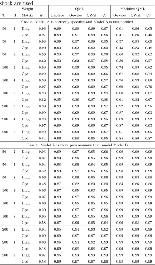
shock contemporaneously, which is satisfied in the above model. In cases 1 and 2, all the structural impulse responses up to horizon H are used in LTE. In cases 3 and 4, only the structural impulse responses to the technology shock (up to horizon
H) are used. We use the AIC to select the VAR lag order where p is selected from
{H, H + 1, ...,[5(T /ln(T))0.25]} where [x] is the integer part of x. We set the lower bound onptoH. Whenpis smaller thanH, the asymptotic distribution of VAR-IRFs is singular and our theoretical results do not hold. See Guerron-Quintana, Inoue and Kilian (2016) on inference on VAR-IRFs in such cases.
We considerT = 50,100,200 andH = 2,4,8. The number of Monte Carlo simula-tions is set to 1,000, the number of random-walk Metropolis-Hasting draws is 50,000, the number of bootstrap draws for computing the weighting matrix is 1,000.
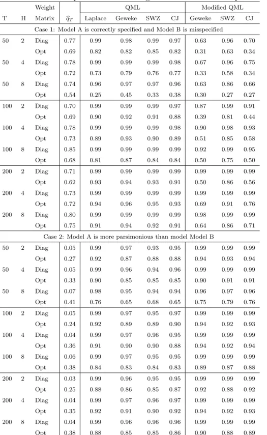
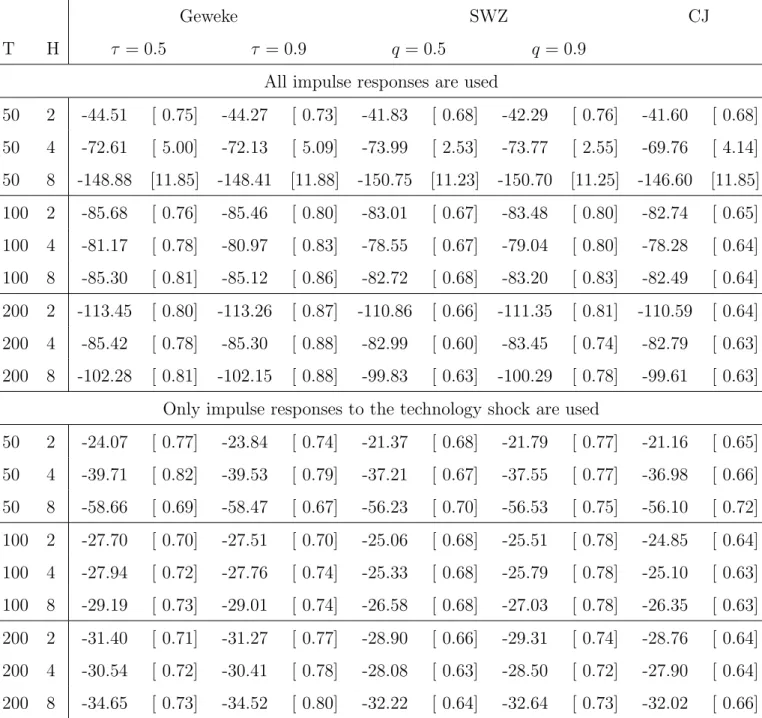
Tables 2 and 3 report the probabilities of selecting model A in cases 1 and 2 and those in cases 3 and 4, respectively. The lower parts of Tables 2 and 3 show that the method of selecting a model based on the value of the estimation criterion function performs poorly when two models are both correctly specified and one model is more parsimonious than the other. The tables show that the probabilities of the QML’s selecting the right model tend to increase as the sample size grows. As conjectured in section 3, the QML performs better than the modified QML when one model is correctly specified and the other is misspecified, and the modified QML outperforms the QML when both are correctly specified and one model is more parsimonious than the other. Using a fewer IRFs, that is, using the IRFs to the technology shock only, improves the performance of the QML. These tables show that the different methods for computing the QML do not produce a substantial or systematic difference in the performance in large samples. The diagonal weighting matrix provides better performance than the optimal weighting matrix but the difference becomes smaller as the sample size grows.8 To shed light on the accuracy of QML estimates further, we report the means and standard deviations of 100 QML estimates from a realization of data in Table 4. Except when many impulse responses are used when the sample size is small (the third row in the table), the standard deviations appear reasonably small. Furthermore, the differences across the methods are small.
8
7
Empirical Applications
7.1
New Keynesian Phillips Curve: GMM Estimation
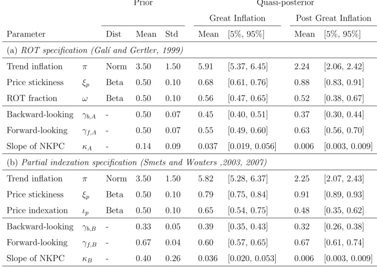
In this section, we apply our procedure to choose between alternative specifications of the structural Phillips curve under nonzero trend inflation when the models are estimated using quasi-Bayesian GMM. Let ˆπt=πt−πbe the log-deviation of aggregate
inflation πt from the trend inflation π, and ˆulct = ulct−ulc be the log-deviation of
unit labor costulct from its steady-stateulc.
In Gal´ı and Gertler (1999), the hybrid New Keynesian Phillips Curve (hereafter NKPC) is derived from a Calvo (1983) type staggered price setting model with firms set prices using indexation to trend inflationπ with probabilityξp (see also Yun, 1996).
For the remaining 1−ξp fraction of the firms, 1−ωfraction of firms set prices optimally
but the remainingωfraction are rule-of-thumb (ROT) price setters who set their prices equal to the average price set in the most recent round of price adjustments with a correction based on the lagged inflation rate. Under these conditions, a hybrid NKPC can be derived as
ˆ
πt=γbπˆt−1+γfEtπˆt+1+κulcˆ t (31)
with its coefficients given by
γb =
ω
ξp+ω[1−ξp(1−δ)]
, γf =
δξp
ξp+ω[1−ξp(1−δ)]
, κ= (1−ξp)(1−δξp)(1−ω)
ξp+ω[1−ξp(1−δ)]
,
whereδ ∈(0,1) is a discounted factor.
In Smets and Wouters (2003, 2007), a partial indexation specification is used instead of the ROT specification of Gal´ı and Gertler (1999). In their specification, firms set prices at an optimal level with probability 1−ξp. For the remainingξp fraction of the
firms, prices are determined as a weighted sum of lagged inflation and trend inflation (or steady state inflation) with an weight ιp on the lagged inflation. Under these
conditions, an alternative hybrid NKPC can be derived as (31) with coefficients given by
γb =
ιp
1 +ιpδ
, γf =
δ
1 +ιpδ
, κ= (1−ξp)(1−δξp)
ξp(1 +ιpδ)
,
whereιp∈[0,1] is the degree of partial indexation to lagged inflation. Note that when
hybrid NKPCs become the baseline NKPC with only forward looking firms (γb = 0
and γf =δ).
In the previous empirical literature, the classical GMM has often been employed to estimate the hybrid NKPC. In our quasi-Bayesian GMM estimation, we utilize the or-thogonality condition of expectation error to past information, as well as the definition of ˆπt = πt−π, and estimate structural parameters α = [ξp, ω, π]′ for the first model
and β = [ξp, ιp, π]′ for the second model. In particular, for the first model, the
objec-tive function is ˆqA,T(α) = (1/2)fT(α)′WcA,T fT(α) wherefT(α) = (1/T)PTt=1f(xt, α),
f(xt, α) = [z′tut,πˆt]′,
ut= ˆπt−γbπˆt−1−γfπˆt+1−κulcˆ t
and zt is a vector of instruments. The objective function for the second model can be
similarly defined. Optimal weighting matrix ˆW is computed from the HAC estimator with the Bartlett kernel and Andrews’ (1991) automatic bandwidth.
For the estimation, we use US quarterly data of the inflation rate based on the GDP implicit price deflator forπtand the labor income share in the non-farm business
sector forulct. As for the choice of instrumentszt, we follow Gal´ı and Gertler (1999):
four lags of inflation, labor income share, long-short interest rate spread, output gap, wage inflation, and commodity price inflation. We use the same set of instruments so that the number of moment conditions is the same for the two NKPCs. For the sample periods, we consider the Great Inflation period (from 1966:Q1 to 1982:Q3) and Post-Great Inflation period (from 1982:Q4 to 2016:Q4). δ is fixed at 0.99.
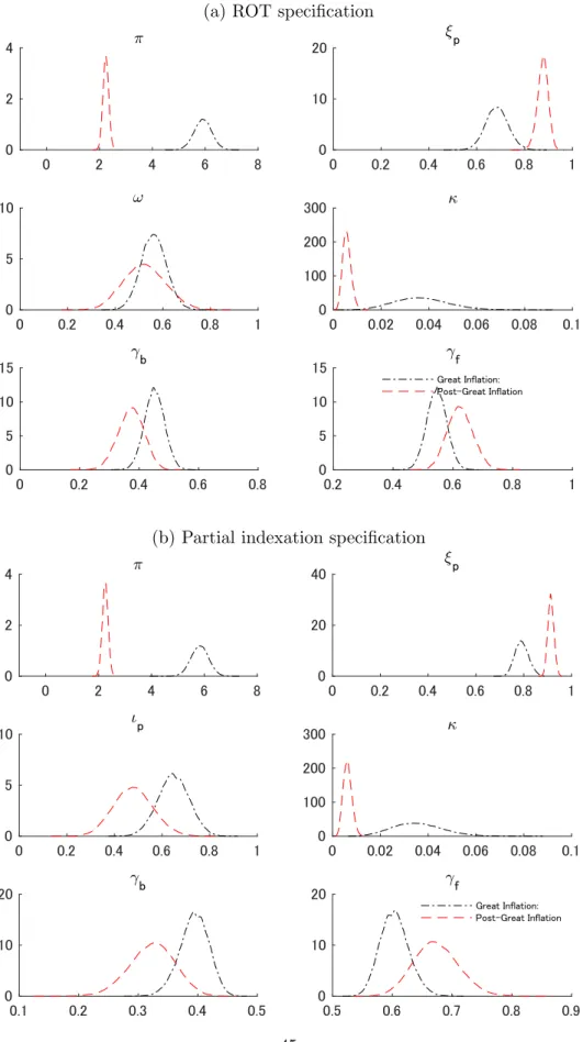
The list of the structural parameters in our analysis, quasi-Bayesian estimates and prior distributions are reported in Table 5 and the posterior distributions are shown in Figure 1 for both ROT specification and partial indexation specification. The prior and posterior means tend to differ which may suggest that the parameters are strongly identified in these models. The trend inflation rate became substantially lower after the Great Inflation period, as expected. The slope of the Phillips curve (κ) got flattened in the post Great Inflation period compared to the Great Inflation period mainly due to the increased degree of price stickiness (ξp). The figure also shows that the slope of the
Phillips curve became more spread. However, in general, both estimates of structural and reduced form parameters differs between two specification. 9
9
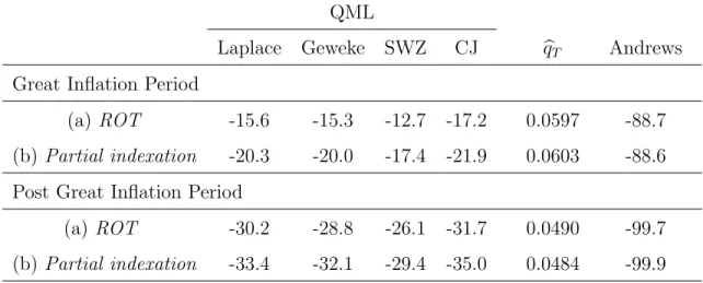
Table 6 reports the QMLs for the two specifications, along with the value of the estimation criterion function and Andrews’(1999) criterion. The results based on com-paring QMLs suggest that the ROT specification of Gal´ı and Gertler (1999) outper-forms the partial indexation specification of Smets and Wouters (2003, 2007) for both sample periods we consider. In particular, according to Jeffreys’(1961) terminology, the former model is decisively better than the latter model.10 For the value of the estimation criterion function and Andrews’(1999) criterion, the model with a smaller value should be selected. When these alternative methods are employed, the ROT specification are selected for the first subsample as in the case of QMLs, but conflict-ing results are obtained for the second subsample. However, since our Monte Carlo results suggest that QMLs are more accurate than the value of the estimation criterion function for selecting correctly specified models in moderate sample sizes, the ROT specification is likely to be the better-fitting specification in the second subsample.
7.2
The Medium-Scale DSGE Model: IRF Matching
Es-timation
As a second empirical application of our procedure, we consider quasi-Bayesian IRF matching estimation of the medium-scale DSGE Model. For the purpose of evaluating the relative importance of various frictions in the model estimated by the standard Bayesian method, Smets and Wouters (2007) utilize the marginal likelihood. Their question is whether all the frictions introduced in the canonical DSGE model are really necessary in order to describe the dynamics of observed aggregate data. To answer this question, they compare marginal likelihoods of estimated models when each of the frictions was drastically reduced one at time. Among the sources of nominal frictions, they claim that both price and wage stickiness are equally important while indexation is relatively unimportant in both goods and labor markets. Regarding the real frictions,
of parameters are different. For example, the ratio of the forward-looking parameter and backward-looking parameter (γf/γb) for the ROT specification depends on three parameters (ξp, ω, δ) while the ratio for the
the partial indexation specification depends only on two parameters (ιp, δ). Such a tighter restriction for the
latter model can make the difference in the empirical performance of two models. 10
they claim that the investment adjustment costs are most important. They also find that, in the presence of wage stickiness, the introduction of variable capacity utilization is less important.
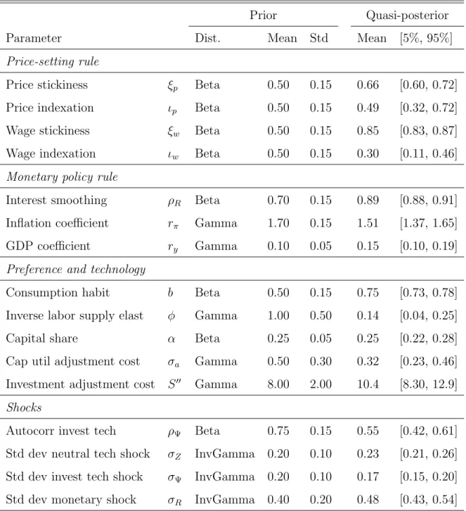
Here, we conduct a similar exercise using QMLs based on the standard DSGE model estimated by Christiano, Trabandt and Walentin (2011). Based on an estimated VAR(2) model of 14 variables using the US quarterly data from 1951Q1 to 2008Q4, they employ short-run and long-run identifying restrictions to compute IRF to (i) a monetary policy shock, (ii) a neutral technology shock and (iii) an investment-specific technology shock. The model is then estimated by matching the first 15 responses of selected 9 variables to 3 shocks, less 8 zero contemporaneous responses to the monetary policy shock (so that the total number of responses to match is 397). Since our purpose is to evaluate the relative contribution of various frictions, we estimate some additional parameters, such as the wage stickiness parameter ξw, wage indexation parameter
ιw and price indexation parameter ιp, which are fixed in the analysis of Christiano,
Trabandt and Walentin (2011).11 The list of estimated structural parameters in our analysis, quasi-Bayesian estimates and the prior distribution, are reported in Table 7. This estimated model serves as the baseline model when we compare with other models using QMLs.
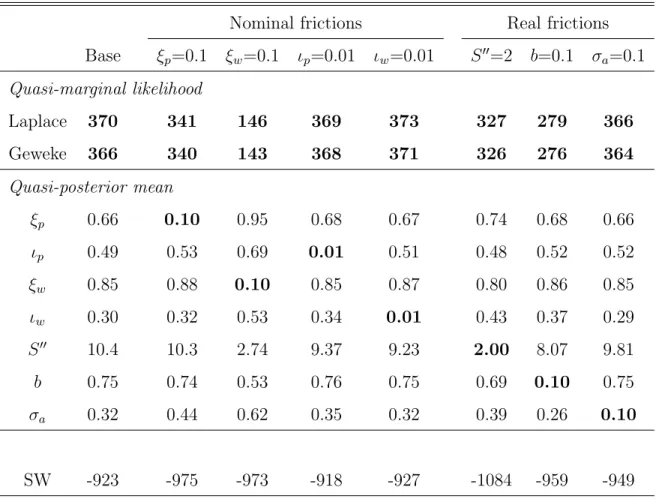
Following Smets and Wouters (2007), the sources of frictions of the baseline model are divided into two groups. First, nominal frictions are sticky prices, sticky wages, price indexation and wage indexation. Second, real frictions are investment adjustment costs, habit formation, and capital utilization. We estimate additional submodels, which reduces the degree of each of the seven frictions. The computed QMLs for 8 models, including the baseline model, are reported in Table 8. For the reference, also included in the table are the original marginal likelihoods obtained by Smets and Wouters (2007) based on the different estimation method applied to the different data set. Let us first consider the role of nominal frictions. According to Jeffreys’(1961) terminology, QMLs are decisively reduced when the degree of nominal price and wage stickiness (ξp andξw) is set at 0.10. In contrast, even if the price and wage indexation
parameters (ιp and ιw) are set at a very small value of 0.01, the values of QMLs are
quite similar to that of the baseline model. Thus, we can conclude that Calvo-type 11
frictions in price and wage settings are empirically more important than the price and wage indexation to past inflation. Let us now turn to the role of real frictions. The remaining three columns show the results when each of investment adjustment cost parameter (S′′), consumption habit parameter (b) and capital utilization cost parameter (σa) is set at some small values. The results show that restricting habit
formation in consumption significantly reduces the QML compared to other two real frictions, suggesting the relatively important role of the consumption habit. Overall, our results seem to support the empirical evidence obtained by Smets and Wouters (2007), despite the fact that our analysis is based on a very different model selection criterion.
8
Concluding Remarks
In this paper we establish the consistency of the model selection criterion based on the QML obtained from Laplace-type estimators. We consider cases in which parameters are strongly identified and are weakly identified. Our Monte Carlo results confirmed our consistency results. Our proposed procedure is also applied to select an appropriate specification in New Keynesian macroeconomic models using US data.
References
An, Sungbae, and Frank Schorfheide (2007), “Bayesian Analysis of DSGE Mod-els,”Econometric Reviews,26, 113–172.
Andreasen, Martin M., Jes´us Fern´andez-Villaverde and Juan Rubio-Ram´ırez (2016), “The Pruned State-Space System for Non-Linear DSGE Models: Theory and Em-pirical Applications,” Working Paper.
Andrews, Donald W.K., (1991), “Heteroskedasticity and Autocorrelation Consis-tent Covariance Matrix Estimation,”Econometrica,59 (3), 817–858.
Andrews, Donald W.K., (1992), “Generic Uniform Convergence,” Econometric
Theory,8, 241–257.
Andrews, Donald W.K., (1999), “Consistent Moment Selection Procedures for Generalized Method of Moments Estimation,”Econometrica, 67, 543–564.
Calvo, Guillermo A. (1983), “Staggered Prices in a Utility-Maximizing Frame-work,”Journal of Monetary Economics, 12 (3), 383–398.
Canova, Fabio, and Luca Sala (2009), “Back to Square One: Identification Issues in DSGE Models,”Journal of Monetary Economics, 56, 431–449.
Chernozhukov, Victor, and Han Hong (2003), “An MCMC Approach to Classical Estimation,”Journal of Econometrics,293–346.
Chernozhukov, Victor, Han Hong and Elie Tamer (2007), “Estimation and Con-fidence Regions for Parameter Sets in Econometric Models,” Econometrica, 75, 1243–1284.
Chib, Siddhartha, and Ivan Jeliazkov (2001), “Marginal Likelihood from the Metropolis-Hastings Output,” Journal of the American Statistical Association,
96, 270–281.
Christiano, Lawrence J., Martin S. Eichenbaum and Charles Evans (2005), “Nom-inal Rigidities and the Dynamic Effects of a Shock to Monetary Policy,”Journal of Political Economy, 113, 1–45.
Christiano, Lawrence J., Mathias Trabandt and Karl Walentin (2011), “DSGE Models for Monetary Policy Analysis,” in Benjamin M. Friedman and Michael Woodford, editors: Handbook of Monetary Economics, Volume 3A, The Nether-lands: North-Holland.
Corradi, Valentina, and Norman R. Swanson (2007), “Evaluation of Dynamic Stochastic General Equilibrium Models Based on Distributional Comparison of Simulated and Historic Data,”Journal of Econometrics, 136 (2), 699–723.
Dawid, A.P. (1994), “Selection Paradoxes of Bayesian Inference,” inMultivariate Analysis and its Applications, Volume 24, eds., T.W. Anderson, K. A.-T. A. Fang and L. Olkin, IMS: Philadelphia, PA.
Del Negro, Marco, and Frank Schorfheide (2004), “Priors from General Equilib-rium Models for VARs,”International Economic Review, 45(2), 643–73.
Del Negro, Marco, and Frank Schorfheide (2009), “Monetary Policy Analysis with Potentially Misspecified Models,”American Economic Review, 99 (4), 1415–1450.
Dridi, Ramdan, Alain Guay and Eric Renault (2007), “Indirect Inference and Cal-ibration of Dynamic Stochastic General Equilibrium Models,”Journal of Econo-metrics, 136 (2), 397–430.
Fern´andez-Villaverde, Jes´us, and Juan F. Rubio-Ram´ırez (2004), “Comparing Dynamic Equilibrium Models to Data: A Bayesian Approach,”Journal of Econo-metrics,123, 153–187.
Fern´andez-Villaverde, Jes´us, Juan F. Rubio-Ram´ırez, Thomas J. Sargent, and Mark W. Watson (2007), “ABCs (and Ds) of Understanding VARs,” American Economic Reviews,97, 1021–1026.
Fern´andez-Villaverde, Jes´us, Juan F. Rubio-Ram´ırez, and Frank Schorfheide (2016), “Solution and Estimation Methods for DSGE Models,” inHandbook of Macroe-conomics, Volume 2A, eds., J.B. Taylor and H. Uhlig, North-Holland, 527–724.
Gal´ı, Jordi, and Mark Gertler (1999), “Inflation Dynamics: A Structural Econo-metric Analysis,”Journal of Monetary Economics, 44 (2), 195–222.
Generalized New Keynesian Phillips Curve,” Bank of Japan IMES Discussion Paper Series No. 2017-E-10.
Geweke, John, (1998), “Using Simulation Methods for Bayesian Econometric Models: Inference, Development and Communication,” Staff Report 249, Fed-eral Reserve Bank of Minneapolis.
Guerron-Quintana, Pablo, Atsushi Inoue and Lutz Kilian (2013), “Frequentist Inference in Weakly Identified DSGE Models,” Quantitative Economics 4, 197-229.
Guerron-Quintana, Pablo, Atsushi Inoue and Lutz Kilian (2016), “Impulse Re-sponse Matching Estimators for DSGE Models,” accepted for publication in Jour-nal of Econometrics.
Hall, Alastair R., Atsushi Inoue, James M. Nason and Barbara Rossi (2012), “Information Criteria for Impulse Response Function Matching Estimation of DSGE Models,”Journal of Econometrics,170, 499–518.
Herbst, Edward P., and Frank Schorfheide (2015),Bayesian Estimation of DSGE Models. Princeton, NJ: Princeton University Press.
Hnatkovska, Victoria, Vadim Marmer and Yao Tang (2012), “Comparison of Misspecified Calibrated Models: The Minimum Distance Approach,”Journal of Econometrics,169, 131-138.
Hong, Han and Bruce Preston (2012), “Bayesian Averaging, Prediction and Nonnested Model Selection,”Journal of Econometrics,167, 358–369.
Inoue, Atsushi, and Lutz Kilian (2006), “On the Selection of Forecasting Models,”
Journal of Econometrics,130, 273–306.
Inoue, Atsushi, and Mototsugu Shintani (2017), “Online Appendix to “Quasi-Bayesian Model Selection,” unpublished manuscript, Vanderbilt University and University of Tokyo.
Jeffreys, Harold (1961),Theory of Probability, Third Edition, Oxford University Press.
461–487.
Kass, Robert E., and Adrian E. Raftery (1995), “Bayes Factors,”Journal of the American Statistical Association,430, 773–795.
Kim, Jae-Young (2002), “Limited Information Likelihood and Bayesian Analy-sis,”Journal of Econometrics, 107 , 175–193.
Kim, Jae-Young (2014), “An Alternative Quasi Likelihood Approach, Bayesian Analysis and Data-based Inference for Model Specification, ”Journal of Econo-metrics, 178 , 132–145.
Kormilitsina, Anna, and Denis Nekipelov (2016), “Consistent Variance of the Laplace Type Estimators: Application to DSGE Models,” International Eco-nomic Reviews,57, 603–622.
Leeb, Hannes, and Benedikt M. P¨otscher (2005), “Model Selection and Inference: Facts and Fiction,”Econometric Theory, 21, 21–59.
Leeb, Hannes, and Benedikt M. P¨otscher (2009), “Model Selection,” in T.G. Andersen, R.A. Davis, J.-P. Kreiss and T. Mikosch eds., Handbook of Financial Time Series,Springer-Verlag.
Miyamoto, Wataru, and Thuy Lan Nguyen (2017),“Understanding the Cross-country Effects of U.S. Technology Shocks, ”Journal of International Economics, 106, 143–164.
Moon, Hyungsik Roger, and Frank Schorfheide (2012), “Bayesian and Frequentist Inference in Partially Identified Models,”Econometrica, 80, 755–782.
Nishii, R. (1988), “Maximum Likelihood Principle and Model Selection when the True Model is Unspecified,”Journal of Multivariate Analysis, 27, 392–403.
Phillips, Peter C.B. (1996), “Econometric Model Determination,”Econometrica, 64, 763–812.
Rivers, Douglas, and Quang Vuong (2002), “Model Selection Tests for Nonlinear Dynamic Models,”Econometrics Journal, 5, 1-39.
Schorfheide, Frank (2000), “Loss Function-Based Evaluation of DSGE Models,”
Shin, Minchul (2014), “Bayesian GMM,” unpublished manuscript, University of Pennsylvania.
Sims, Christopher A., Daniel F. Waggoner and Tao Zha (2008), “Methods for In-ference in Large Multiple-Equation Markov-Switching Models,”Journal of Econo-metrics,146, 255–274.
Sin, Chor-Yiu, and Halbert White (1996), “Information Criteria for Selecting Possibly Misspecified Parametric Models,”Journal of Econometrics, 71, 207–225.
Smets, Frank, and Rafael Wouters (2003), “An Estimated Dynamic Stochastic General Equilibrium Model of the Euro Area,”Journal of the European Economic Association, 1 (5), 1123–1175.
Smets, Frank, and Rafael Wouters (2007), “Shocks and Frictions in US Business Cycles: A Bayesian DSGE Approach,”American Economic Review, 97, 586–606.
Smith, Richard J. (1992), “Non-Nested Tests for Competing Models Estimated by Generalized Method of Moments,”Econometrica,60(4), 973–980.
Stock, James H., and Jonathan H. Wright (2000), “GMM with Weak Identifica-tion,”Econometrica,68, 1055–1096.
Vuong, Quang H., (1989), “Likelihood Ratio Tests for Model Selection and Non-Nested Hypothesis,”Econometrica,57, 307–333.
White, Halbert (1982), “Maximum Likelihood Estimation of Misspecified Mod-els,”Econometrica,50(1), 1–25.
Yun, Tack (1996), “Nominal Price Rigidity, Money Supply Endogeneity, and Business Cycles,”Journal of Monetary Economics, 37 (2-3), 345–370.