House Prices at Different Stages of the BuyingSelling Process

(1)

JSPS Grants-in-Aid for Creative Scientific Research

U nde rst a nding I nflat ion Dyna m ic s of t he Ja pa ne se Ec onom y

Working Paper Series No.69

House Prices at Different Stages of the Buying/Selling

P

Process

Chihiro Shim izu K iyohik o G. N ishim uray

a nd

T sut om u Wa na t a be

First dra ft : J a nua ry 3 0 , 2 0 1 1 T his ve rsion: April 2 8 2 0 1 1 T his ve rsion: April 2 8 , 2 0 1 1

Re se a rc h Ce nt e r for Pric e Dyna m ic s

I nst it ut e of Ec onom ic Re se a rc h, H it ot suba shi U nive rsit y N a k a 2 -1 , Kunit a c hi-c it y, Tok yo 1 8 6 -8 6 0 3 , JAPAN

Te l/Fa x : +8 1 -4 2 -5 8 0 -9 1 3 8 E-m a il: souse i-se c @ie r.hit -u.a c .jp

ht t p://w w w ie r hit -u a c jp/~ifd/ ht t p://w w w.ie r.hit -u.a c .jp/~ifd/

(2)

House Prices at Different Stages of the Buying/Selling

Process

Chihiro Shimizu^∗ Kiyohiko G. Nishimura^† Tsutomu Watanabe^‡

First draft: January 30, 2011 This version: April 27, 2011

Abstract

In constructing a housing price index, one has to make at least two important choices. The first is the choice among alternative estimation methods. The second is the choice among different data sources of house prices. The choice of the dataset has been regarded as critically important from a practical viewpoint, but has not been discussed much in the literature. This study seeks to fill this gap by comparing the distributions of prices collected at different stages of the house buying/selling process, including (1) asking prices at which properties are initially listed in a magazine, (2) asking prices when an offer for a property is eventually made and the listing is removed from the magazine, (3) contract prices reported by realtors after mortgage approval, and (4) registry prices. These four prices are collected by different parties and recorded in different datasets. We find that there exist substantial differences between the distributions of the four prices, as well as between the distributions of house attributes. However, once quality differences are controlled for, only small differences remain between the different house price distributions. This suggests that prices collected at different stages of the house buying/selling process are still comparable, and therefore useful in constructing a house price index, as long as they are quality adjusted in an appropriate manner. JEL Classification Number: R21; R31; C10

Keywords: house price index; quantile regressions; hedonic regressions; quality adjustment; goodness-of-fit tests

∗Correspondence: Chihiro Shimizu, Reitaku University, Kashiwa, Chiba 277-8686, Japan. E-mail: cshimizu@reitaku-u.ac.jp. This paper is based on the outcome of a project at the Ministry of Land, Infrastructure, Transport and Tourism (“Study Group on the Development of Real Estate Price In- dexes”), as well as on the outcome of a project at the Real Estate Information Network for East Japan (“Working Team on Research-Oriented Use of the REINS Database”). We would like to thank Erwin Diewert, David Fenwick, Sadao Sakamoto, and Hiwon Yoon for helpful discussions and comments. This research forms part of the project on “Understanding Inflation Dynamics of the Japanese Economy” funded by a JSPS Grant-in-Aid for Creative Scientific Research (18GS0101). Nishimura’s contribution was made mostly before he joined the Policy Board of the Bank of Japan.

†Deputy Governor, Bank of Japan.

‡Hitotsubashi University and University of Tokyo.

(3)

1 Introduction

In constructing a housing price index, one has to make several nontrivial choices. One of them is the choice among alternative estimation methods, such as repeat- sales regression, hedonic regression, and so on. There are numerous papers on this issue, both theoretical and empirical. Shimizu et al. (2010), for example, conduct a statistical comparison of several alternative estimation methods using Japanese data. However, there is another important issue which has not been discussed much in the literature, but has been regarded as critically important from a practical viewpoint: the choice among different data sources for housing prices. There are several types of datasets for housing prices: datasets collected by real estate agencies and associations; datasets provided by mortgage lenders; datasets provided by government departments or institutions; and datasets gathered and provided by newspapers, magazines, and websites.¹ Needless to say, different datasets contain different types of prices, including sellers’ asking prices, transactions prices, valuation prices, and so on.

With multiple datasets available, one may ask several questions. Are these prices different? If so, how do they differ from each other? Given the specific purpose of the housing price index one seeks to construct, which dataset is the most suitable? Alternatively, with only one dataset available in a particular country, one may ask whether this is suitable for the purpose of the index one seeks to construct. This paper is a first attempt to address some of these questions.

Specifically, in order to do so, we will conduct a statistical comparison of different house prices collected at different stages of the house buying/selling process. To conduct this exercise, we focus on four different types of prices: (1) asking prices at which properties are initially listed in a magazine, (2) asking prices when an offer for a property is eventually made and the listing is removed from the magazine, (3) contract prices reported by realtors after mortgage approval, and (4) registry prices. We prepare datasets of these four prices for condominiums traded in the Greater Tokyo Area from September 2005 to December 2009. The four prices are collected by different institutions and therefore recorded in different datasets: (1) and (2) are collected by

1Eurostat (2011) provides a summary of the sources of price information in various countries. For example, in Bulgaria, Canada, the Czech Republic, Estonia, Ireland, Spain, France, Latvia, Luxembourg, Poland and the USA price data collected by statistical institutes or ministries is used. In Denmark, Lithuania, the Netherlands, Norway, Finland, Hong Kong, Slovenia, Sweden and the UK information gathered for registration or taxation purposes is used. In Belgium, Germany, Greece, France, Italy, Portugal and Slovakia data from real estate agents and associations, research institutes or property consultancies is used. Finally, in Malta, Hungary, Austria and Romania data from newspapers or websites is used.

(4)

a real estate advertisement magazine; (3) is collected by an association of real estate agents; and (4) is collected jointly by the Land Registry and the Ministry of Land, Infrastructure, Transport and Tourism.

An important advantage of prices at earlier stages of the house buying/selling process, such as initial asking prices in a magazine, is that they are likely to be available earlier, so that house price indexes based on these prices become available in a timely manner. The issue of timeliness is important given that it takes more than 30 weeks before registry prices become available. On the other hand, it is often said that prices at different stages of the buying/selling process behave quite differently. For example, it is said that when the housing market is, say, in a downturn, prices at earlier stages of the buying/selling process, such as initial asking prices, will tend to be higher than prices at later stages. Also, it is said that, for various reasons, prices at earlier stages contain non-negligible amounts of “noise.” For instance, prices can be renegotiated extensively before a deal is finalized, and not all of the prices appearing at earlier stages end in transactions, for example, because a potential buyer’s mortgage application is not approved.

The main question of this paper is whether the four prices differ from each other, and if so, by how much. We will focus on the entire cross-sectional distribution for each of the four prices to make a judgment on whether the four prices are different or not.² The cross-sectional distributions for the four prices may differ from each other simply because the datasets in which they are recorded contain houses with different characteristics. For example, the dataset from the magazine may contain more houses with a small floor space than the registry dataset, which may give rise to different price distributions. Therefore, the key to our exercise is how to eliminate quality differences before comparing price distributions.

We will conduct quality adjustments in two different ways. The first is to only use the intersection of two different datasets, that is, observations that appear in two datasets. For example, when testing whether initial asking prices in the magazine have a similar distribution as registry prices, we first identify houses that appear in both the magazine dataset and the registry dataset and then compare the price distributions for those houses in both datasets. In this way, we ensure that the two price distributions should not be affected by differences in house attributes between the two datasets. This idea is quite similar to the one adopted in the repeat sales method,

2An alternative approach would be to compare the four prices in terms of their average prices or in terms of their median prices. However, these statistics capture only one aspect of cross-sectional price distributions.

(5)

which is extensively used in constructing quality-adjusted house price indexes. As is often pointed out, however, repeat sales samples may not necessarily be representative because houses that are traded multiple times may have certain characteristics that make them different from other houses.³ A similar type of sample selection bias may arise even in our intersection approach. Houses in the intersection of the magazine dataset and the registry dataset are cases which successfully ended in a transaction. Put differently, houses whose initial asking prices were listed in the magazine but which failed to get an offer from buyers, or where potential buyers failed to get approval for a mortgage, are not included in the intersection.

The second method is based on hedonic regressions. This is again widely used in constructing quality-adjusted house price indexes. The hedonic regression we will employ in this paper differs from those extensively used in previous studies, which are based on the assumption that the hedonic coefficient on, say, the size of a house is identical for high-priced and low-priced houses. This restriction on hedonic coefficients may not be problematic as long as one is interested in the mean or the median of a price distribution, but it is a serious problem when one is interested in the shape of the entire price distribution. In this paper, we will use quantile hedonic regression in which hedonic coefficients are allowed to differ for high-priced and low-priced houses.

The main findings of this paper are as follows. We find that the four prices have substantially different distributions. However, these differences mainly come from differences in the attributes of houses contained in the different datasets. By looking at the intersections of the datasets and by employing quantile regressions, we show that once quality differences are eliminated, there remain only small differences between the price distributions.⁴ These empirical results suggest that prices collected at different stages of the house buying/selling process are still comparable, and therefore useful in constructing a house price index, as long as they are quality adjusted in an appropriate manner.

3Shimizu et al. (2010) construct five different house price indexes, including hedonic and repeat sales indexes, using Japanese data for 1986 to 2008. They find that there exists a substantial discrepancy in terms of turning points between hedonic and repeat sales indexes. Specifically, the repeat sales measure signals turning points later than the hedonic measure: for example, the hedonic measure of condominium prices bottomed out at the beginning of 2002, while the corresponding repeat sales measure exhibits a reversal only in the spring of 2004.

4However, we find that the goodness-of-fit tests still reject the null that prices at different stages of the buying/selling process come from an identical distribution. Specifically, prices at earlier stages of the transaction process, such as asking prices initially listed in the magazine, tend to be slightly higher than prices at later stages, such as registry prices. This may reflect the fact that prices were updated downward in the transaction process due to weak demand in the Japanese housing market.

(6)

The rest of the paper is organized as follows. Section 2 outlines the data and the empirical methodology used in the paper. Section 3 provides the empirical results, and Section 4 concludes.

2 Data and Empirical Methodology

2.1 Data

In this paper, we focus on the prices of condominiums traded in the Greater Tokyo Area from September 2005 to December 2009.⁵ According to the register information published by the Legal Affairs Bureau, the total number of transactions for condominiums carried out in the Greater Tokyo Area during this period was 360,243. Ideally, we would like to have price information for this entire “universe,” but all we can observe is only part of this universe. Specifically, we have three different datasets, each of which is sampled from this universe.

The first is the dataset collected by a weekly magazine, Shukan Jutaku Joho (Resi- dential Information Weekly) published by Recruit Co., Ltd., one of the largest vendors of residential lettings information in Japan. This dataset contains initial asking prices (i.e., the asking prices initially set by sellers), denoted by P1, and final asking prices (i.e., asking prices immediately before they were removed from the magazine because potential buyers had made an offer), denoted by P2. The number of observations for P¹ and P² is 155,347, meaning that this dataset covers 43 percent of the universe. There may exist differences between P1 and P2 for various reasons. For example, if the housing market is in a downturn, a seller may have to lower the price to attract buyers. Then P² will be lower than P¹. If the market is very weak, it is even possible that a seller may give up trying to sell the house and thus withdraws it from the market. If this is the case, P¹ is recorded but P² is not.

The second dataset is a dataset collected by an association of real estate agents. This dataset is compiled and updated through the Real Estate Information Network System, or REINS, a data network that was developed using multiple listing services in the United States and Canada as a model. This dataset contains transaction prices at the time when the actual sales contract are made, after the approval of any mortgages. They are denoted by P3. Each price in the dataset is reported by the real estate agent who is involved in the transaction as a broker. The number of observations is

5See Chapter 11 of Eurostat (2011) for detailed information on house price datasets currently available in Japan.

(7)

122,547, for a coverage of 34 percent. Note that P³ may be different from P² because a seller and a buyer may renegotiate the price even after the listing is removed from the magazine. It is possible that P³ for a particular house is not recorded in the realtor dataset although P2 for that house is recorded in the magazine dataset. Specifically, there are more than a few cases where the sale was not successfully concluded because a mortgage application was turned down after the listing had been removed from the magazine.

The third dataset is compiled by the Ministry of Land, Infrastructure, Transport and Tourism (MLIT). We refer to this price as P4. In Japan, each transaction must be registered with the Legal Affairs Bureau, but the registered information does not contain transaction prices. To find out transaction prices, the MLIT sends a question- naire to buyers to collect price information. The number of observations contained in this registry dataset is 58,949, for a coverage of 16 percent. Since P³ and P⁴ are both transaction prices, there is no clear institutional reason for any discrepancy between the two prices; however, it is still possible that these two prices differ, partly because they are reported by different parties: a real estate agent for P3 and the buyer for P4. There may be reporting mistakes, intentional and unintentional, on the side of real estate agents, or on the side of buyers, or on both sides. Summary statistics for the three datasets are presented in Table 1.

Some housing units appear only in one of the three datasets, but others appear in two or three datasets. Using address information, we identify those housing units which appear in two or all three of the datasets. For example, the number of housing units that appear both in the magazine dataset and in the registry dataset is 15,015; the number of housing units that are in the magazine dataset but not in the registry dataset is 140,332; and the number of housing units that are in the registry dataset but not in the magazine dataset is 43,934.⁶ This clearly indicates that these two datasets contain a large number of different housing units, implying that the statistical properties of the two datasets may be substantially different. This suggests that it may be possible that the three datasets produce three different house price indexes, which behave quite differently, even if the identical estimation method is applied to each of the three datasets.

6The number of housing units that appear both in the realtor dataset and in the registry dataset is 22,613; the number of housing units that are in the realtor dataset but not in the registry dataset is 99,934; and the number of housing units that are in the registry dataset but not in the realtor dataset is 36,336.

(8)

2.2 The four prices at different stages of the house buying/selling process

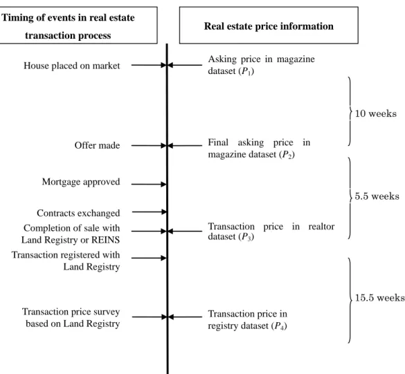
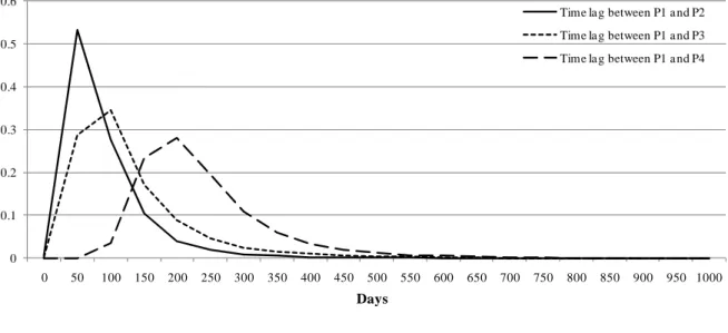
Figure 1 shows the timing at which each of the four prices, P¹, P², P³, and P⁴, is observed in the house buying/selling process in Japan. There is a time lag of 70 days, on average, between the time when P¹is observed (i.e., the time at which a seller posts an initial asking price in the magazine) and the time when P2 is observed (i.e., the time when an offer is made by a buyer and the listing is removed from the magazine). Similarly, there is a lag of 38 days between the time at which P³ is observed (i.e., the time at which a mortgage is approved and a contract is made) and the time at which P² is observed. Finally, there is a lag of 108 days between the time at which P⁴ is observed (i.e., the time at which the MLIT receives price information from a buyer) and the time at which P3 is observed.⁷ In total, the time lag between P1 and P4 is, on average, 216 days, implying that a house price index can be available to the public much earlier by using P1 instead of P4. At the same time, it is often suggested that prices at the earlier stages of the house buying/selling process, such as P¹, are not reliable since they are frequently updated up or down until a final contract price is determined between the buyer and the seller. In addition, it is often pointed out that not all of the prices observed at the earlier stage of the house buying/selling process end in transactions.⁸

Figure 2 shows how time lags are distributed for the four prices. For example, the solid line represents the distribution of the time lag between the day P1 and the day P2 are observed for a particular property. We see that more than fifty percent of all observations are concentrated at a time lag of 50 days, but there is a non-negligible

7According to registry information, the day on which P³is observed and the day on which registration is made at the land registry are identical for 93 percent of all transactions. This means that the time lag between P³ and P⁴ mainly reflects the number of days it takes for the MLIT to collect price information from buyers. Note that this type of time lag does not occur in most other industrialized countries, including the U.S. and the U.K., where the land registry requires sellers and/or buyers to re- port transaction prices as part of the registration information. However, according to Eurostat (2011), even in the U.K., there exists a long time lag regarding the registration of property ownership transfers; that is, registration is typically completed only 4-6 weeks after the completion of transactions. This lack of timeliness means that price information gathered from registration is of limited usefulness in constructing house price indexes.

8Eurostat (2011: 147), for example, notes: “Each source of prices information has its advantages and disadvantages. For example a disadvantage of advertised prices and prices on mortgage applications and approvals is that not all of the prices included end in transactions, and the price may differ from the final negotiated transaction price. But these prices are likely to be available sometime before the final transaction price. Indices that measure the price earlier in the purchase process are able to detect price changes first, but will measure final prices with error because prices can be renegotiated extensively before the deal is finalized.”

(9)

probability that the time lag exceeds 150 days. Similarly, the time lag between P¹ and P4 is most likely to be 200 days, but it is possible, although with a low probability, that it may be more than 300 days.

2.3 Price distributions

Figure 3 shows the cross-sectional distributions for the log of the four prices. The horizontal axis represents the log price while the vertical axis represents the corresponding density. We see that the distributions of P1 and P2 are quite similar to each other. On the other hand, the distribution of P³ differs substantially from the distribution of P²; namely, the distribution of P2 is almost symmetric, while the distribution of P3 has a thicker lower tail, implying that the sample of P3 contains more low-priced houses than the sample of P2. This difference in the two distributions may be a reflection of differences in prices at different stages of the house buying/selling process, but it is also possible that the difference in the price distributions may come from differences in the characteristics of the houses in the two datasets.

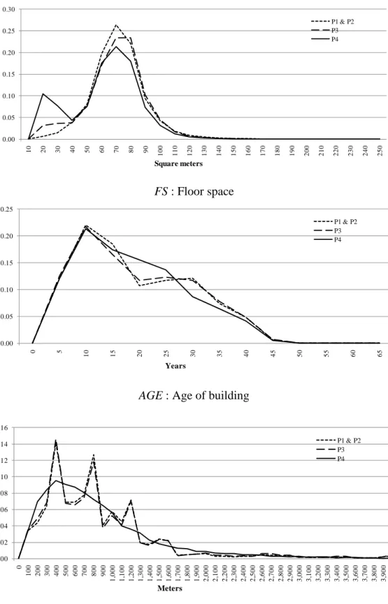
To investigate this in more detail, we compare the distributions of house attributes for each of the three datasets. The top panel of Figure 4 shows the distributions of floor space, measured in square meters, for the three datasets. The distribution labeled “P¹ and P²,” which is from the magazine dataset, is almost symmetric, while the distribution labeled “P3,” which is from the realtor dataset, has a thicker lower tail, indicating that the realtor dataset contains more small-sized houses whose floor space is 30 square meters or less. This pattern is even more pronounced in the registry dataset, i.e., the distribution labeled ”P4.” Turning to the middle and bottom panels of Figure 4, we see that there are substantial differences between the three datasets in terms of the age of buildings and the distance to the nearest station.

These differences in the distributions of house attributes may be related to the differences in the distributions of house prices. More specifically, the different price distributions we saw in Figure 3 may be mainly due to differences in the composition of houses in terms of their size, age, location, etc. Put differently, it could be that the price distributions are identical once quality differences are controlled for in an appropriate manner.

2.4 Quality adjustment

We will adjust for quality in two different ways. For this purpose, let us begin by considering the dataset of initial asking prices in the magazine and the dataset of

(10)

registry prices. We would like to conduct a quality adjustment before comparing the two price distributions. Let F1(p) denote the cumulative distribution function (CDF) of the log of initial asking prices in the magazine and F¹(p | z) denote the conditional CDF of the log of initial asking prices, given a vector of house attributes, z. F1(p) and F1(p | z) are related as follows:

F1(p) =

∫ ∞

−∞

F1(p | z)u1(z)dz (1)

where u¹(z) is the distribution of z for houses in the magazine dataset. Similarly, we define F4(p) and F4(p | z) for the log of registry prices, and u4(z) for houses in the registry dataset. Then we can express the difference between F¹(p) and F⁴(p) as follows: F1(p) − F4(p) =

∫ ∞

−∞

[F1(p | z) − F4(p | z)]u1(z)dz +

∫ ∞

−∞

F4(p | z)[u1(z) − u4(z)]dz (2) The conditional distribution of prices given z can be interpreted as the distribution of quality adjusted prices, so that the first term on the right hand side of eqn. (2) represents the difference between the two distributions of quality adjusted prices. Ac- cording to eqn. (2), however, the difference between F1(p) and F4(p) also comes from differences in terms of the distribution of z between the two datasets (i.e., the magazine dataset and the registry dataset), which is represented by the second term on the right hand side. Our aim is to eliminate the second term before comparing the two price distributions.

Intersection approach The first method to do so is to use prices only for houses that are in both the magazine and the registry datasets. We will refer to this as the “intersection approach.” We use address information to identify these houses. The number of houses in this intersection sample turns out to be 15,015. Since the distributions u¹(z) and u⁴(z) are identical in the intersection sample, eqn. (2) becomes

F1(p) − F4(p) =

∫ ∞

−∞

[F¹(p | z) − F4_{(p | z)]u}1(z)dz. (3) This is how we eliminate the effect of quality differences between datasets.

Note that this method is based on the same idea as the repeat sales method, which is extensively used in constructing quality adjusted house price indexes. As is often pointed out, however, repeat sales samples may not necessarily be representative samples, because houses that are traded multiple times may have some special characteristics that set them apart from other houses. A similar type of sample selection bias may

(11)

arise in our intersection approach. Houses in the intersection between the magazine dataset and the registry dataset are cases which successfully ended in a transaction. In other words, houses whose initial asking prices were listed in the magazine but which failed to get an offer from buyers, or where potential buyers failed to get approval for a mortgage, are not included in the intersection. If such unsuccessful transactions occur randomly, then this would not pose a problem. However, if unsuccessful transactions are more frequent for, say, high-priced houses, this would give rise to sample selection bias, since the distribution of initial asking prices and that of registry prices will differ. Quantile hedonic approach The second method for quality adjustment is based on quantile hedonic regression. Let Q^θ_i(p | z) denote the θ-th quantile of the conditional distribution Fi(p | z), where θ ∈ (0, 1). Following Machado and Mata (2005), we model these conditional quantiles by

Q^θ_i(p | z) = zβi(θ) (4)

This simply states that the conditional quantiles are a weighted average of various house attributes. This is similar to the idea of hedonic regressions, but differs from them in that the weight vector, βi(θ), is assumed to depend on the value of θ. The restriction that hedonic coefficients do not depend on quantiles may not be problematic as long as one is interested in the mean or in the median of the distribution of quality adjusted prices, but it is a serious problem when one is interested in the shape of the entire distribution of quality adjusted prices. We will eliminate this restriction by employing quantile hedonic regression. Note that the weight vector βi(θ), which is referred to as the quantile regression coefficient, can be interpreted as the shadow price associated with each of the house attributes.

Given this setting, we proceed as follows. We first apply quantile regression to initial asking prices and house attributes in the magazine dataset to obtain the estimate of β¹(θ), which is denoted by ˆβ¹(θ). Given the values of z and p, we are then able to calculate F1(p | z) using the equation p = z ˆβ1(θ). The estimate of F1(p | z) is denoted by ˆF¹(p | z). Similarly, we obtain the estimate of F⁴(p | z), denoted by ˆF⁴(p | z), using the registry dataset. By integrating out z, we obtain the estimates of the marginal distributions as follows:

Fˆ1(p) ≡

∫ ∞

−∞

Fˆ1(p | z)u1(z)dz; F^ˆ4(p) ≡

∫ ∞

−∞

Fˆ4(p | z)u4(z)dz (5)

(12)

Then we have an equation analogous to eqn. (2): Fˆ1(p) − ˆF4(p) =

∫ ∞

−∞

[_ˆ

F1(p | z) − ˆF4_{(p | z)]u}1(z)dz +

∫ ∞

−∞

Fˆ4_{(p | z)[u}1(z) − u4_(z)]dz

(6) We use the second term on the right hand side as the difference between the two distributions of quality adjusted prices.

Specifically, we estimate the distribution of quality adjusted prices closely following the method developed by Machado and Mata (2005), consisting of the following steps: 1. Estimate quantile regressions for Q values of θ. The estimates are ˆβ¹(θ) for the

magazine dataset and ˆβ4(θ) for the registry dataset.

2. Draw with replacement from the Q sets of quantile regression coefficient vectors. The individual draws are denoted by ˆβ1(b) and ˆβ4(b), where b = 1, . . . , B. A uniform distribution is used, i.e., each θ is equally likely to be drawn.

3. Draw with replacement from z1_j and z4_k, where z1_j is the vector of explanatory variables for observation j in the magazine dataset (j = 1, . . . , n1), and z4_k

is the vector of explanatory variables for observation k in the registry dataset (k = 1, . . . , n4). Each observation is equally likely to appear in the new vectors, z¹b and z⁴b, b = 1, . . . , B.

4. Calculate z1_bβ^ˆ¹(b), z4_bβ^ˆ⁴(b), and z1_bβ^ˆ⁴(b).

5. Estimate the density functions for z1_bβ^ˆ¹(b), z4_bβ^ˆ⁴(b), and z1_bβ^ˆ⁴(b). The estimates correspond to ˆF1(p), ˆF4(p), and ^∫_−∞^∞ F^ˆ4(p | z)u1(z)dz.

Machado and Mata (2005) use this method to decompose the change of the wage distribution over time into several factors, while McMillen (2008) was the first to apply this method to a cross-sectional house price distribution. Specifically, he decomposed the change in the house price distribution in Chicago between 1995 and 2005 into two components: the change in the distribution of house attributes and the change in the coefficients on the house attributes (i.e., the shadow prices associated with the attributes). His main finding is that the change in the price distribution over time comes mainly from the change in the coefficients on house attributes rather than the change in the distribution of house attributes. These two studies employ this method to investigate the difference between two distributions (i.e., wage distributions or house price distributions) at time t and at time t + 1. The present study differs from these

(13)

two papers in that we compare two distributions that come from different datasets rather than two distributions at different points in time from the same dataset.

3 Empirical Results

3.1 The distribution of quality adjusted prices: Results based on the intersection approach

The magazine dataset, which contains P¹ and P², and the registry dataset, which contains P4, have 15,015 observations in common. On the other hand, there are 22,613 observations in the intersection of the realtor dataset, which contains P³, and the registry dataset, which contains P4. We will use these two intersection samples to estimate the distance between the distributions of prices at different stages of the house buying/selling process.

We start by looking at the distribution of relative prices between P1 and P4 and between P² and P⁴ for housing units in the intersection of the magazine and registry datasets. Similarly, we look at the distribution of relative prices between P3and P4 for housing units in the intersection of the realtor and registry datasets. Figure 5 shows that the distribution of P1/P4 has the largest density at a range of 1.05 to 1.10, with more than thirty percent of the total observations being concentrated in this range, and that the densities above 1.10 are not negligible. In contrast, the number of houses for which P4 exceeds P1 is very limited, indicating that initial asking prices tend to be higher than registry prices. This may reflect the weak housing demand in the period from 2005 to 2009 when the price data was collected. Turning to the relative price P2/P4, the densities for the range of 1.00 and 1.05, and the range of 1.05 and 1.10, are slightly higher than those for the relative price P¹/P⁴, indicating that final asking prices listed in the magazine tend to be closer to registry prices than initial asking prices. This tendency is more clearly seen for the relative prices between realtor prices and registry prices: more than 70 percent of observations are concentrated in the range of 1.00 to 1.05 for P3/P4.

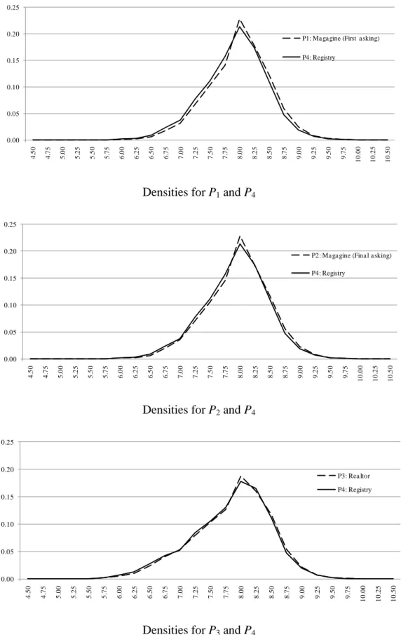
Next, Figure 6 shows the distribution of prices using the intersection samples. The top panel compares the distributions of P1 and P4 using the intersection sample of the magazine and registry datasets. In Figure 3, we saw that the distributions of P1 and P4 are quite different. However, we now find that the difference between the two distributions is much smaller than before, clearly showing the importance of adjusting for quality. However, the two distributions are not exactly identical even

(14)

after the quality adjustment. Specifically, the distribution of P⁴ has a thicker lower tail than the distribution of P1. This may be interpreted as reflecting the fact that asking prices initially listed in the magazine were revised downward during the house selling/purchase process.

The middle panel in Figure 6 compares the distributions of P2 and P4 using the intersection sample of the magazine and registry datasets, while the bottom panel compares the distributions of P3 and P4 using the intersection sample of the realtor and registry datasets. Both panels show that the differences between the distributions are much smaller than we saw in Figure 3, but there still remain some differences.

In order to see how close the distributions of the four prices are, we draw quantile- quantile (q-q) plots, which provide a graphical technique for determining if two datasets come from populations with a common distribution. The q-q plots are shown in Figure 7, where the quantiles of the first set of prices are plotted against the quantiles of the second set of prices. If the two sets of prices come from populations with the same distribution, the dots should fall along 45 degree reference line. The greater the departure from this reference line, the more this suggests that the two sets of prices come from populations with different distributions.

The panels in Figure 7(a) show the q-q plots for raw prices, the distributions of which were shown in Figure 3. The top panel shows the result for P1 and P4, with the log of P⁴ on the horizontal axis and the log of P¹ on the vertical axis. Similarly, the middle and bottom panels show the results for P2 and P4 and for P3 and P4. The three panels all show that the dots are not exactly on the 45 degree line. For example, in the top panel, the dots are above the 45 degree line; moreover, they deviate more from the 45 degree line for low price ranges, indicating that the distribution of P4 has a thicker lower tail than P¹. A similar deviation from the 45 degree line can be seen in the q-q plot for P2 vs. P4 and the q-q plot for P3 vs. P4, although the deviation is smaller in the case of P3 vs. P4 than in the other two cases.

Turning to the q-q plots for quality adjusted prices by the intersection approach, which are presented in Figure 7(b), we see that the dots are much closer to the 45 degree line than before, although there still remains some deviation from the 45 degree line.

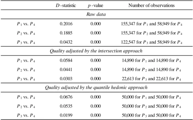
To conduct a formal test to determine if the two distributions come from populations with the same distribution, we calculate the D statistic, which measures the deviation between the two distributions and is defined as follows:

D = max

c ^{| F}^x^{(c) − F}^y^{(c) |} ⁽⁷⁾

(15)

where Fx(·) and Fy(·) are cumulative distributions for two random variables. The estimated D’s are shown in Table 2. The results for the raw data are presented in the first three rows, while the results for the quality adjusted data using the intersection approach are shown in the next three rows. For example, concerning the distributions of P1 and P4, the estimate of D is 0.2016 for the raw data, indicating that the two cumulative distributions deviate a substantial 20 percent. On the other hand, the estimate of D for the quality adjusted data employing the intersection approach is 0.0584, much smaller than the corresponding value for the raw data. However, this does not necessarily mean that the two distributions are the same. In fact, we find that the p-value obtained from the Kolmogorov-Smirnov test (KS test) is very close to zero, implying that the null hypothesis that the two distributions are identical can be easily rejected not only for the raw data but also for the quality adjusted data. We also find that D = 0.0441 for the distributions of P² and P⁴, and D = 0.0303 for the distributions of P3 and P4, implying that the deviation from the distribution of registry prices, P⁴, becomes smaller and smaller at later (i.e., downstream) stages of the house buying/selling process, although the null hypothesis is still rejected for these cases.

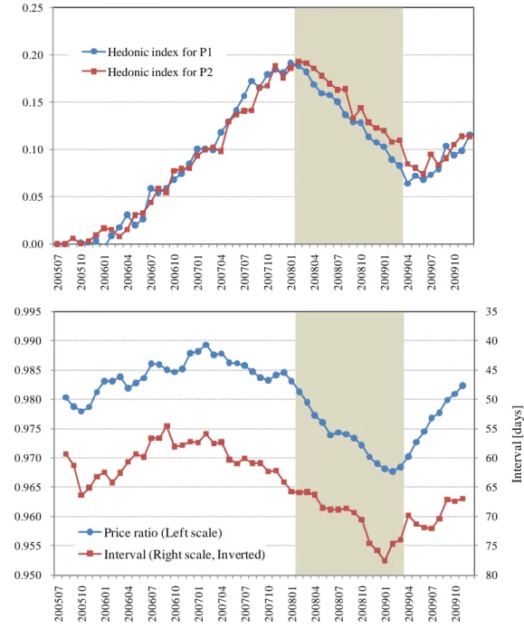
One may wonder how the deviations between the four prices fluctuate over time. In particular, an important question to be asked is whether the deviations differ depending on whether the housing market is in a downturn or in an upturn. To address this, we present in Figure 8 a time series for the price ratio between P1 and P2, as well as a time series for the interval between the time when P1 is observed (i.e., the time at which a seller posts an initial asking price in the magazine) and the time when P² is observed (i.e., the time when an offer is made by a buyer and the listing is removed from the magazine).

The price ratio for a particular month is defined and calculated as the average of the ratios between P2and P1 for housing units for which an offer is made in that month and for which an initial asking price P¹ was listed in the magazine some time prior to that month. As shown in the lower panel of Figure 8, the price ratio fluctuates between 0.97 and 0.99, indicating that P² tends to be lower than P¹ by one to three percent. More importantly, we see that fluctuations in the price ratio are closely correlated with the overall price movement in the housing market, which is represented by the hedonic indexes for P¹ and P² shown in the upper panel of Figure 8. Specifically, the hedonic index for P1 declined by more than ten percent during the period between March 2008 and April 2009 indicated by the shaded area. During this downturn period, the price

(16)

ratio exhibited a substantial decline, and more interestingly, changes in the price ratio preceded changes in the hedonic indexes. Specifically, the price ratio started to decline in December 2007, three months earlier than the hedonic index for P¹, and bottomed out in February 2009, two months earlier than the hedonic index for P1.

Next, the interval for a particular month is calculated as the average of the time lags between the time P2 is observed and the time P1 is observed for those housing units for which an offer is made in that month. The interval fluctuates between 55 and 78 days, and more importantly, it is closely correlated with the hedonic indexes for P¹ and P2. Focusing on the downturn period, which is indicated by the shaded area, we see that the interval increased from 65 days to 78 days, suggesting that, due to weak demand, sellers had to wait longer until an offer is made by a buyer. As in the case of the price ratio, changes in the interval tended to precede changes in the hedonic indexes; specifically, the interval peaked in December 2008, four months before than the hedonic index for P1 hit bottom.

3.2 The distribution of quality adjusted prices: Results based on the quantile hedonic approach

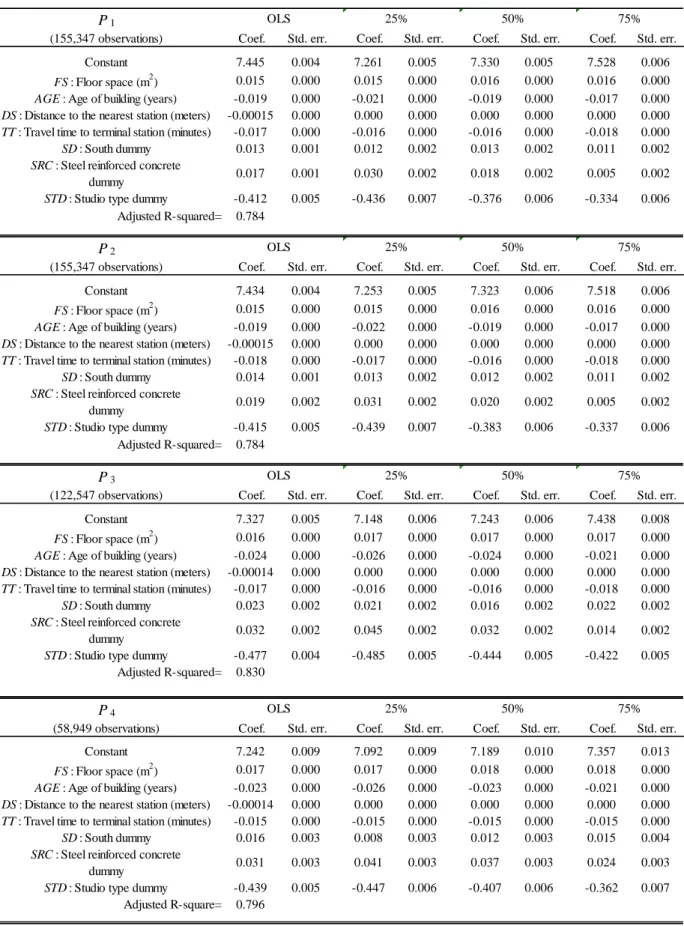
We first conduct a standard hedonic regression for (the log of) the four prices using a similar specification as the one adopted by Shimizu et al. (2010) and others. A list of the variables used in the regression is provided in Table 3. The regression results are shown in the first two columns of Table 4. The results are standard: house prices increase with floor space and decline with age, distance to the nearest station, and commuting time to the central business district; in addition, prices are higher for houses with main windows facing south, and for houses with a steel reinforced concrete frame structure. There are some differences across the four prices in the estimated coefficients, but they are not very large. Each of the four regressions explains more than 70 percent of the variation in the log of house price.

To conduct the Machado-Mata (2005) decomposition, we run 97 quantile regressions for quantiles ranging from θ = 0.02 to 0.98 in increments of 0.01. Table 4 shows the estimates for representative (25 percent, 50 percent, and 75 percent) quantiles, while Figure 9 shows the regression coefficients by quantile. We see that several variables exhibit significant quantile effects. Specifically, the estimated coefficient on the age of a building is negative but tends to become closer to zero at higher quantiles, implying that age decreases house prices, but less so for high-priced houses. The coefficient on the distance to the nearest station is close to zero for quantiles above 90

(17)

percent, indicating that the distance to the nearest station is a less important deter- minant of price for high-priced houses. There is a similar tendency for the coefficient on commuting time to the central business district. On the other hand, we see no significant quantile effects for floor space; that is, the coefficient on floor space does not change much at different quantiles.

Comparing the estimated coefficients for the four prices, we do not see any significant differences. For example, the coefficient on age differs between the four prices in that it is closer to zero for P¹and P²than for the other two prices, but the difference is not statistically significant. Similarly, the coefficient on floor space is smaller (closer to zero) for P1 and P2 than for the other two prices, but the difference is not very large. Based on the results from the quantile hedonic regressions, we decompose the difference between price distributions into two components: the difference resulting from differences in quantile regression coefficients, and the difference resulting from differences in house attribute distributions. For each of the four prices, we make 50,000 independent draws from the vectors of house attributes and 50,000 independent draws from the estimated quantile coefficient vectors. We then use the results to estimate the density functions for z_ibβ^ˆ_i(b) and z_ibβ^ˆ4(b) for i = 1, 2, 3, 4.

The results of this exercise are presented in Figure 10. The top, middle, and bottom panels respectively show the results for the difference between P1 and P4, between P2

and P⁴, and between P³ and P⁴. The solid lines show the difference between the two price distributions, while the dashed lines show the difference due to differences in the quantile hedonic coefficients and the difference due to differences in the distribution of house attributes. For example, the solid line in the upper panel represents ˆf¹(p)− ˆf⁴(p), where ˆfi(p) is the estimated density function whose CDF is given by ˆFi(p). The dashed line labeled “coefficients” in the top panel represents the contribution of differences in the quantile hedonic coefficients, which is given by

∫ ∞

−∞

[_ˆ

f¹(p | z) − ˆf⁴(p | z)]u¹(z)dz

where ˆf_i(p | z) is the estimated conditional density function whose CDF is given by Fˆi(p | z), while the dashed line labeled “variables” in the top panel represents the contribution of differences in the distribution of house attributes, which is given by

∫ ∞

−∞

fˆ4(p | z)[u1(z) − u4(z)]dz.

The solid and dashed lines in the other two panels are similarly defined.

(18)

The top panel of Figure 10 shows that the difference between the distributions of (the log of) P1 and P4 mainly comes from differences in the distribution of house attributes. However, differences in the quantile hedonic coefficient also make a certain contribution. In other words, there remain non-trivial differences between the price distributions even after prices are quality adjusted using the quantile hedonic approach. In the middle and bottom panels, the contribution of differences in the quantile hedonic coefficients becomes smaller but still seems to be non-negligible.⁹

Next, we again use q-q plots to see how close the distributions are. The top panel in Figure 7(c) compares the distribution of quality adjusted values of (the log of) P1, which are defined by ^∫_−∞^∞ f^ˆ1(p | z)u1(z)dz, and the distribution of quality adjusted values of (the log of) P4, which are defined by ^∫_−∞^∞ f^ˆ4(p | z)u1(z)dz. The other two panels in Figure 7(c) compare the distribution of quality adjusted values for P2 and P4

and for P³ and P⁴. We see in the top and middle panels that the dots are located above the 45 degree line, especially at lower quantiles, indicating that there remains some difference between the price distributions even after quality differences are controlled for by quantile hedonic regression. On the other hand, we see little deviation from the 45 degree line in the bottom panel showing the q-q plot for P3 and P4.

Finally, we conduct KS tests to determine if the price distributions come from populations with a common distribution. The results are presented in the bottom three rows of Table 2. The estimated values of the D statistic are D = 0.0676 for the distributions of P1 and P4, D = 0.0535 for the distributions of P2 and P4, and D = 0.0199 for the distributions of P3 and P4, suggesting that the distance between the price distributions tends to be smaller when two sets of prices come from closer stages of the house buying/selling process. However, the p-values associated with the three KS tests are all very close to zero, implying that the null hypothesis that the price distributions come from populations with a common distribution is easily rejected even after prices are quality adjusted using the hedonic quantile approach.¹⁰

9These results are quite different from the ones reported by McMillen (2008), who compared two price distributions, one for 1995 and the other for 2005, and found that virtually the entire difference between the price distributions was due to differences in the quantile hedonic coefficients. Note, however, that McMillen (2008) compared price distributions from different years, while we compare price distributions from different stages of the house buying/selling process, and therefore from different datasets compiled by different parties.

10Note that the quality adjustment using the intersection approach tends to produce lower estimates of the D statistic than the quality adjustment using the quantile hedonic approach. For example, the estimate of D for P¹ vs. P⁴ is 0.0584 for the intersection approach but 0.0676 for the quantile hedonic approach. As discussed earlier, quality adjustment using the intersection approach may suffer from sample selection bias because of unsuccessful transactions (i.e., some houses are listed in the magazine, but not recorded in the registry dataset, for example, because the potential buyer was

(19)

4 Conclusion

In constructing a housing price index, one has to make at least two important choices. The first is the choice among alternative estimation methods. The second is the choice among different data sources of house prices. The choice of the dataset has been regarded as critically important from the practical viewpoint, but has not been discussed much in the literature. This study sought to fill this gap by comparing the distribution of prices collected at different stages of the house buying/selling process, including (1) asking prices at which properties are initially listed in a magazine, (2) asking prices when an offer is eventually made, (3) contract prices reported by realtors, and (4) registry prices. These four prices are collected by different parties and recorded in different datasets. We found that there exist substantial differences between the distributions of the four prices, as well as between the distributions of house attributes. However, once quality differences are controlled for by employing quantile hedonic regressions as proposed by Machado and Mata (2005), there remain only small differences between the price distributions. This suggests that prices collected at different stages of the house buying/selling process are still comparable, and therefore useful in constructing a house price index, as long as they are quality adjusted in an appropriate manner.

[To be completed]

References

[1] Eurostat (2011), Handbook on Residential Property Price Indices, Draft Version 3.0, January 2011. Available at

http://epp.eurostat.ec.europa.eu/portal/page/portal/hicp/methodology/ owner occupied housing hpi/rppi handbook.

[2] McMillen, D. P. (2008), “Changes in the distribution of house prices over time: Structural characteristics, neighborhood, or coefficients?” Journal of Urban Eco- nomics 64, 2008, 573-589.

[3] Koenker, R. (2005), Quantile Regression. Cambridge Univ. Press, New York.

unable to obtain a mortgage). In other words, the intersection samples contain prices only from very homogeneous (maybe excessively homogeneous) houses.

(20)

[4] Koenker, R. and K. F. Hallock (2001), “Quantile regression,” Journal of Economic Perspectives 15, 2001, 143-156.

[5] Machado, J. A. F. and J. Mata (2005), “Counterfactual decomposition of changes in wage distributions using quantile regression,” Journal of Applied Econometrics 20, 445-465.

[6] Ohnishi, T., T. Mizuno, C. Shimizu, and T. Watanabe (2010), “On the evolution of the house price distribution,” Research Center for Price Dynamics Working Paper Series No. 61, August 2010.

[7] Pollakowski, H. O. (1995), “Data sources for measuring house price changes,” Journal of Housing Research 6(3), 377-387.

[8] Shimizu, C., K.G. Nishimura, and T. Watanabe (2010), “Housing prices in Tokyo: A comparison of hedonic and repeat-sales measures,” Journal of Economics and Statistics, Volume 230, Issue 6, Special issue on “Index Theory and Price Statis- tics” edited by Erwin Diewert and Peter von der Lippe, December 2010, 792-813.

(21)

Table 1: Summary of the three datasets

Magazine data (P1, P2)

Mean Std. Dev. Min. Max.

Magazine data (155,347 observations)

P1: First asking price (10,000 Yen) 2,958.51 1,875.16 200 33,000 P2: Final asking price (10,000 Yen) 2,889.27 1,831.34 200 29,800

Log P1: Log of P1 ^7.84 ^0.54 ^5.77 ^10.40

Log P2: Log of P2 ^7.82 ^0.54 ^5.77 ^10.30

FS : Floor space (m²) ^66.77 ^18.97 ^10.39 ^243.90

P1 / FS (10,000 Yen) 43.59 21.65 10.87 195.68

P2 / FS (10,000 Yen) 42.58 21.16 10.00 189.08

AGE : Age of building (years) 16.59 10.26 1.50 58.93

DS : Distance to the nearest station (meters) 850.42 729.86 80 9,900

TT : Travel time to terminal station (minutes) 20.97 12.61 2 89

Realtor data (P3)

Realtor data (122,547 observations)

P3: Sales price (10,000 Yen) 2,431.81 1,632.88 160 29,074

Log P3: Log of P3 ^7.60 ^0.64 ^5.08 ^10.28

FS : Floor space (m²) ^64.87 ^20.27 ^10.10 ^238.81

P3 / FS (10,000 Yen) 37.44 19.65 10.00 187.96

Registry data (P₄)

Registry data (58,949 observations)

P4: Sales price (10,000 Yen) 2,316.32 1,633.34 130 28,000

Log P4: Log of P4 ^7.53 ^0.68 ^4.87 ^10.24

FS : Floor space (m²) ^57.52 ^23.58 ^10.09 ^196.46

P4 / FS (10,000 Yen) 41.38 21.53 10.00 189.83

(22)

Table 2: Goodness-of-fit tests

D -statistic p -value Number of observations

P1 vs. P4 0.2016 0.000 155,347 for P1 and 58,949 for P4

Raw data

Quality adjusted by the intersection approach

Quality adjusted by the quantile hedonic approach

(23)

Table 3: List of variables

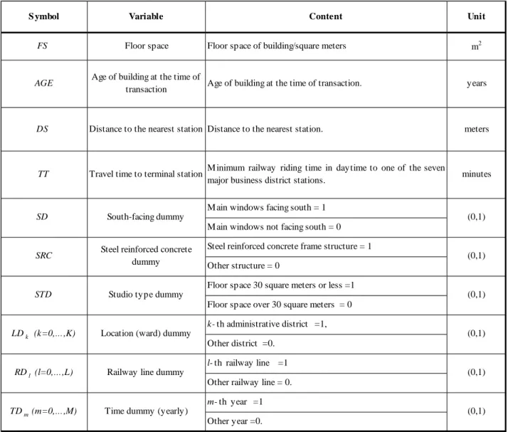
S ymbol Variable Content Unit

FS Floor space Floor space of building/square meters _m²

AGE Age of building at the time of

transaction Age of building at the time of transaction. years

DS Distance to the nearest station Distance to the nearest station. meters

TT Travel time to terminal station M inimum railway riding time in daytime to one of the seven

major business district stations. ^minutes

M ain windows facing south = 1 M ain windows not facing south = 0 Steel reinforced concrete frame structure = 1 Other structure = 0

Floor space 30 square meters or less =1 Floor space over 30 square meters = 0 k- th administrative district =1,

Other district =0. l- th railway line =1

Other railway line = 0. m- th year =1 Other year =0.

SD South-facing dummy (0,1)

SRC Steel reinforced concrete

dummy ^(0,1)

STD Studio type dummy (0,1)

LD_k (k=0,…,K) Location (ward) dummy (0,1)

RD_l (l=0,…,L) Railway line dummy (0,1)

TD_m (m=0,…,M) Time dummy (yearly) (0,1)