A uthor(s )
Poulidis, A lexandros P.; T akemi, T etsuya; Iguchi, Masato;
R enfrew, Ian A .
C itation
J ournal of Geophysical R esearch: A tmospheres (2017),
122(17): 9332-9350
Is s ue D ate
2017-09-16
UR L
http://hdl.handle.net/2433/227302
R ig ht
©
2017 A merican Geophysical Union.; T he full-text file will
be made open to the public on 26 March 2018 in accordance
with publisher's 'T erms and C onditions for S elf-A rchiving'.
T ype
J ournal A rticle
T extvers ion
publisher
Orographic effects on the transport and deposition of volcanic
ash: A case study of Mount Sakurajima, Japan
Alexandros P. Poulidis1 , Tetsuya Takemi1 , Masato Iguchi2 , and Ian A. Renfrew3
1Disaster Prevention Research Institute, Kyoto University, Uji, Japan,2Disaster Prevention Research Institute, Kyoto University, Sakurajima, Japan,3Centre for Ocean and Atmospheric Sciences, School of Environmental Sciences, University of East Anglia, Norwich, UK
Abstract
Volcanic ash is a major atmospheric hazard that has a significant impact on local populations and international aviation. The topography surrounding a volcano affects the transport and deposition of volcanic ash, but these effects have not been studied in depth. Here we investigate orographic impacts on ash transport and deposition in the context of the Sakurajima volcano in Japan, using the chemistry-resolving version of the Weather Research and Forecasting model. Sakurajima is an ideal location for such a study because of the surrounding mountainous topography, frequent eruptions, and comprehensive observing network. At Sakurajima, numerical experiments reveal that across the 2–8� grain size range, the deposition of “medium-sized” ash (3–5�) is most readily affected by orographic flows. The direct effects of resolving fine-scale orographic phenomena are counteracting: mountain-induced atmospheric gravity waves can keep ash afloat, while enhanced downslope winds in the lee of mountains (up to 50% stronger) can force the ash downward. Gravity waves and downslope winds were seen to have an effect along the dispersal path, in the vicinity of both the volcano and other mountains. Depending on the atmospheric conditions, resolving these orographic effects means that ash can be transported higher than the initial injection height (especially for ash finer than 2�), shortly after the eruption (within 20 min) and close to the vent (within the first 10 km), effectively modifying the input plume height used in an ash dispersal model—an effect that should be taken into account when initializing simulations.1. Introduction
Volcanic eruptions introduce large amounts of tephra (i.e., volcanic ash) into the atmosphere, creating a major environmental hazard. Even a small amount of volcanic ash (>2 mg m−3) [Langmann et al., 2012] is a hazard for international aviation, capable of causing major disruptions [Bonadonna et al., 2012]. After deposition, it can directly affect life, livelihoods (destroying crops and pastures), and infrastructure, for example, by caus-ing roof and buildcaus-ing collapses, damagcaus-ing and disruptcaus-ing electricity networks, cloggcaus-ing drainage systems, and contaminating water supplies [Wilson et al., 2012;Hampton et al., 2015]. In the long term, in cities near active volcanoes, ashfall can also have an indirect effect: exacerbating preexisting respiratory conditions [Baxter et al., 1999;Horwell and Baxter, 2006;Hillman et al., 2012], causing psychological stress, and impos-ing the economic burden of regular clean-up and maintenance of vulnerable infrastructure [Wilson et al., 2015]. Accurate prediction of the transport and deposition of ash is therefore vitally important for hazard management and mitigation.
The transport and sedimentation of volcanic ash are complex processes, with the residence time and fall velocity of ash depending critically on its size [Carey and Sparks, 1986;Bonadonna et al., 1998]. Coarse vol-canic ash (>1 mm in diameter) is deposited quickly after an eruption and within a few tens of kilometers from the vent in a largely predictable manner [Carey and Sparks, 1986;Bonadonna et al., 1998;Beckett et al., 2015]. “Medium-sized” ash (diameters between 63μm and 1 mm) stays airborne for more time and is thus more influenced by the local and regional wind field. “Fine” ash (<63μm) stays airborne for longer periods of time: from days (as in the case of the 2010 Eyjajallajökull, Iceland, eruption; [Webley et al., 2012]) to years (e.g., the 1991 Mount Pinatubo, Philippines, eruption) [McCormick et al., 1995]. The deposition of fine ash is still an open research topic, but deposition through aggregation (the joining of airborne ash particles) is widely accepted to exert first-order control [Bonadonna et al., 2012;Brown et al., 2012;Beckett et al., 2015].
RESEARCH ARTICLE
10.1002/2017JD026595Key Points:
• Gravity waves and downslope winds affect the transport and deposition of volcanic ash
• Meteorological-ash-dispersion modeling using WRF is able to resolve orographic process that leads to enhanced ash deposition • The prescribed model plume height
can be modified by orographic effects such as gravity waves near the volcano
Supporting Information:
• Supporting Information S1 • Table S1
Correspondence to:
A. P. Poulidis,
Citation:
Poulidis, A. P., T. Takemi, M. Iguchi, and I. Renfrew (2017), Orographic effects on the transport and deposition of volcanic ash: A case study of Mount Sakurajima, Japan,J. Geophys. Res. Atmos.,
122, 9332–9350, doi:10.1002/ 2017JD026595.
Received 8 FEB 2017 Accepted 16 JUL 2017
Accepted article online 21 JUL 2017 Published online 6 SEP 2017
The atmospheric flow can control both the transport of ash particles via wind dispersal and the deposition. For example, cases of “forced deposition” of volcanic ash occur due to the formation of gravitational instabilities in the plume and/or orographically induced flows or waves, leading to strong downward advection. This can be achieved in at least two ways: via a localized increase in ash concentration, a process primarily controlled by plume dynamics [Manzella et al., 2015], and while the plume traverses complex topography and is impacted by orographic effects in the lee of mountains [Watt et al., 2015]. Precipitation, also a result of the particular atmospheric flow in a given day, has a direct effect on the deposition of volcanic ash and gases by hydrometeor scavenging, i.e., wet deposition [Kawaratani and Fujita, 1990;Witham et al., 2005].
An orographic flow is the result of atmospheric flow responding to isolated mountains or mountain ranges. Depending on a number of factors relating to the mountain topography, atmospheric stability, and wind speed, this interaction creates a variety of flow phenomena both on the windward side—such as flow stagna-tion and splitting—and in the lee—such as lee vortices, gravity (ormountain) waves, hydraulic jumps (abrupt upward displacement of air), and downslope winds [Smith, 1980;Smolarkiewicz and Rotunno, 1989;Durran, 1990;Elvidge et al., 2016]. The Froude number (Fr =U∕(NH), whereU(m s−1) is the incoming flow speed,N (s−1) is the Brunt-Väisälä frequency, andH(m) is the height of an obstacle), is commonly used to characterize a flow based on expected orographic effects: broadly speaking a value less than 1 indicates a nonlinear “flow around” regime with flow splitting and lee vortices, while a value over 1 indicates a linear “flow over” regime with mountain wave activity [Smith, 1980]. Resolving orographic flows is essential for a large number of mete-orological impacts, such as intense rainfall, floods, avalanches, and wildfire prediction [Meyers and Steenburgh, 2013]. The very few relevant studies on the influence of these processes on ash transport have drawn similar conclusions [Watt et al., 2015].
In this study we examine the impact of orographic effects on ash transport and deposition, in the con-text of the Sakurajima volcano in Japan using observational ashfall data and numerical modeling with a meteorological-ash-dispersal model. The localized nature of the dispersal around Sakurajima allows us to study the deposition using unprecedented horizontal and vertical resolution simulations. The paper is orga-nized as follows. Initially, observational data showing the effect of orographic forcing on ash deposition will be examined (sections 2.1 and 2.2). The rest of the study focuses on the eruption of 18 August 2013 (introduced in section 2.3). The modeling setup (section 3) and a validation against observational data (section 4) are presented. Then the impacts of orographic effects are discussed in detail in section 5 and the conclusions in section 6.
2. Observed Features of Ashfall
2.1. The Sakurajima Volcano’s Activity and Observations
Sakurajima (peak height 1117 m) is one of Japan’s most active and closely monitored volcanoes, located on the island of Kyushu, southwestern Japan (Figure 1). The frequent activity of the volcano (currently∼80 events per month releasing approximately 500 kt of ash [Iguchi, 2016]) and a high population density have motivated several studies revealing the effect of the volcano on the well-being of the surrounding communities [e.g.,
Wakisaka et al., 1978;Yano et al., 1985, 1990;Uda et al., 1999;Samukawa et al., 2003;Horwell, 2007;Hillman et al., 2012]. Historically, the volcano had two main craters, Kitadake to the north (the earliest crater) and Minami-dake to the south (Figure 1c). Activity in the volcano started again in 1955 mainly via the MinamiMinami-dake crater. The latest eruptive phase, marked by vulcanian eruptions (i.e., moderate-sized, short-lived eruptive bursts) [Morrissey and Mastin, 2000] from the newly formed Showa crater to the south, started sporadically in 2008, with fairly constant activity since 2009 (see Figure S1 in the supporting information). Most eruptions are weak, but stronger eruptions with plume heights (HP) over 3 km (above ground level, agl) occur approximately every 5–6 weeks. In the latest eruptive phase, the tallest plume height reported has been 5 km agl in August 2013.
Figure 1.(a) Location of the Sakurajima volcano (SKJ) in Japan. Purple squares indicate the three WRF model domains. (b) Map of the Kagoshima prefecture, with Kagoshima (KG), the Kirishima mountain, and other points of interest, as well as tephrameter (orange), and Automated Meteorological Data Acquisition System stations (AMeDAS; blue). Coastline data are shown with black contours, and topography contours are shown for every 300 m between 100 and 1600 m (dark to light green contours). Coastline is shown using the global, self-consistent, hierarchical, high-resolution shoreline data [Wessel and Smith, 1996], and topography contours are based on a digital elevation map (DEM) from the Advanced Spaceborne Thermal Emission and Reflection Radiometer (ASTER) mission [Yamaguchi et al., 1998]. (c) Three-dimensional rendering of Sakurajima and the surrounding topography from Google Earth.
Ashfall from the Sakurajima volcano has been monitored by the Kagoshima prefectural government since 1978 [Iguchi, 2016]. Tephrameters are used to measure ashfall at 62 locations (Figure 1b), daily for some sta-tions within approximately 20 km from the vent and monthly otherwise. The JMA monitors erupsta-tions by recording, for example, eruption time, plume height, and dispersal direction (for an example see Table S1). The eruption plume height is estimated using a combination of weather radar data from Fukuoka and Tanegashima (to the north and south, respectively) and visual data from a camera near the volcano [Shimbori et al., 2013a]. A meteorological station provides data on the vertical structure of the atmosphere (for example, temperature, wind, and stability) is in operation at Kagoshima [31.55∘N/130.55∘E, World Meteoro-logical Organisation code: 47827] with rawinsondes launched twice daily [at 0900 and 2100 Japan standard time (JST = UTC + 9)].
2.2. Observational Evidence of Orographic Forcing
The variation of ash thickness (and by extension ashfall amount) is a key diagnostic for estimating the erupted volume of ash [Daggitt et al., 2014]. In the case of the Sakurajima volcano, average monthly ashfall has been shown to decrease by an inverse power law with distance from the vent [Iguchi et al., 2013;Iguchi, 2016], following
wa=wM(D∕D0)−k, (1)
wherewa(in kg m−2) is the volcanic ash weight,Dis the distance (in km),D
0is a reference distance used for nondimensionalization (1 km), and on a logarithmic plane,wM(in kg m−2) is the intercept, andkis the slope [Iguchi, 2016]. The slope parameter (typically between 2 and 3 for Sakurajima) depends on the atmospheric conditions during the eruptions, such as the wind speed. The intercept coefficient,wM, can be taken as an estimate for the ashfall at a distance of 1 km from the vent.
Figure 2.(a–c) Topography profiles at three cross sections west of the Sakurajima volcano. Markers indicate relevant tephrameter stations. Actual station height is shown by the dashed line. (d) August 2013 ashfall data over the Kagoshima prefecture for tephrameter groups along cross sections (CS) at different angles: CS90 (diamonds), CS108 (squares), CS130 (downward triangles), and others (circles). The Showa vent is marked with an upward triangle. (e–g) Ratio of observed to theoretical ashfall for the lee tephrameter stations along: CS90 (Figure 2e), CS108 (Figure 2f ), and CS130 (Figure 2g). Black markers denote the August 2013 data points. Whisker diagrams of the lee ashfall ratio values versus lee station distance from the vent.
impinges on a mountain) [Houze, 2012] add a degree of complexity that makes a study of monthly data over-complicated. Thus, a subset of “dry” months are studied here. The criteria for selection are as follows: (i) months that featured at least one eruption with a plume height over 1 km dispersing toward the west or northwest and (ii) no rainfall observed west of the volcano for 6 h after the eruption (i.e., while the ash cloud is being advected over the land) in 90% of the eruptions of that month. For (i) JMA observations on the plume height and dispersal were used, while for (ii) hourly rainfall data from two rain gauge stations west of Sakurajima were used. This limited the study to 33 months (46% of the total period).
In the analysis we used data from three groups of stations: directly west (cross section 90, referred to here as CS90; diamond markers), west-northwest (CS108; square markers), and northwest (CS130; triangle markers) of the vent. The location of each station is shown in Figure 2d, while the topography profile along each cross section and the distance of relevant tephrameter stations is shown in Figures 2a–2c. The stations in each group are approximately aligned from the Showa crater so are expected to be affected by the same eruptions.
An increase in ashfall in the lee of a mountain is expected as a result of orographically forced deposition [Watt et al., 2015]. For the case of Sakurajima we focused on the lee side of the Satsuma Peninsula, west of the vol-cano; specifically on the three most distal stations (shown with larger symbols in Figures 2a–2d). Orographic effects over the volcano not studied at this point, as ash from the large number of weak eruptions that occur every month, are expected to affect proximal ash deposits.
that expected with this derived power law slope (k) value are shown in Figures 2e–2g. Values over 1 (100on the figure) indicate a departure from negative power law behavior, which is interpreted here as evidence of orographic processes modifying ash transport and deposition.
Overall orographic enhancement is most clearly noted for CS90; however, all groups show large scatter in the results. On average observed values are 23% larger (dash-dotted line) than the theoretically expected values. For most of the months under study ratio values are over 1, with the most extreme case showing a 100-fold increase. This effect is weaker for CS108 (overall average is close to 1), with almost half of the months sug-gesting increased deposition. Finally, the effect is further weakened for CS130 (average 66% of the theoretical value), suggesting no orographic enhancement on average. The lee ashfall ratio results are summarized with a box and whiskers plot in Figure 2h. In all cases the distribution shows orographic enhancement, i.e., a larger tail at higher ratios, with cases of sixtyfold enhancement even for groups CS108 and CS130.
Although cases of possible orographic enhancement exist for all groups, there is a large number of months when this process seems to be negligible. This can occur for a number of reasons. Probably, the most impor-tant one was mentioned previously: the effect of the topography would not appear explicitly in cases of weaker eruptions from which ash does not reach the lee stations. This would affect the ratio negatively and is expected to be exacerbated depending on the distance of the lee station, as seen here (Figure 2h). Atmo-spheric stability will also affect the results as atmoAtmo-spheric instability weakens gravity waves and thus affects deposition. Finally, in the case of CS130, the lee station is located in a valley between two mountains. Depend-ing on the state of the atmosphere, this can also create interference patterns [e.g.,Grubiši´c and Stiperski, 2009] that could weaken (or enhance) the effect. Further analysis is limited by the monthly nature of the data.
For the remainder of this study we focus on the month of August 2013 and specifically on the 18 August erup-tion as it has been the largest eruperup-tion to date of the current eruptive phase and the atmospheric structure on the day points toward the presence of orographic effects. Note that the August 2013 event is atypical mete-orologically, leading to significant orographic enhancement along the CS108 line and no effect on the CS90 line (Figures 2e–2g). This is due to the meteorological conditions on the day.
2.3. The 18 August 2013 Eruption
On the 18 August 2013 Sakurajima erupted at 1631 JST (0731 UTC) with the plume height estimated between 5 and 7 km agl, based on the Kagoshima airport and JMA weather Doppler radars, respectively [JMA, 2013;
Shimbori et al., 2013b]. Ash was advected W-NW, with ashfall recorded as far as the Koshikijima islands, 90 km in the west (Figure 2c). The ash cloud can be seen moving toward a NW direction in in the Multifunctional Trans-port Satellite (MTSAT-2) data (see Figure S2). The eruption was monitored by the Kagoshima airTrans-port Doppler radar in the north, a JMA weather Doppler radar on SKJ [Shimbori et al., 2013b], and an X-band radar in the city of Tarumizu to the southeast of the volcano [Maki et al., 2016].
This was the largest eruption since 2006, and even though it only lasted for a few minutes, it released an estimated 334±33 kt, equivalent to almost a month’s worth of average ash emissions [seeIguchi, 2016]. We focus on this case for numerical simulations of the transport and deposition of the ash, in order to provide further insight on the orographic effects that appear to have affected the deposition.
3. Model Configuration and Experimental Design
Simulations of the 18 August 2013 eruption were carried out using the Weather and Research Forecasting (WRF) model [Skamarock et al., 2008], version 3.6.1, coupled with “online” chemistry and aerosol calcula-tions (WRF-chem) [Grell et al., 2005]. WRF features a fully compressible, three-dimensional nonhydrostatic atmosphere, with the governing equations solved in flux form (Appendix A1).
3.1. Domain and Parametrization Options
For representing the complex topography of the Kyushu island nested domains were utilized (Figure 1a). The outermost domain (grid spacing ofΔx = Δy = 12.5km, 100×100 grid points) includes the islands of Kyushu and western Honshu. The intermediate domain (Δx = Δy = 2.5km, 125×150 grid points) is centered over Kyushu. The innermost domain (Δx= Δy =0.5km, 300×300 grid points; Figure 1b) is cen-tered over Sakurajima and includes the Kagoshima prefecture and the Koshikijima islands and is used for all figures shown. In the control simulations, referred to here as“normal” topography simulations, the Global 30 arc sec elevation (GTOPO30)—a 30’’ (≃800 m at this latitude) digital elevation map (DEM) data set—is used [Skamarock et al., 2008], with a minimal amount of smoothing to ensure numerical stability of the model for these high-resolution experiments with very steep terrain [Zhong and Chow, 2013]. In order to study the impact of the topography and resolved orographic effects, additional“flat” topography simulationswere car-ried out over a domain with almost zero topography (i.e., topographic height was divided by 1 km in all three domains, leading to a maximum topographic height of∼1 m). There are 90 levels in the vertical with a vertical grid spacing of 50 m in the lowest 2 km. The model top is at approximately 20 km (50 hPa). The out-ermost domain boundaries are specified using the European Centre for Medium-Range Weather Forecasts Interim Re-Analysis data set [Dee et al., 2011], which has been used in the past for similar ash dispersal studies [Macedonio et al., 2016]. The boundaries for the inner domains use one-way nesting. The model is initialized at 0900 JST 18 August 2013 and run for 24 h. The first∼7 h of the simulations are spent on model “spin-up” (approximately 3 h) and waiting for the eruption time (1631 JST). A suite of physical parametrizations (radiation, microphysics, surface layer, and fluxes) is used (see Table S3 for details). Sensitivity tests using different microphysics and planetary boundary layer schemes were carried out, but the results remained qualitatively unchanged.
Note that the 500 m grid size of the innermost domain cannot sufficiently resolve all turbulent motion [Bryan et al., 2003;Takemi and Rotunno, 2003] and falls within the “turbulence gray zone” or “terra incog-nita”: turbulence is neither entirely parameterized nor resolved by a large eddy simulation scheme, which can lead to the neglection of potentially important terms in subfilter-scale turbulence models [Wyngaard, 2004]. Although this is not ideal, due to computational restraints, it is current practice in a number of mesoscale studies [e.g.,Kirshbaum and Durran, 2004;Minder et al., 2013;Cécé et al., 2014;Kirshbaum and Fairman, 2014;
Nugent et al., 2014].
3.2. Source Parameter Specification
The ability of any Volcanic Ash Transport Model (VATM) to produce a realistic ash transport and deposition pat-tern hinges on the determination of appropriate source parameters for the volcano and the eruption [Mastin et al., 2009;Bonadonna et al., 2012]. While requirements vary with each model, WRF requires plume height (from the surface;HP), grain size distribution (GSD), eruptive mass rate (Ṁ; here 1.11×10⁶kg s−1), eruption duration (dE; here 5 min), and the eruption time (tE; 1631 JST). Here most of these parameters are well con-strained with data either provided from the JMA (HP,tE) or estimated by the Sakurajima Observatory of the Disaster Prevention Research Institute, Kyoto University [Ṁ,d
E;Iguchi, 2016].
The plume height (HP) is known to be affected by atmospheric stability [Tupper et al., 2009]. Here we use three differentHPvalues (3, 4, and 5 km agl) in order to test sensitivity of the vertical development of the plume height to the atmospheric structure as well as the overall impact in the ash deposition results.
The GSD is the most difficult source parameter to constrain, as several samples at different distances from the vent are required to create a representative distribution [Bonadonna and Houghton, 2005]. In the case of Sakurajima this can be especially challenging due to the fact that explosive eruptions can occur along with passive degassing on a single day. Due to these difficulties,Mastin et al.[2009] assigned “default” source parameters for 1535 volcanoes (the majority of the Holocene volcanoes), including Sakurajima. Here we used the “Silicic, brief” profile inMastin et al.[2009] which focuses on medium to light ash (between 2 and 7� the distribution is 0.09, 0.22, 0.23, 0.21, 0.18, and 0.07) and has a default duration of 6 min which is close to the eruption studied here. Note that�refers to the Krumbein scale:�= −log2(d d−1
0 ), where�(or “phi”) is the grain size,dis the particle size in millimeters, andd0is a reference size (1 mm). Although the grain size is a dimensionless number,�is commonly used as a unit to avoid confusion. Finally, note that particle aggregation [Costa et al., 2010] is not included in the simulations. At its current state WRF does not support any volcanic ash aggregation parameterizations; however, they are currently being implemented (M. Stuefer, personal communication, 2016). Note that the treatment of the volcanic ash, plume distribution details, and settling law used here is described in further detail in Appendix A.
4. Model Result Validation
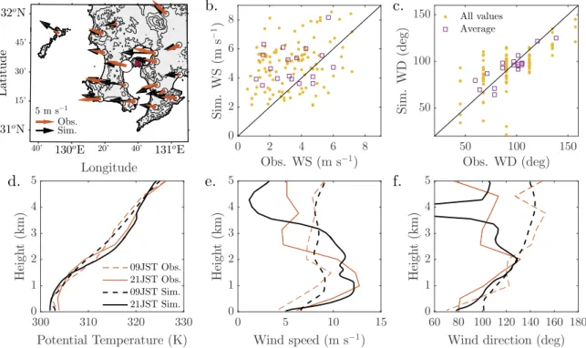
4.1. Atmospheric FlowSurface observations (at 6–10 m) on the 18 August 2013 show atmospheric flow to the W-NW (Figure 3a). There are, however, several deviations from the average flow, indicating the influence of the topography; for example, the station to the north of the Kirishima mountain in the north of the domain (at approximately 32∘N, 131∘E), shows flow to the NW, suggesting flow splitting on the windward side of the mountain, and to a lesser degree at the Osumi Peninsula in the south (between 31∘15′N–31∘25′N and 130∘40’–131∘E), flow
turns to the W-SW suggesting channeling.
In general, the simulated surface flow is in good agreement with Automated Meteorological Data Acquisi-tion System (AMeDAS) observaAcquisi-tions, although for both instantaneous and 6 h average values, WRF tends to overestimate weak winds (Figure 3b): simulated surface wind is higher by a factor of 1.5–3 forU< 3m s−1 and corresponds better for stronger winds (Figure 3b). This is a known issue over complex topography and is thought to occur due to poorly resolved topographic features for atmospheric models, in general [Hanna and Yang, 2001], and WRF, in particular [Jiménez and Dudhia, 2012, 2013]. The root-mean-square error (RMSE) is 2.44 m s−1for instantaneous and 2.24 m s−1for hourly data. The wind direction correspondence is gen-erally good: for instantaneous values the RMSE is 18.95∘, while for 6 h averages this is further reduced to 9.74∘(Figure 3c). In the case of both wind speed and wind direction RMSEs are within the expected range mentioned byHanna and Yang[2001].
A comparison with rawinsonde observations over Kagoshima shows that the model is able to capture impor-tant characteristics of the vertical structure of the atmosphere (Figures 3d–3f ). The potential temperature profiles match well, although the model produces a more stably stratified boundary layer (0–2 km; Figure 3d). The model captures the complex wind shear characteristics with some small deviations; specifically, the sim-ulated decrease of wind speed occurs at a higher point (between 2 and 3 km instead of 2 km), and the model underestimates the minimum wind speed at a height of 4 km (1.2 compared to 5 m s−1). The wind direction profiles (Figure 3f ) are closely matched for the lowest 5 km with the exception of a relatively thin layer between 3.5 and 4.2 km, where there are very low wind speeds (another known WRF issue) [Jiménez and Dudhia, 2013].
The mountainous topography of the Kyushu island introduces significant orographic effects in the atmo-spheric flow as simulated in the WRF model (Figure 4). This is consistent with orographic flow theory as the Froude number for the case ranged between 1.1 and 1.35, indicating a flow over regime and the presence of gravity waves but with some flow splitting possible [Smith, 1980]. Note that Froude number was calculated upwind, for flow along the two main wind directions (108∘close to the surface and 130∘at≃4km), from the surface up to 2 km, and for an obstacle similar to Sakurajima (i.e., a height of≃1 km).
Figure 3.Comparison between simulated and observed meteorological data on 18 August 2013. (a) AMeDAS network (Obs.) and WRF (Sim.) averaged surface wind vectors. (b) Scatterplots of simulated wind speed against observational data using all data (yellow) and average values (purple). (c) As in Figure 3b but for wind direction. (d–f ). Observed (orange) and simulated (black) vertical profiles of potential temperature (Figure 3d), wind speed (Figure 3e), and wind direction (Figure 3f ). The vertical profiles shown are for the Kagoshima meteorological station (large marker size in Figure 3a).
the flow over the volcano introducing alternating areas of strong ascent (in red) and descent (in blue). Close to the surface (up to a height of 1 km), strong downslope winds develop (up to 12.9 m s−1), approximately 1.6 times larger than the 0–2 km layer average (7.8 m s−1). The influence of the gravity waves is visible in the vertical structure of the wind fields up to 4–5 km in height to a distance of 40–50 km to the west at CS108 (Figure 4e) and continues beyond 60 km for CS130, enhanced by new activity over the Satsuma Peninsula mountains (between−20and−30km in Figure 4f ). Note that the potential temperature lines (isentropes; brown lines Figures 4e and 4f ) are parallel to the flow (as indicated by the wind vectors) as potential tem-perature is conserved for adiabatic motions. For this reason isentropes will subsequently be used to display flow lines.
At a height of 4 km from the surface, the flow to the west of Sakurajima is southeasterly with considerably lower horizontal wind speeds to the NW of the volcano, especially over the land (Figure 4b). At this level, strong gravity wave activity can be identified in the southern part of the island by the alternating bands of blue and pink after the two ridge-like peninsulas and the Koshikijima islands.
Overall the WRF model is able to provide a reasonably realistic representation of the atmospheric flow on the day of the eruption. There is good agreement between simulated and observed wind direction. A num-ber of orographic effects are resolved by the fine resolution of the simulations. Although the observational network around Sakurajima and the Kirishima mountain is not dense enough to capture detailed orographic flows in observations, the flow that was resolved by the model is as theoretically expected and there is good agreement between simulated and observed wind direction. On the other hand, comparison of simulated and observed wind speed shows larger disagreements; close to the surface low wind speeds are overestimated by the model, possibly due to subgrid topographic effects, a known issue for the model [Jiménez and Dudhia, 2012, 2013]. Finally, enhanced mountain wave activity due to the increased stability in the model will need to be kept in mind when discussing ashfall results.
4.2. Ashfall
Figure 4.Simulated atmospheric flow for 18 August 2013. (a and b) Vertical velocity (shaded) and horizontal wind vectors at the surface (10 m) (Figure 4a), 4 km (Figure 4b) above the surface. (c and d) As in Figures 4a and 4b but focused over the west of Sakurajima. (e and f ) Horizonal cross section of vertical velocity (shaded) with wind vectors and isentropes plotted every 2 K between 298 and 334 K. Cross-section lines are shown as lines in Figure 4a, green (CS108) for Figure 4e, and red (CS130) for Figure 4f. All results are averaged between 1600 and 2200 JST.
observations as well as radar and satellite data close to the volcano [Shimbori et al., 2013b;Maki et al., 2016]. Deposition occurs along two clearly defined branches in all cases. This is due to the shear in the vertical wind profile, with the two branches corresponding to the wind direction values close to the surface (lower branch; CS108) and aloft (upper branch; CS130). This is illustrated by the change in the patterns with plume height: lower plume heights lead to narrower deposition patterns (i.e., the two branches are closer together and the ashfall area is more limited) with a more pronounced lower branch and ash deposited more homogeneously along the path of the dispersal, while higher plume heights lead to wider deposition patterns with a gap over the Satsuma Peninsula mountains. Overall, results from the normal and flat topography experiments are similar. However, flattening the topography leads to narrower deposition patterns (note the deviation of the upper branch from the wind direction aloft) with more clearly defined edges.
Figure 5.Simulated ashfall for (a–c) normal topography and (d–f ) flat topography simulations. Results shown for different plume heights,HP: 3 km (Figures 5a and 5d), 4 km (Figures 5b and 5e), and 5 km (Figures 5c and 5f ). Ashfall observations are as reported from the JMA for the 18 August 2013. Simulated ashfall is shown at the end of the simulation (17 h after the eruption). Dashed lines mark cross sections CS108 and CS130.
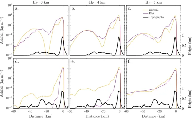
Figure 6 shows that across the southern branch (Figures 6a–6c) the two maxima can be seen in both the normal and flat topography simulations. Field observations of downwind increases in ash deposition (termed secondary thickness maxima) are commonly inferred to arise from particle aggregation, enhancing the rate of ash settling [Carey and Sigurdsson, 1982;Brown et al., 2012;Watt et al., 2015]. Since no aggregation is included in our simulations, the model results suggest that departures from simple downwind patterns of decreasing deposition must be caused primarily by the topography, meteorology, and the depositional patterns of each variable ash bin. Although secondary maxima appear in both simulation types, the simulations that include topography produce a more pronounced secondary depositional maximum and shift this maximum more distally on the lee side of the Satsuma Peninsula.
Ashfall on the day was measured at a small number of locations near the volcano (indicated with diamond markers in Figure 5; also see Table S2). Although the number of the observation points is too small to con-duct meaningful statistical analysis, they can be used for a rudimentary comparison with the model results. On Sakurajima, ashfall was measured at four points close to the coast: in the north (0.25 kg m−2), west (approximately 1 and 4 kg m−2) and the south (0 kg m−2). The observed value at the northern point is only captured well in theHP = 4, 5 km simulations with normal topography. In theHP =3km normal topogra-phy simulation, as well as in all the flat topogratopogra-phy simulations, the depositional pattern is too narrow. The observed values at the points on the west of Sakurajima are captured better in theHP=3, 4 km simulations, as the largest ashfall values shift to the north for theHP=5km simulations. At all of the points on Sakurajima ashfall is underestimated by the model in all simulations; this may be due to the lack of heavier ash that was not included in the GSD set in the model. Finally, over Kagoshima there is one point where recorded ashfall was explicitly 0 kg m−2—in close proximity to locations where ashfall was observed. This (and other similar locations with mixed results in the JMA observational data) could be the result of microscale circulations within the city. Despite the high resolution, such effects are still subgrid scale and not resolved.
Figure 6.Ashfall distribution for the normal topography (yellow line) and flat topography (purple line) at cross sections shown in Figure 5. (a–c) CS108 and (d–f ) CS130 for different plume heights. Topography (black line) shown in all panels to facilitate comparison. Note that the topography is not shown in a logarithmic scale.
in the flat topography simulations, even in cases where there is ashfall over the cross section (for example, Figures 6e and 6f ).
As detailed depositional data are only available very close to the volcano, the simulated ashfall pattern away from the volcano can only be compared to the JMA report for the day [JMA, 2013]. As there is no specified lower limit for the JMA observations, here we use 0.01 kg m−2for the calculations and took the position of each reported point as representative of the corresponding grid point in the model. This allowed us to esti-mate an “accuracy” value (i.e., the percentage of matching points) for each simulation. The overall accuracy of the simulations is between 59 and 62% for the normal topography simulations and 38–55% for the flat topog-raphy simulations. In the former, the best overall accuracy occurs for theHP=5km plume simulation which, although overestimating ashfall northwest of the volcano (i.e., north of the CS130 line), does include matches to the south and west. This is in agreement with the observations of column height. Similar conclusions can be drawn when comparing the simulated ash cloud to satellite data (see Figure S2).
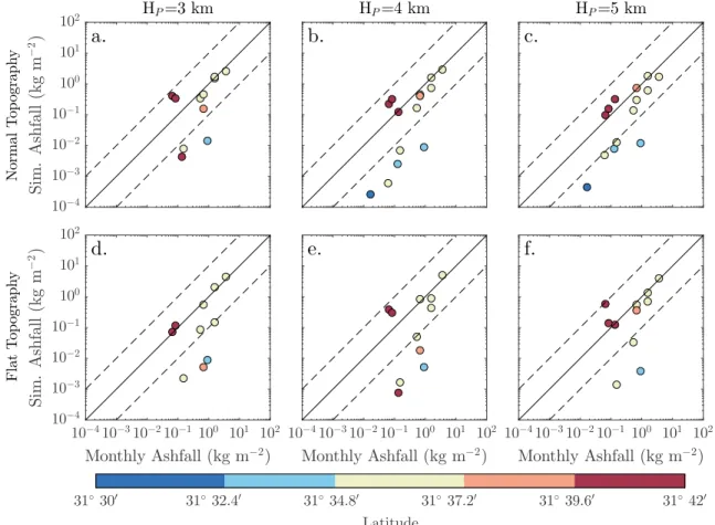
A quantitative comparison of ashfall away from the volcano is also possible, against monthly observations (Figure 7). For August 18 2013 the event was decidedly the largest and most significant eruption (see Table S1), releasing half of the total ash released during the month, and so an order of magnitude comparison is justified. For most stations to the northwest of the volcano (latitudes over 31∘34.8’) simulated ashfall is within an order of magnitude of that observed, i.e., for 50–56% for the normal topography simulations and 46–50% for the flat topography simulations. Ashfall west of the volcano is underestimated in the simulations.
Figure 7.Comparison of simulated ashfall values against monthly tephrameter values for August 2013 for (a–c) normal topography and (d–f ) flat topography simulations and different plume heights. Marker color indicates the latitude of the tephrameter station.
[Iguchi, 2016], and on the day of the eruption the volcano was continuously emitting ash for most of the day. It is possible that ash from these constant emissions and other small eruptions traveled west of the volcano. However, the possibility of model error cannot be ruled out, especially as misrepresentation of wind direction over complex topography is a known issue in the model [Jiménez and Dudhia, 2013].
Other possible sources of discrepancy in the results might stem from the current configuration of the WRF model with respect to volcanic ash. The GSD is known to be an important factor in the final ash deposition patterns [Bonadonna et al., 1998]. Here we assume a “medium” GSD which is an approximation to commonly known GSDs in eruptions of similar scale to the event under study here. Because of the uncertainties in GSD, such discrepancies in the results can be expected. As such results presented here should be viewed as a semiidealized case study rather than an attempt to provide an exact representation of the event.
5. Orographic Processes Affecting Ash Dispersal and Deposition in Sakurajima
Comparison of the normal and flat topography simulations has shown that orography has a significant impact on ash deposition. The resolution of orographic effects has led to an overall increase in the fidelity of the simulation results. Here we will examine these effects in detail by looking at the dispersal of the ash plume. Note that all mentions of heights in this section are above sea level (asl) to avoid confusion when looking at the cross sections in Figures 8–10.
5.1. Orographic Effect Sensitivity by Grain Size
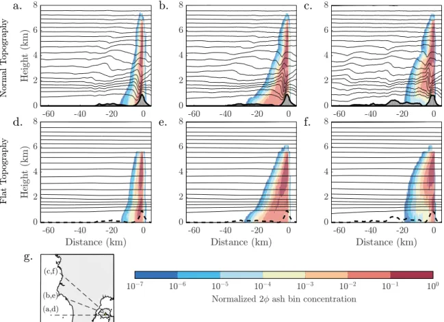
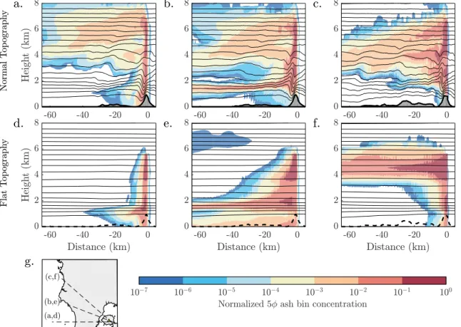
Figure 8.(g) Cross sections of maximum ash concentration (shaded) for the 2�ash bin across the paths for (a–c) normal topography and (d–f ) flat topography. Isentropes (6 h averaged) plotted as contours every 2 K between 298 and 334 K. For all simulationsHP=5km.
concentration value to allow an intercomparison. As the ash cloud moves from east to west without any points of flow reversal (right toward left in the figures), and the eruption duration was short with respect to changes in the wind field, the use of peak concentration provides a summary of the movement of the plume. The potential temperature lines (isentropes) are mean values for 6 h after the eruption and give an indication of the basic atmospheric flow during these 6 h. Due to the stability of the atmosphere, strong gravity wave activity is triggered in the lee of the volcano and in the lee of the Satsuma Peninsula (Figures 8a–8c).
The heaviest ash bin (2�) is the least affected by orographic effects (Figure 8). The most noticeable difference can be seen for the main dispersal axes (Figures 8b and 8e, and 8c and 8f ). Due to gravity wave activity over the volcano, ash is pushed farther up in the atmosphere, reaching over the originally prescribed volcanic plume height top of 6 km to 7.5 km asl. Close to the surface and directly west of the volcano, gravity waves keep ash afloat, reducing ash concentration and forcing ashfall further away.
The impacts of orographic effects are more clearly visible for the 3�ash bin (Figure 9). It is clear that the ash distribution follows the gravity waves, being uplifted in the lee of the volcano and then subsiding farther downwind, so keeping ash afloat close to the volcano and focusing deposition over the lee of the Satsuma Peninsula acting along with the general forced descent due to the topography (compare Figures 9b and 9c to 9e and 9f ). Close to the volcano, downslope winds have an opposing role to the gravity waves, as they push the lowest part of the plume downward, enhancing ashfall over the slopes (for example, Figure 9a). They can also have a more direct effect in the lee of other mountains as seen in Figure 9c where part of the ash cloud is pulled down toward the surface at−60 km.
Figure 9.As in Figure 8 but for the 3�ash bin.
the model, this orographically induced mixing close to the volcano could be enhancing gravitational instabil-ities that lead to proximal deposition of ash [e.g.,Manzella et al., 2015]. Compared to the the flat experiments, there is less ashfall along the first NW direction (Figures 10b and 10e), as ash is trapped in a stratified layer between 1 and 2 km. Another direct effect of gravity wave activity is a large increase in ash concentration aloft (above 4 km asl) not present in the flat topography simulations. Note that lighter ash generally follows the same behavior as the 5�ash bin.
5.2. Volcanic Plume Height
For the finer ash bins shown here (3 and 5�ash bins), the ash is transported significantly higher than the initial plume injection height, due to upward advection by gravity waves. Within the first few minutes of the eruption in both the normal and flat simulations the top of the plume increases by∼1 km due to mixing in the model. In the normal simulation this moves the top of the plume to approximately 7.5 km asl, which is close to the observed top [Shimbori et al., 2013b]. In addition, within the first 30–60 min and within the first 10–20 km from the vent the plume top rises by an additional 1–2 km up to 8.5 km asl. This is due to gravity wave activity occurring close to the volcano, pushing the air flow upward (for example, see between 5 and 8 km height, at−10–0 km in Figures 10b and 10c). This effect is less important for heavier particles that sediment quickly and are deposited within the first 30 min. Although not shown here, a similar increase is noted for theHP=3 and 4 km simulations. This leads to a difference between the prescribed plume height (HPin the present study) and the “effective” plume height (i.e., the maximum plume height simulated in the model over the volcano). An injection height of 6 km asl (i.e.,HP=5 km) led to an increase of approximately 2.5 km, between 1 and 1.5 km over the highest radar-based estimates. An injection height of 5 km asl with a similar increase falls within the radar plume height estimate range, explaining the good performance of the lower plume heights.
Figure 10.As in Figure 8 but for the 5�ash bin.
6. Conclusions
Due to its frequent activity and comprehensive tephrameter network, the Sakurajima volcano provides an ideal natural laboratory for the study of orographic effects on ashfall. An analysis of tephrameter observations shows a clear enhancement of ash deduced to be orographically forced.
High-resolution meteorological-ash-dispersion modeling, capable of resolving complex orographic effects, has shown that the WRF model is able to produce realistic ashfall dispersal and deposition patterns. Medium-sized ash (3–5�) was seen to be the most sensitive to orographic effects. There are counteracting processes with downslope winds and turbulent mixing enhancing ash deposition and gravity waves keeping ash afloat. Resolving orographic effects greatly enhances both horizontal and vertical diffusion of ash in the model. However, it leads to a potential ambiguity over the volcano: due to gravity wave activity over the vol-cano the prescribed “plume height” is elevated by up to approximately 2.5 km, an enhancement that could affect other low plume height eruptions.
Appendix A: WRF-chem as a Volcanic Ash Transport Model (VATM)
The WRF model is a versatile state-of-the-art numerical weather prediction model [Skamarock and Klemp, 2008] that has been used in a number of atmospheric studies, ranging from large eddy simulations of cloud dynamics [e.g.,Kirshbaum and Durran, 2004] to regional climate change studies [e.g.,Mearns et al., 2012]. The inclusion of the chemistry core [Grell et al., 2005] allows for the study of chemical pollutant and aerosol disper-sal [e.g.,Tie et al., 2007], as well as advanced aerosol-cloud interaction [Chapman et al., 2009]. Although use has been mainly constrained to light aerosols (particulate matter 10μm or less in diameter, PM10, and PM2.5), it is possible to use built-in processes for the representation of volcanic ash [Stuefer et al., 2012]. Even though this has been used in a number of cases [e.g.,Webley et al., 2012;Steensen et al., 2013], WRF-chem as a VATM is still at an early stage. For this reason some relevant characteristics of the model are included here for reference.
A1. WRF-Chem Governing Equations
In WRF-chem the transport of all chemical species and aerosols is carried out online, at every time step, using the conservative (flux) form for the integration of prognostic equations [Grell et al., 2005]:
(��)t+ ∇(V��) =0. (A1)
In this equation�is the column mass of dry air,V is the velocity (u,v), and�is a scalar mixing ratio. The model conserves mass and scalar mass exactly due to a finite volume formulation [Lin and Rood, 1996]. A Runge-Kutta third-order time scheme is coupled with a fifth-order evaluation of the horizontal flux diver-gence in the scalar conservation equation and a third-order evaluation of the vertical flux diverdiver-gence [Wicker and Skamarock, 2002]. A positive-definite advection scheme is used for momentum, scalar, turbulent kinetic energy, and chemical species [Skamarock et al., 2008]. In the experiments here, a Rayleigh damping layer is used in the last 5 km before the model top [Klemp et al., 2008].
A2. Volcanic Emissions and Plume
In WRF-chem, the eruption is not explicitely simulated; instead, a volcanic ash plume is inserted manually, in a predefined distribution, up to a specified height at a chosen time and sustained for the duration of the eruption.Poulidis et al.[2016] have shown that volcanic vent heating generates strong convective plumes which locally affect the atmospheric circulation. However, at present an eruption cannot be simulated in the WRF model. The default plume distribution used in WRF is the umbrella shape associated with large eruptions [Sparks et al., 1997], although this can be changed by the user. WRF uses a linear mass distribution beneath the umbrella—25% of the mass is contained in up to 73% of the eruptive column height, and a parabolic mass distribution with 75% of the entrained mass located on the top [Stuefer et al., 2012]:
Ma(h) = ⎧ ⎪ ⎪ ⎨ ⎪ ⎪ ⎩ NL h
Ub ifh
≤Ub
NU [
h−Ub HP−Ub−
(h−U b HP−Ub
)2]
ifUb<h≤HP
0 ifh>HP
(A2)
NL=0.25 Ub ∑
h=0 (
h Ub
)
MT, (A3)
NU=0.75 HP ∑
h=Ub [
h−Ub HP−Ub−
( h−Ub HP−Ub
)2]
MT, (A4)
whereMais the volcanic ash mass at heighth,NL, andNUare the mass beneath and included in the umbrella, respectively (also accounting for the normalization of the mass function),Ubis the umbrella bottom height, HPis the plume height, andMTis the total mass released.
Radiation and Transport model [Chin et al., 2002], based on the Stokes law, modified for volcanic ash radius and density. A Cunningham slip factor was also applied to account for noncontinuum effects for particles with diameters less than 15μm [Pruppacher and Klett, 1997].
References
Baxter, P. J., et al. (1999), Cristobalite in volcanic ash of the Soufrière Hills volcano, Montserrat, British West Indies,Science,283, 1142–1145, doi:10.1126/science.283.5405.1142.
Beckett, F. M., C. S. Witham, M. C. Hort, J. A. Stevenson, C. Bonadonna, and S. C. Millington (2015), The sensitivity of NAME forecasts of the transport of volcanic ash clouds to the physical characteristics assigned to the particles,J. Geophys. Res. Atmos.,120, 11,636–11,652, doi:10.1002/2015JD023609.
Bonadonna, C., G. Ernst, and R. S. J. Sparks (1998), Thickness variations and volume estimates of tephra fall deposits: The importance of particle Reynolds number,J. Volcanol. Geotherm. Res.,81, 173–187, doi:10.1016/S0377-0273(98)00007-9.
Bonadonna, C., and B. Houghton (2005), Total grain-size distribution and volume of tephra-fall deposits,Bull. Volcanol.,67, 441–456, doi:10.1007/s00445-004-0386-2.
Bonadonna, C., A. Folch, S. Loughlin, and H. Puempel (2012), Future developments in modelling and monitoring of volcanic ash clouds: Outcomes from the first IAVCEI-WMO workshop on Ash Dispersal Forecast and Civil Aviation,Bull. Volcanol.,74, 1–10, doi:10.1007/s00445-011-0508-6.
Brown, R. J., C. Bonadonna, and A. J. Durant (2012), A review of volcanic ash aggregation,Phys. Chem. Earth,45–46, 65–78, doi:10.1016/j.pce.2011.11.001.
Bryan, G. H., J. C. Wyngaard, and J. M. Fritsch (2003), Resolution requirements for the simulation of deep moist convection,Mon. Weather Rev.,131, 2394–2416, doi:10.1175/1520-0493(2003)131<2394:RRFTSO>2.0.CO;2.
Carey, S. N., and H. Sigurdsson (1982), Influence of particle aggregation on deposition of distal tephra from the May 18, 1980, eruption of Mount St. Helens volcano,J. Geophys. Res.,87, 7061–7072, doi:10.1029/JB087iB08p07061.
Carey, S., and R. S. J. Sparks (1986), Quantitative models of the fallout and dispersal of tephra from volcanic eruption columns,Bull. Volcanol.,
48, 109–125, doi:10.1007/BF01046546.
Cécé, R., D. Bernard, C. d’Alexis, and J.-F. Dorville (2014), Numerical simulations of island-induced circulations and windward katabatic flow over the Guadeloupe archipelago,Mon. Weather Rev.,142, 850–867, doi:10.1175/MWR-D-13-00119.1.
Chapman, E. G., W. I. Gustafson Jr., R. C. Easter, J. C. Barnard, S. J. Ghan, M. S. Pekour, and J. D. Fast (2009), Coupling aerosol-cloud-radiative processes in the WRF-Chem model: Investigating the radiative impact of elevated point sources,Atmos. Chem. Phys.,9, 945–964, doi:10.5194/acp-9-945-2009.
Chin, M., P. Ginoux, S. Kinne, B. N. Holben, B. N. Duncan, R. V. Martin, J. Logain, A. Higurashi, and T. Nakajima (2002), Tropospheric aerosol optical thickness from the GOCART model and comparisons with satellite and Sun photometer measurements,J. Atmos. Sci.,59, 461–483, doi:10.1175/1520-0469(2002)059<0461:TAOTFT>2.0.CO;2.
Cioni, R., P. Marianelli, R. Santacroce, and A. Sbrana (2000), Plinian and subplinian eruptions, inEncyclopedia of Volcanoes, edited by H. Sigurdsson, pp. 477–494, Academic Press, San Diego, Calif., doi:10.1016/B978-0-12-385938-9.00029-8.
Costa, A., A. Folch, and G. Macedonio (2010), A model for wet aggregation of ash particles in volcanic plumes and clouds: 1. Theoretical formulation,J. Geophys. Res.,115, B09201, doi:10.1029/2009JB007175.
Daggitt, M. L., T. A. Mather, D. M. Pyle, and S. Page (2014), AshCalc—A new tool for the comparison of the exponential, power-law and Weibull models of tephra deposition,J. App. Volcanol.,3, 7, doi:10.1186/2191-5040-3-7.
Dee, D. P., et al. (2011), The ERA-Interim reanalysis: Configuration and performance of the data assimilation system,Q. J. R. Meteorol. Soc.,
137, 553–597, doi:10.1002/qj.828.
Durran, D. R. (1990), Mountain waves and downslope winds,Atmos. Processes Over Complex Terrain, Meteorol. Monogr.,23, 59–81. Eckermann, S., J. Lindeman, D. Broutman, J. Ma, and Z. Boybeyi (2010), Momentum fluxes of gravity waves generated by variable Froude
number flow over three-dimensional obstacles,J. Atmos. Sci.,67, 2260–2278, doi:10.1175/2010JAS3375.1.
Elvidge, A. D., I. A. Renfrew, J. C. King, A. Orr, and T. A. Lachlan-Cope (2016), Foehn warming distributions in non-linear and linear flow regimes: A focus on the Antarctic Peninsula,Q. J. R. Meteorol. Soc.,142, 618–631, doi:10.1002/qj.2489.
Grell, G. A., S. E. Peckham, R. Schmitz, S. A. McKeen, G. Frost, W. C. Skamarock, and B. Eder (2005), Fully coupled “online” chemistry within the WRF model,Atmos. Environ.,39, 6957–6975, doi:10.1016/j.atmosenv.2005.04.027.
Grubiši´c, V., and I. Stiperski (2009), Lee-wave resonances over double bell-shaped obstacles,J. Atmos. Sci.,66, 1205–1228, doi:10.1175/2008JAS2885.1.
Hampton, S. J., J. W. Cole, G. Wilson, T. M. Wilson, and S. Broom (2015), Volcanic ashfall accumulation and loading on gutters and pitched roofs from laboratory empirical experiments: Implications for risk assessment,J. Volcanol. Geotherm. Res.,304, 237–252, doi:10.1016/j.jvolgeores.2015.08.012.
Hanna, S. R., and R. Yang (2001), Evaluations of mesoscale models’ simulations of near-surface winds, temperature gradients, and mixing depths,J. Appl. Meteorol.,40, 1095–1104, doi:10.1175/1520-0450(2001)040<1095:EOMMSO>2.0.CO;2.
Hasegawa, Y., A. Sugai, Y. Hayashi, Y. Hayashi, S. Saito, and T. Shimbori (2015), Improvements of volcanic ash fall forecasts issued by the Japan Meteorological Agency,J. Appied Volcanol.,4(2), 1–12, doi:10.1186/s13617-014-0018-2.
Hillman, S. E., C. J. Horwell, A. L. Densmore, D. E. Damby, B. Fubini, Y. Ishimine, and M. Tomatis (2012), Sakurajima volcano: A physico-chemical study of the health consequences of long-term exposure to volcanic ash,Bull. Volcanol.,74, 913–930, doi:10.1007/s00445-012-0575-3.
Horwell, C. (2007), Grain size analysis of volcanic ash for the rapid assessment of respiratory health hazard,J. Environ. Monit.,9, 1107–1115, doi:10.1039/B710583P.
Horwell, C., and P. Baxter (2006), The respiratory health hazards of volcanic ash: A review for volcanic risk mitigation,Bull. Volcanol.,69, 1–24, doi:10.1007/s00445-006-0052-y.
Houze, R. (2012), Orographic effects on precipitating clouds,Rev. Geophys.,50, RG1001, doi:10.1029/2011RG000365.
Iguchi, M. (2016), Method for real-time evaluation of discharge rate of volcanic ash—Case study on intermittent eruptions at the Sakurajima volcano, Japan,J. Disaster Res.,11, 4–13.
Iguchi, M., T. Tameguri, Y. Ohta, S. Ueki, and S. Nakao (2013), Characteristics of volcanic activity at Sakurajima volcano’s Showa crater during the period 2006–2011,Bull. Volcanol. Soc. Japan,58, 115–135.
Japan Meteorological Agency (JMA) (2013),The Sakurajima Volcano Activity Report, August 2013, Japan Meteorological Agency, Fukuoka, Japan.
Acknowledgments
Jiménez, P. A., and J. Dudhia (2012), Improving the representation of resolved and unresolved topographic effects on surface wind in the WRF model,J. Appl. Meteorol.,51, 300–316.
Jiménez, P. A., and J. Dudhia (2013), On the ability of the WRF model to reproduce the surface wind direction over complex terrain,J. Appl. Meteorol.,52, 1610–1617.
Kanamori, H., J. Mori, and D. G. Harkrider (1994), Excitation of atmospheric oscillations by volcanic eruptions,J. Geophys. Res.,99, 21,947–21,961, doi:10.1029/94JB01475.
Kawaratani, R. K., and S. I. Fujita (1990), Wet deposition of volcanic gases and ash in the vicinity of Mount Sakurajima,Atmos. Environ.,24, 1487–1492, doi:10.1016/0960-1686(90)90057-T.
Kirshbaum, D. J., and D. R. Durran (2004), Factors governing cellular convection in orographic precipitation,J. Atmos. Sci.,61, 682–698, doi:10.1175/1520-0469(2004)061<0682:FGCCIO>2.0.CO;2.
Kirshbaum, D. J., and J. G. Fairman Jr. (2014), Cloud trails past the Lesser Antilles,Mon. Weather. Rev.,143, 995–1017, doi:0.1175/MWR-D-14-00254.1.
Klemp, J. B., J. Dudhia, and A. D. Hassiotis (2008), An upper gravity-wave absorbing layer for NWP applications,Mon. Weather Rev.,136(10), 3987–4004, doi:10.1175/2008MWR2596.1.
Langmann, B., A. Folch, M. Hensch, and M. Volker (2012), Volcanic ash over Europe during the eruption of Eyjajallajökull on Iceland, April–May 2010,Atmos. Environ.,48, 1–8, doi:10.1016/j.atmosenv.2011.03.054.
Lin, S. J., and R. B. Rood (1996), Multidimensional flux-form semi-Lagrangian transport schemes,Mon. Weather Rev.,124, 2046–2070, doi:10.1175/1520-0493(1996)124<2046:MFFSLT>2.0.CO;2.
Macedonio, G., A. Costa, S. Scollo, and A. Neri (2016), Effects of eruption source parameter variation and meteorological dataset on tephra fallout hazard assessment: Example from Vesuvius (Italy),J. App. Volcanol.,5, 1–19, doi:10.1186/s13617-016-0045-2.
Maki, M., M. Iguchi, T. Maesaka, T. Miwa, T. Tanada, T. Kozono, T. Momotani, A. Yamaji, and I. Kakimoto (2016), Preliminary results of weather radar observations of Sakurajima volcanic smoke,J. Disaster Res.,11, 15–28.
Manzella, I., C. Costanza, J. C. Phillips, and H. Monnard (2015), The role of gravitational instabilities in deposition of volcanic ash,Geology,43, 1–4, doi:10.1130/G36252.1.
Mastin, L. G., et al. (2009), A multidisciplinary effort to assign realistic source parameters to models of volcanic ash-cloud transport and dispersion during eruptions,J. Volcanol. Geotherm. Res.,186, 10–21, doi:10.1016/j.jvolgeores.2009.01.008.
McCormick, M. P., L. W. Thomason, and C. R. Trepte (1995), Atmospheric effects of the Mt. Pinatubo eruption,Nature,373, 399–404, doi:10.1038/373399a0.
Mearns, L., et al. (2012), The North American regional climate change assessment program: Overview of phase I results,Bull. Am. Meteorol. Soc.,93, 1337–1362, doi:10.1175/BAMS-D-11-00223.1.
Meyers, M. P., and J. W. Steenburgh (2013), Mountain weather prediction: Phenomenological challenges and forecast methodology, inMountain Weather Research and Forecasting, edited by F. K. Chow, S. F. J. DeWekker, and B. J. Snyder, pp. 1–34, Springer, New York, doi:10.1007/978-94-007-4098-3_1.
Minder, J. R., R. B. Smith, and A. D. Nugent (2013), The dynamics of ascent-forced orographic convection in the tropics: Results from Dominica,J. Atmos. Sci.,70, 4067–4088, doi:10.1175/JAS-D-13-016.1.
Morrissey, M. M., and L. G. Mastin (2000), Vulcanian eruptions, inEncyclopedia of Volcanoes, edited by H. Sigurdsson, pp. 463–476, Academic Press, San Diego, Calif., doi:10.1016/B978-0-12-385938-9.00028-6.
Nugent, A. D., R. B. Smith, and J. R. Minder (2014), Wind speed control of tropical orographic convection,J. Atmos. Sci.,71, 2695–2712, doi:10.1175/JAS-D-13-0399.1.
Poulidis, A. P., and T. Takemi (2017), A 1998–2013 climatology of Kyushu, Japan: Seasonal variations of stability and rainfall,Int. J. Climatol.,
37, 1843–1858, doi:10.1002/joc.4817.
Poulidis, A. P., I. A. Renfrew, and A. J. Matthews (2016), Thermally induced convective circulation and precipitation over an isolated volcano,
J. Atmos. Sci.,184, 1667–1686, doi:10.1175/JAS-D-14-0327.1.
Pruppacher, H. R., and J. D. Klett (1997),Microphysics of Clouds and Precipitation, p. 954, Kluwer Acad., Dordrecht, Netherlands. Samukawa, T., K. Arasidani, H. Hori, H. Hirano, and T. Arima (2003), C-jun mRNA expression and profiling amplification in rat alveolar
macrophages exposed to volcanic ash and sulphur dioxide,Ind. Health.,41, 313–319, doi:10.2486/indhealth.41.313.
Shimbori, T., T. Sakurai, M. Tahara, and K. Fukui (2013a), Observation of eruption clouds with weather radars and meteorological satellites: A case study of the eruptions at Shinmoedake volcano in 2011,Q. J. Seismol.,77, 139–214.
Shimbori, T., A. Takagi, H. Yamauchi, K. Fukui, A. Sugai, Y. Hayashi, Y. Hayashi, Y. Hasegawa, and M. Maki (2013b), The eruption cloud echo from Sakurajima volcano on 18 August 2013 observed by weather radar network, November 2013,Volcanic Eruption Prediction Committee Bull.,116, 253–259.
Shimbori, T., R. Kai, Y. Hayashi, Y. Hayashi, A. Sugai, Y. Hasegawa, A. Hashimoto, A. Takagi, T. Yamamoto, and K. Fukui (2014), Tephra fall predictions with the JMA regional atmospheric transport model: A case study of the eruptions at Shinmoedake volcano in 2011,
Pap. Meteorol. Geophys.,65, 75–107.
Skamarock, W. C., and J. B. Klemp (2008), A time-split nonhydrostatic atmospheric model for weather research and forecasting applications,
J. Comput. Phys.,227, 3465–3485, doi:10.1016/j.jcp.2007.01.037.
Skamarock, W. C., J. B. Klemp, J. Dudhia, D. O. Gill, D. M. Barker, M. G. Duda, X.-Y. Huang, W. Wang, and J. G. Powers (2008), A description of the advanced research WRF version 3, Tech. Rep., NCAR/TN-4751STR.
Smith, R. B. (1980), Linear theory of stratified hydrostatic flow past an isolated mountain,Tellus,32, 348–364, doi:10.1111/j.2153-3490.1980.tb00962.x.
Smolarkiewicz, P. K., and R. Rotunno (1989), Low Froude Number flow past three-dimensional obstacles. Part I: Baroclinically generated lee vortices,J. Atmos. Sci.,46, 1154–1164, doi:10.1175/1520-0469(1989)046<1154:LFNFPT>2.0.CO;2.
Sparks, R. S. J., M. I. Bursik, S. N. Carey, J. S. Gilbert, L. S. Glaze, H. Sigurdsson, and A. W. Woods (1997),Volcanic Plumes, p. 574, John Wiley, Chichester, U. K.
Steensen, T., M. Stuefer, P. Webley, G. Grell, and S. Freitas (2013), Qualitative comparison of Mount Redoubt 2009 volcanic clouds using the PUFF and WRF-Chem dispersion models and satellite remote sensing data,J. Volcanol. Geotherm. Res.,259, 235–247, doi:10.1016/j.jvolgeores.2012.02.018.
Stuefer, M., S. R. Freitas, G. Grell, P. Webley, S. Peckham, and S. A. McKeen (2012), Inclusion of Ash and SO2 emissions from volcanic eruptions in WRF-CHEM: Development and some applications,Geosci. Model Dev.,5, 2571–2597, doi:10.5194/gmd-6-457-2013.
Takemi, T., and R. Rotunno (2003), The effects of subgrid model mixing and numerical filtering in simulations of mesoscale cloud systems,
Mon. Weather Rev.,131, 2085–2101, doi:10.1175/1520-0493(2003)131<2085:TEOSMM>2.0.CO;2.
Tupper, A., C. Textor, M. Herzog, H.-F. Graf, and M. S. Richards (2009), Tall clouds from small eruptions: The sensitivity of eruption height and fine ash content to tropospheric instability,Nat. Hazards,51, 375–401, doi:10.1007/s11069-009-9433-9.
Uda, H., S. Akiba, H. Hatano, and R. Shinkura (1999), Asthma-like disease in the children living in the neighbourhood of Mt. Sakurajima,
J. Epidemiol.,9, 27–31, doi:10.2188/jea.9.27.
Wakisaka, I., A. Takano, and N. Watanabe (1978), Health effects of volcanic ashes of Mt. Sakurajima,Jpn. J. Publ. Health,25, 155–461, doi:10.1080/00039896.1990.10118757.
Watt, S. F. L., J. S. Gilbert, A. Folch, J. C. Phillips, and X. M. Cai (2015), An example of enhanced tephra deposition driven by topographically induced atmospheric turbulence,Bull. Volcanol.,77, 35, doi:10.1007/s00445-015-0927-x.
Webley, P. W., T. Steensen, M. Stuefer, S. Freitas, and M. Pavolonis (2012), Analyzing the Eyjajallajökull 2010 eruption using satellite remote sensing, lidar and WRF-Chem dispersion and tracking model,J. Geophys. Res.,117, D00U26, doi:10.1029/2011JD016817.
Wessel, P., and W. H. F. Smith (1996), A global self-consistent, hierarchical, high-resolution shoreline database,J. Geophys. Res.,101, 8741–8743, doi:10.1029/96JB00104.
Wicker, L. J., and W. C. Skamarock (2002), Time splitting methods for elastic models using forward time schemes,Mon. Weather Rev.,130, 2088–2097, doi:10.1175/1520-0493(2002)130<2088:TSMFEM>2.0.CO;2.
Wilson, T. M., C. Stewart, V. Sword-Daniels, G. S. Leonard, D. M. Johnston, J. W. Cole, J. Wardman, G. Wilson, and S. T. Barnard (2012), Volcanic ash impacts on critical infrastructure,Phys. Chem. Earth,45–46, 5–23, doi:10.1016/j.pce.2011.06.006.
Wilson, T. M., S. F. Jenkins, and C. Stewart (2015), Volcanic ash fall impacts, inGlobal Volcanic Hazards and Risk, edited by S. C. Loughlin et al., pp. 281–288, Cambridge Acad. Press, Cambridge.
Witham, C. S., C. Oppenheimer, and C. J. Horwell (2005), Volcanic ash-leachates: A review and recommendations for sampling methods,
J. Volcanol. Geotherm. Res.,141, 299–326, doi:10.1016/j.jvolgeores.2004.11.010.
Wyngaard, J. C. (2004), Toward numerical modeling in the “terra incognita”,J. Atmos. Sci.,61, 1816–1826, doi:10.1175/1520-0469(2004)061<1816:TNMITT>2.0.CO;2.
Yamaguchi, Y., A. B. Kahle, H. Tsu, T. Kawakami, and M. Pniel (1998), Overview of Advanced Spaceborne Thermal Emission and Reflection Radiometer (ASTER),IEEE Trans. Geosci. Remote Sens.,36, 1062–1071, doi:10.1109/36.700991.
Yano, E., A. Takeuchi, S. Nishii, A. Koizumi, A. Poole, R. C. Brown, N. F. Johnson, P. H. Evans, and Y. Yukiyama (1985), In vitro biological effects of volcanic ash from Mount Sakurajima,J. Toxicol. Environ. Health,16, 127–135, doi:10.1080/15287398509530724.
Yano, E., Y. Yokoyama, H. Higashi, S. Nishii, K. Maeda, and A. Koizumi (1990), Health effects of volcanic ash: A repeat study,Arch. Environ. Health,45, 367–373, doi:10.1080/00039896.1990.10118757.
Zhong, S., and F. K. Chow (2013), Meso- and fine-scale modeling over complex terrain: Parameterizations and applications, inMountain Weather Research and Forecasting, edited by F. K. Chow, S. F. J. DeWekker, and B. J. Snyder, pp. 591–653, Springer,