つくばリポジトリ

(1)

A s t udy on aeol i an dus t out br eak i n Eas t As i a

著者

Kur os aki Yas unor i

内容記述

Thes i s ( Ph. D

. i n Sc i enc e) - - U

ni ver s i t y of

Ts ukuba, ( B) , no. 2040, 2004. 6. 30

I nc l udes bi bl i ogr aphi c al r ef er enc es

発行年

2004

(2)

A Study on Aeolian Dust Outbreak

in East Asia

A Dissertation Submitted to

the Graduate School of Life and Environmental Science,

the University of Tsukuba

in Partial Fulfillment of the Requirements

for the Degree of Doctor of Philosophy in Science

(3)

Abstract

The impact of aeolian dust on climate has been recognized to be large due to radiative effect. Intergovernmental Panel on Climate Change (IPCC) [2001] also treats the aeolian dust as an important factor of climate change. However, the uncertainty of the effect of the aeolian dust is very large and the level of scientific understanding about the aeolian dust is classified as very low in IPCC [2001]. One of the major reasons of insufficient understanding is the inhomogeneous distribution of aeolian dust owing to their short lifetime. They are removed by rain typically within a week. As a result, the concentration of aeolian dust rises to its highest near its source just after its outbreak. The uncertainty still remains due to the difficulty of understanding the distribution of aeolian dust sources and the timing of aeolian dust outbreak.

Aeolian dusts are generated by strong surface winds, while land surface conditions largely affect aeolian dust outbreaks because the threshold wind velocity of aeolian dust outbreak has various values according to land surface conditions. Therefore, it is important to recognize the distribution of aeolian dust sources, land cover types (e.g., desert, grassland, forest, cultivation) around aeolian dust sources and threshold wind velocities according to land surface conditions.

This study focuses on the aeolian dust outbreak in East Asia, which is one of the major aeolian dust sources. The following three geographical characteristics are found

(4)

ii

relatively high latitude. These geographical characteristics make it difficult to understand the spatial and temporal distributions of aeolian dust outbreaks in East Asia.

The purposes in this study are to clarify (i) the relation between aeolian dust sources and land cover types, (ii) which largely control aeolian dust outbreaks, surface winds or land surface conditions, (iii) the spatial distribution of threshold wind velocities of aeolian dust outbreak, and (iv) the effect of snow cover on aeolian dust outbreak. For these purposes, this study conducts statistical analyses by use of surface meteorological data, land cover type data and snow cover data in East Asia for the period from March 1988 to June 2003. Conclusions are summarized as follows:

1. Aeolian dust sources in East Asia distribute in regions of Bare Desert, Semi Desert Shrubs, Grass/Shrub and Cultivation. The northern boundary of dust sources almost corresponds to the southern boundary of the Forest regions. The southern boundary of dust sources distribute around the southern boundaries of Bare Desert and Semi Desert Shrubs regions in middle and upper reaches of the Huang He River.

2. Aeolian dust outbreaks frequently occur at months of frequent strong winds around the Gobi Desert and in the Taklimakan Desert. The months of frequent dust outbreaks are limited in March, April and May around the Gobi Desert, while dust outbreaks frequently occur from March to July and/or August in the Taklimakan

Desert. According to the correlation between strong wind frequency and dust outbreak frequency, the surface wind primarily controls dust outbreaks in March and April. This tendency is strong especially in the Taklimakan Desert. On the other hand, land surface conditions largely affect aeolian dust outbreaks in May around the Gobi Desert.

(5)

both kinds of threshold velocities (i.e., ut5% and ut50%) decrease from the northeast (i.e., Mongolia and Inner Mongolia) to the southwest (i.e., the Taklimakan Desert). From the viewpoint of land cover type, they are the largest in the Grass/Shrub region, the next largest in the Semi Desert Shrubs region and the smallest in the Bare Desert region. Differences of threshold velocity (∆ut = ut50% – ut5%) are large in Mongolia and small in the west of the Taklimakan Desert. This result indicates that land surface conditions are largely variable in Mongolia and almost constant in the west of the Taklimakan Desert.

4. This study statistically analyzed the relation between the threshold wind velocity of dust outbreak and snow cover in March and April. It is found that the threshold velocity linearly increases with snow cover fraction. The threshold velocity is well parameterized with snow cover fraction. This formulation improves the correlation between the strong wind frequency and the dust outbreak frequency in East Asia in March and April.

(6)

iv

List of Tables

Table 2.1. Present weathers in SYNOP associated with aeolian dust phenomena. All kinds of present weathers are presented in Appendix 1. ……… 24 Table 2.2. Definitions about phenomena of aeolian dust. Symbolic letters “ww” identifies

the present weather in a SYNOP report. ……… 25 Table 2.3. Legend of land cover types in this study (left column) and their corresponding

to numbers of the Global Ecosystem Legend (right column). The Global Ecosystem Legend is presented in Appendix 2. ……… 26 Table 4.1. Selected stations in the Taklimakan Desert and region names defined in this

study. ……… 61 Table 4.2. Definitions about phenomena of aeolian dust in section 4.2. Symbolic letters

“ww” identifies the present weather in a SYNOP report (see section 2.1.2). Although dust outbreak corresponds to ww=07, 09, 30-35 and 98 in section 4.2, ww=08 is a member of dust outbreak in other sections (i.e., ww=07, 08, 09, 30-35 and 98). In other words, ww=08 is excluded from the group of dust outbreak in section 4.2. Similar to dust outbreak, ww=08 is not a member of dust event in section 4.2 (see also Table 2.2). ……… 62 Table 4.3. Month of peak for the dust event and the dust outbreak. ……… 63 Table 5.1. Regions (left column) and their major land cover types (right column).

……… 90 Table 6.1. Relation among ∆SWF, ∆DOF, and ∆SCF in each region. ……… 109 Table 6.2. Relations of surface wind velocity (u) with SCF (fsc), when DOF takes values

(10)

viii

List of Figures

Fig. 1.1. A schematic illustration of the three distinct phases of aeolian dust: entrainment, transport and deposition. Atmospheric conditions (flow patterns, precipitation and turbulence), soil characteristics (texture, aggregation and moisture) and land-surface properties (roughness elements and vegetation) control the erosion process (modified from Shao, 2000). ……… 10 Fig. 1.2. Global, annual-mean radiative forcings (Wm-2_{) due to a number of agents for}

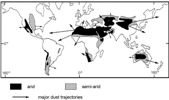
the period from pre-industrial (1750) to present (late 1990s; about 2000). The height of the rectangular bar denotes a central or best estimate value, while its absence denotes no best estimate is possible. The vertical line about the rectangular bar with “x” delimiters indicates an estimate of the uncertainty range, for the most part guided by the spread in the published values of the forcing. A vertical line without a rectangular bar and with “o” delimiters denotes a forcing for which no central estimate can be given owing to large uncertainties. The uncertainty range specified here has no statistical basis and therefore differs from the use of the term elsewhere in this document. A “level of scientific understanding” index is accorded to each forcing, with high, medium, low and very low levels, respectively. This represents the subjective judgment about the reliability of the forcing estimate, involving factors such as the assumptions necessary to evaluate the forcing, the degree of knowledge of the physical/chemical mechanisms determining the forcing, and the uncertainties surrounding the quantitative estimate of the forcing (after IPCC, 2001). ……… 11 Fig. 1.3. Distribution of regions with high dust-storm activity and major dust

trajectories (after Pye, 1987). ……… 12 Fig. 1.4. Wind erosion severity. The different levels of severity were obtained by the

combination of the degree of degradation and the percentage of the area affected (after Middleton and Thomas, 1997). ……… 13 Fig. 1.5. Geographical distribution of the different source types of aeolian dust, and a

boundary condition of aeolian dust outbreaks in the numerical experiment of Tegen and Fung [1995]. ……… 14 Fig. 1.6. Modeled annual dust emission simulated from natural (upper) and disturbed

(lower) soils for the case of 50 % contribution from disturbed soils to the total dust load. The global annual dust emission for each of both source types is 1500 Mt yr-1_{. Results of numerical simulation in}_{Tegen and Fung}_{[1995]. …… 15} Fig. 1.7. The global distribution of TOMS dust sources. This figure is a composite of

(11)

specific dust sources. The distributions were computed using a threshold of 1.0 in the dust belt (see section 1.4.2) and 0.7 everywhere else (after Prospero et al., 2002). ……… 16 Fig. 1.8. Approximate location of the April 19 dust cloud over the Pacific Ocean between April 21 and 25. The daily dust pattern was derived from the SeaWiFS images, GOES 9 and GOES 10 images, and TOMS absorbing aerosol index data. Over the Pacific Ocean the dust cloud followed the path of the springtime East Asian aerosol plume shown by the contours of optical thickness derived from AVHRR data (after Husar et al., 2001). ……… 17 Fig. 1.9. SeaWiFS true color images of the trans-Pacific dust transport from April 20 –

25, 1998. These images are obtained from http://daac.gsfc.nasa.gov/CAMPAIGN_DOCS/OCDST/asian_dust.html. Detail explanations about this episode are also indicated in this homepage.

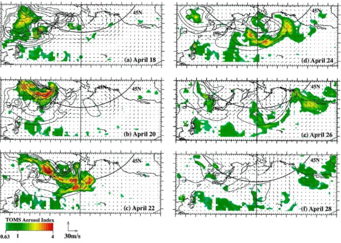
……… 18 Fig. 1.10. Wind vector at z*_{= 1500 m (model output), horizontal distribution of}

column-averaged concentration of dusts shown by contours (model output), and TOMS aerosol index shown by color hatches (satellite observations) for April 18 – 28, 1998, over the North Pacific basin. Dust concentration levels of 1, 2.5, 6.3, 10, 16, 25, 40, and 100µg/m3_{are shown by contour lines (after}_{Uno et al.}_{, 2001).} z*_{is the terrain-following vertical coordinate and this is defined as z}_t_{(z – z}_g_{) / (z}_t – zg), where zt and zg are the levels of the top and the ground surface of the model atmosphere, respectively. ……… 19 Fig. 2.1. The analysis region. Both color hatches and black contour lines indicate

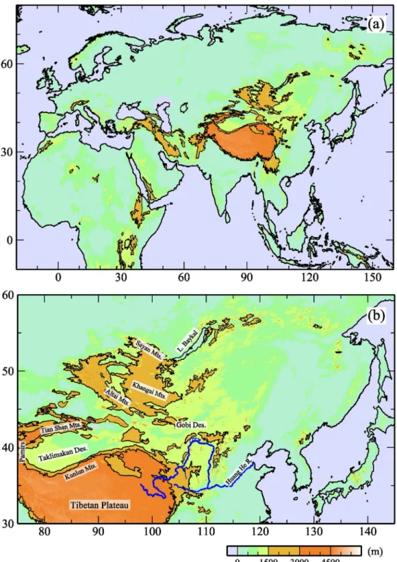
topography. Contour lines indicate coastlines and elevations of 1500 m and 3000 m. Dots show WMO synoptic observatories. Blue lines indicate Huang He River. Red lines indicate national borders. ……… 27 Fig. 3.1. Topography around the global dust belt (a) and East Asia (b). Black solid

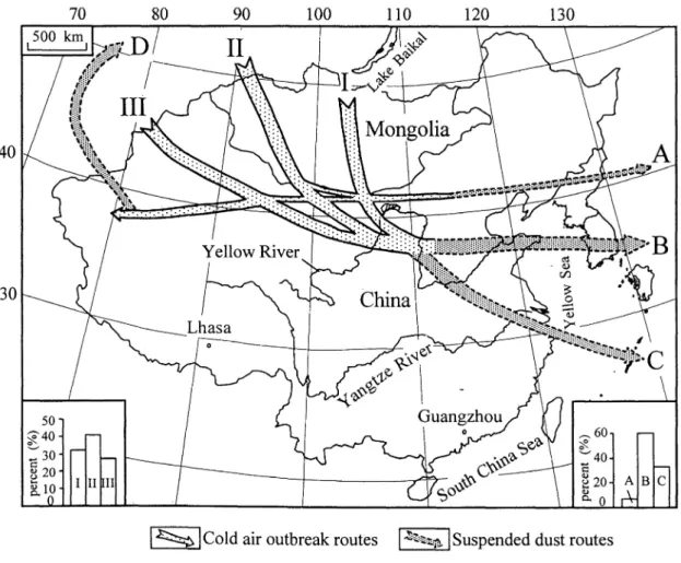
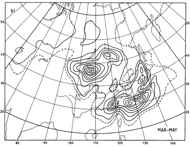
contours indicate coast and elevations of 1500 m A.S.L. and 3000 m A.S.L. ……… 33 Fig. 3.2. Routes of the cold air outbreaks and the dust transport patterns in China (after Sun et al., 2001). ……… 34 Fig. 3.3. Number of cyclogenetic events (10-2_{) per 2.5° quadrangle per month for spring} (March to May) for the period 1958 – 1987 (after Chen et al., 1991).

……… 35 Fig. 3.4. The SeaWiFS true color image of April 16, 1998. White cloud due to a synoptic disturbance and yellow (or brown) cloud of aeolian dusts can be seen from this image. This image is obtained from the following homepage, http://daac.gsfc.nasa.gov/CAMPAIGN_DOCS/OCDST/asian_dust.html.

……… 36 Fig. 3.5. Surface meteorological sites where aeolian dusts were observed at 03 UTC in

(12)

x

the same time. Symbols indicate present weather of SYNOP report (see section 2.1.2). ……… 37 Fig. 3.6. Three-dimensional structure of the dust cloud around the cutoff vortex from

April 16 to 19 over China and Japan. Streamlines on a horizontal plane at 3 km level are plotted in orange, and those on a vertical plane passing through at 32°N and 130°E (from surface to 18 km level) are plotted in white. Dust concentration of 100 µg/m3_{is shown by isosurfaces, and its surface is colored by} the value of potential temperature (after Uno et al., 2001). These are model outputs of Uno et al. [2001]. ……… 38 Fig. 3.7. Time-height cross section of potential temperature (contour, 3° interval) and

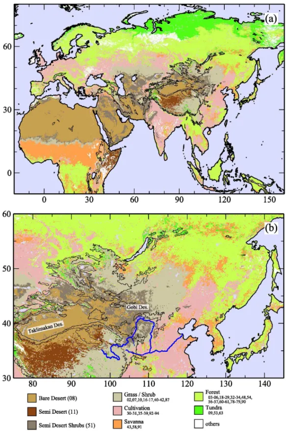
dust concentration (color) at several sites: (a) Qingdao, (b) Khabarovsk, (c) Shanghai, (d) Seoul, (e) Okinawa, and (f) Fukuoka (after Uno et al., 2001). These are model outputs of Uno et al. [2001]. ……… 39 Fig. 3.8. Land cover types around the global dust belt (a) and East Asia (b). Black solid

contours indicate coast and elevations of 1500 m A.S.L. and 3000 m A.S.L. same as Fig. 3.1. Legends should be referred to section 2.2.1. …… 40 Fig. 3.9. Distributions of snow cover in March for 1988 – 2003 (upper panel), in April for

1988 – 2003 (middle panel) and in May for 1988 – 2002 (lower panel). Snow cover data used for these figures is the same as that described in section 2.2.2.

……… 41 Fig. 3.10. Distributions of potential dust sources around the global dust belt when

threshold of maximum monthly dust outbreak frequency is selected 2 % (a) and 4% (b). Potential dust sources are plotted by open circles and not potential dust sources are plotted by dots. ……… 42 Fig. 3.11. Distributions of potential dust sources in East Asia. WMO synoptic

observatories plotted by dots are not potential dust sources. Observatories plotted by other large symbols are potential dust sources, where the maximum monthly dust outbreak frequencies are more than 4 %. ……… 43 Fig. 4.1. The analysis regions “around the Gobi Desert” (Region I) shown by red box and

“the Taklimakan Desert” (Region II) shown by blue box. ……… 64 Fig. 4.2. Total number of days for which Kosa (i.e., yellow sand) events were observed at

123 observatories for each year in Japan. For example, the total number of Kosa days is five for any day when Kosa is observed at five observatories in one day. The result of 2002 includes data until May 12 of that year. (From a report for the press by Japan Meteorological Agency; http://www.jma.go.jp/JMA_HP/jma/press/0204/15a/kosa.pdf). …… 65 Fig. 4.3. Maximum monthly dust outbreak frequency during Jan. 1993 to Jun. 2002.

(13)

Jun. 2002 (white bars and white circles) and the same from Jan. 2000 to Jun.

2002 (black bars and black dots).

……… 67 Fig. 4.5. Monthly dust outbreak frequency and strong wind frequency from Jan. 1993 to Jun. 2002. The black bar chart and line graph with black dots indicate dust outbreak frequency and strong wind frequency. ……… 68 Fig. 4.6. Dust outbreak frequencies for March and April (a) in dust-normal years (1993 – 1999) and (b) in dust-frequent years (2000 – 2002). Thick and thin solid lines and gray shading are the same as in Fig. 4.3. ……… 69 Fig. 4.7. Scatter diagram of increases in the frequency of strong winds (abscissa) and

dust outbreaks (ordinate) for March to April at each observatory from the dust-normal years, DNY (1993 – 1999), to the dust-frequent years, DFY (2000 – 2002). Each symbol in this figure indicates the dust outbreak frequency in DFY.

……… 70 Fig. 4.8. Selected stations and topography around the Taklimakan Desert. …… 71 Fig. 4.9. Monthly time sequence of dust event frequency in the Taklimakan Desert from

March 1996 to July 2001. The total number of observations for each month (▼)

is shown by the right-side vertical axis. ……… 72 Fig. 4.10. (a) Annual change of dust event frequency during twelve months from March

to the following February in the Taklimakan Desert. (b) Same as (a), but during three months, March, April, and May (MAM). (c) Annual change of KOSA-event days (date from Japan Meteorological Agency). This means the total number of days which floating dust was observed in Japan. …… 73 Fig. 4.11. Monthly dust event frequency in the whole Taklimakan Desert region during

the five years from March 1996 to February 2001. ……… 74 Fig. 4.12. Spatial distribution of dust event frequency during five years (central part of

the figure). Monthly dust event frequency at each station (surrounding bar

charts). ……… 75

Fig. 4.13. Same as Fig. 4.12, but for the dust outbreak. ……… 76 Fig. 4.14. Seasonal variations of dust outbreak frequency and strong wind frequency for

the region around the Gobi Desert (a) and for the region in the Taklimakan Desert (b). Dust outbreak frequency and strong wind frequency are indicated by bar chart (left axis) and by line graph (right axis), respectively. …… 77 Fig. 4.15. Relations between strong wind frequency and dust outbreak frequency in

March (upper panel), April (middle panel) and May (lower panel) of each year from 1988 to 2003. White and black circles indicate results for the regions around the Gobi Desert and in the Taklimakan Desert, respectively. …… 78 Fig. 4.16. Spatial distribution of dust outbreak frequency for March, April and May from 1988 to 2003. ……… 79 Fig. 5.1. The saltation threshold friction velocity (u*t) as a function of soil particle

(14)

xii

the right axis. In a neutrally buoyant surface layer the wind velocity varies with height in a logarithmic profile as u(z) = {u* ln(z/z0)}/κ, where u is the wind velocity at the height z, u* is the friction velocity, z0 is the roughness length, and κ is the von Karman constant (0.41). Threshold wind velocity (ut) in the right axis is given through this equation where the reference height (z) and the roughness length (z0) are set as 10 m and 0.001 m, respectively. …… 91 Fig. 5.2. The region name for each WMO synoptic observatory. Observatories plotted by

dots are non-dust-sources, which are defined in section 3.2. Symbols of white star indicate observatories where less than 30 of dust outbreaks have occurred for the analysis period, which are March, April and May from 1988 to 2003. Color hatches represent land cover types. ……… 92 Fig. 5.3. An example of frequency distributions of wind velocity at a WMO synoptic site

(53231) located at 41.45°N, 106.38°E. Hatched and white bars indicate frequency distributions of wind velocities when dust outbreaks occurred and did not occur, respectively. The bar chart in the right panel is a vertical expansion of the left panel. Each dot with an error bar shows a dust outbreak frequency at each wind velocity (right axis). ……… 93 Fig. 5.4. Frequency distributions of wind velocity and dust outbreak frequencies are

shown as Fig. 5.3 although the threshold velocity is assumed to be a constant, 6.5 m/sec. Under this assumption, hatched and white bars cannot be found when wind velocities are less than 6.5 m/sec and larger than 6.5 m/sec, respectively. The dust outbreak frequency jumps from 0 % to 100 % when the wind velocity is 6.5 m/sec. ……… 94 Fig. 5.5. An example of a frequency distribution of wind velocities at a WMO synoptic

site (51828) located at 37.62°N, 78.28°E. White and hatched bars and dots with error bar are the same as in Fig. 5.3. ……… 95 Fig. 5.6. An example of a frequency distribution of wind velocities at a WMO synoptic

site (53083) located at 44.62°N, 114.15°E. White and hatched bars and dots with error bar are the same as in Fig. 5.3. ……… 96 Fig. 5.7. An example of a frequency distribution of wind velocities at a WMO synoptic

site (54157) located at 43.18°N, 124.33°E. White and hatched bars and dots with error bar are the same as in Fig. 5.3. The minimum threshold velocity is given (i.e., ut5%=9.9 m/sec) but the practical threshold velocity (ut50%) is not given at this observatory because every dust outbreak frequency is less than 50 %. The difference of threshold velocity (∆ut = ut50% – ut5%) is not also given. ……… 97 Fig. 5.8. The map of “minimum threshold velocity” (ut5%) (see also the definition in

(15)

section 5.2.4). This threshold is obtained when the land surface is the usual condition for dust outbreak. Color hatches represent land cover types.

……… 99 Fig. 5.10. The map of difference between the minimum and the practical threshold

velocities (∆ut = ut50% – u t5%). This indicates the variation of threshold velocity at each observatory and this can be an index of the variation of land surface

conditions. ……… 100

Fig. 5.11. The distribution of threshold wind velocity of aeolian dust outbreak. This illustration is drawn by reference to results of the minimum and the practical thresholds as shown in Figs. 5.8 and 5.9. ……… 101 Fig. 6.1. Symbols in (a) and (b) shows differences between SWFs in April 1995 and April

1998 (i.e., SWF98 – SWF95) and between DOFs in April 1995 and April 1998 (i.e., DOF98 – DOF95), respectively. Color hatches in (b) show differences between SCFs in April 1995 and April 1998 (i.e., SCF98 – SCF95). Color hatch in (a) and black solid line show topography, and this black solid line indicates 1500 m and 3000 m A.S.L. Red solid line indicates the national border. Red, blue, and green ellipses in (a) indicate regions of Mongolia, the eastern China, and the eastern Loess Plateau, respectively. ……… 112 Fig. 6.2. Symbols in (a) and (b) shows DOFs in April 1995 and April 1998, respectively.

Similarly, color hatches show SCFs. Solid lines are the same as Fig. 6.1.

……… 113

Fig. 6.3. Frequency distributions of wind velocities with a dust outbreak (hatched bar) and without a dust outbreak (no hatched bar) at all observatories when a weekly SCF is 0% for March and April from 1988 to 2003 (left panel). The right panel is a vertical expansion of the left panel. A solid line with dots indicates each DOF for each wind velocity in right panel. ……… 114 Fig. 6.4. The left panel is the DOF for each wind velocity, when SCFs are 0%, 50%, and

100%. The right panel is cross sections of the left panel at three constant DOFs (4%, 8%, and 16%) and their regression lines (dash line). ……… 115 Fig. 6.5. Relations between the SWF and the DOF in March (upper panel) and in April

(16)

1

Chapter 1 Introduction

1.1 Aeolian dust

The “dust” can be defined as a suspension of solid particles in a gas, or a deposit of such particles [Pye, 1987]. There are several types of dust such as soil dust, cosmic dust, volcanic dust, industrial dust, and so on, while the dust treated in this study is soil dust. The meaning of “aeolian” is “pertaining to the action or the effect of the wind” [Glickman, 2000] and/or “borne, deposited, produced, or eroded by the wind” [Gove et al., 1981; Webster’s Third New International Dictionary]. A life of the aeolian dust has three distinct phases: (1) the entrainment of particles by wind shear at surface (“produced” or “eroded”), (2) the transport of particles in the atmosphere by advection and turbulent diffusion (“borne by wind” or “airborne”), and (3) the deposition of particles through dry and wet removal (“deposited”) (Fig. 1.1) [Shao, 2000]. The phase discussed in this study is the first one (i.e., “produced” or “eroded”). This phase can be expressed as an outbreak of aeolian dust. Hereafter, the phase of entrainment is called “aeolian dust outbreak” or “dust outbreak”. The “aeolian dust” in this study is practically the same as the “mineral dust” used in other research, while this study chooses the “aeolian dust” because our target of discussion is not the component of dust particles but the outbreak of dust.

(17)

particles, which can be suspended in the atmosphere. The particle size distribution in the surface soil is one of important keys in the process of aeolian dust outbreak (section 5.1). The difference of particle size is important in the discussion of radiative forcing (section 1.3) and dust transport (section 1.4).

1.2 Impact of aeolian dust on human society

A heavy aeolian dust is a disaster, which considerably damages agriculture, livestock farming, transportation, human health, and so on. One of major agricultural damages is soil degradation by wind erosion, which reduces agricultural productivity [Middleton and Thomas, 1997]. A visibility reduction and a huge dust deposition lead to closures of airports, stops of railroad services, road accidents, and so on. Fine particles cause respiratory diseases to livestock and humans.

On the contrary, the aeolian dust has positive aspects for human society. Minerals of aeolian dust neutralize acid rain [Hedin and Likens, 1996]. The aeolian dust plays an important role in the supply of nutrients to the oceans [Squires, 2001]. Depositions of minerals lead to large supplies of oceanic food. Furthermore, the suppression of greenhouse effect can be expected because phytoplankton absorbs carbon dioxide.

1.3 Impact of aeolian dust on climate

(18)

3

radiative forcings due to aerosols, especially aeolian dust, are very low, and there are still many uncertainties.

1.3.1 Mechanism

Radiative effects by aerosols occur in two distinct ways: (i) the direct effect, whereby aerosols themselves scatter and absorb solar and thermal infrared radiation, and (ii) the indirect effect, whereby aerosols modify the cloud microphysics and hence the radiative properties and amount of clouds.

The sources of aerosols are inhomogeneously distributed on the earth’s surface. Most aerosols are found in the lower troposphere (below a few kilometers), and aerosols are largely and relatively rapidly removed by precipitation (typically within a week). Because of these, aerosols are distributed inhomogeneously in the troposphere, with maxima near the sources. The radiative forcings due to aerosols depend on these spatial distributions. In addition, they depend on the size, shape, and chemical composition of the particles as well. For example, the aeolian dust particles have various shapes [Okada et al., 2001], and they are composed of many kinds of mineral matter [Pye, 1988; Yabuki et al, 2002; Kanayama et al., 2002]. Their shapes and components are different according to dust sources. Various aspects of the hydrological cycle (e.g., cloud formation) affect radiative forcings due to aerosols as well.

1.3.2 Level of scientific understanding (LOSU) and uncertainty of

radiative forcing due to aeolian dust

(19)

low or very low. Especially as concerns mineral dust, in addition to very low LOSU, there is no central or best estimate value of radiative forcing, and the uncertainty of this is positively and negatively very large.

Greenhouse gases, of which LOSU are high, are long-lived and well-mixed (i.e., homogeneous spatial distribution). In contrast, aerosols are inhomogeneously distributed, and this fact makes LOSU of aerosols very low. Furthermore, the wide range of particle size distribution and many kinds of shapes and complex chemical compositions of aerosols cause LOSU to be very low.

1.4 Distribution of aeolian dusts

1.4.1 Global distribution of aeolian dust sources

Aeolian dusts account for a large proportion of aerosols, especially in sub-tropical and tropical regions. According to IPCC [2001], and Tegen and Fung [1995], the global source strength of aeolian dust is estimated to be a value between 1000 and 5000 Mt/year. According to Pye [1987], the major sources of aeolian dust are: (1) the sub-tropical deserts located in a broad belt from West Africa to Central Asia; and (2) semi-arid and sub-humid regions where dry, ploughed soils are exposed to severe winds at certain times of the year (Fig. 1.3). Global dust sources can be read roughly from Fig. 1.3, which shows deserts in arid and semi-arid erodible regions. However, this map does not show the precise distribution of aeolian dust sources. Dust source regions are not only deserts and dry ploughed cultivation regions but also dry lake beds, wadis, semi-arid desert fringes, deforestation regions, overgrazed lands and so on. On the contrary, even in a desert, there are both large and small dust sources. It is recognized that an old desert is usually not a large dust source because many fine soil particles (i.e., dust particles) have already been blown away by the wind over a long period, while a new desert (i.e., frontal region of desertification) is a large dust source because this region is rich in fine soil particles.

(20)

5

mutual interaction between “erosivity” and “erodibility” factors [Bullard et al., 1997]. Erosivity refers to the forces that can liberate particles from the main soil mass and is controlled primarily by natural criteria such as frequency of strong winds, duration of wind, wind velocity, wind turbulence, and so on. Erodibility is the susceptibility of a soil to the loss of material, which is influenced by both physical soil characteristics and land use such as particle size and shape, organic material (binding) content, clay content, cohesiveness, infiltration capacity, moisture content, porosity and permeability, vegetation cover density, plant height and shape, presence of surface crusts and so on [Middleton and Thomas, 1997]. Middleton and Thomas [1997] provides a map of wind erosion severity (Fig. 1.4). Their map shows that the central regions of Sahara Desert are non-degraded, while the wind erosion severities is classed as high or very high in the fringes of Sahara Desert, including the Sahel.

Tegen and Fung [1995] conducted a numerical simulation of aeolian dust. They classified aeolian dust sources into natural sources and disturbed sources. Natural sources are deserts and sparsely vegetated soils, and disturbed sources are cultivated eroded soils (i.e., old cultivation regions) and uncultivated eroded soils (e.g., overgrazed regions), Saharan/Sahelian boundary shift, recently cultivated areas, and recently deforested areas. They gave a boundary condition of dust outbreaks as Fig. 1.5, and they obtained annual dust emission from natural and disturbed soils (Fig. 1.6).

(21)

dust sources derived from TOMS AI (Fig. 1.7), and they obtained a result that the most active aeolian dust sources are associated with topographic lows or they are situated in close proximity to mountains and highlands. In mountainous regions (e.g., Afghanistan, Iran, Pakistan, and China), strong dust sources are often found in closed intermountain basins.

1.4.2 Aeolian dust sources in East Asia and long-range transport

of East Asian dust

According to Pye [1987], Middleton and Thomas [1997], and Tegen and Fung [1995] cited in the previous section, East Asia (around the Gobi Desert and the Taklimakan Desert) is one of the major aeolian dust sources on the Earth (Figs. 1.3, 1.4, and 1.6). However, Fig. 1.7 obtained by TOMS AI data [Prospero et al., 2002] shows that the Taklimakan Desert is a major dust source, while the region around the Gobi Desert is not a dust source. Although Prospero et al. [2002] obtained the above results, they regard the Gobi Desert as a major dust source. In their comments, dust storms around the Gobi Desert are caused by strong winter storms, while clouds accompanied by storms disturb the detection of an aeolian dust with TOMS, and the frequency of dusts detected by TOMS reduces. Indeed, true color images from satellites (e.g., SeaWiFS and MODIS images) show yellow dust clouds largely covered by white water cloud [e.g., Husar et al., 2001; many images can be seen on http://visibleearth.nasa.gov/]. Xuan [1999] and Xuan et al. [2000] suggest that a zone in the central Gobi is subordinate only to the Taklimakan Desert in terms of emission intensity of Chinese dust sources. In addition, past studies show that frequent aeolian dusts occur around the Gobi Desert in spring by cold fronts that emerge from Siberia [e.g., Littmann, 1991; Goudie and Middleton, 1992; Kurosaki and Mikami, 2003].

(22)

7

shows a typical case of trans-Pacific dust transport, which occurred in April 1998, and the SeaWiFS images of this case are shown in Fig. 1.9. Uno et al. [2001] simulated this trans-Pacific dust transport (Fig. 1.10)¶

. Another typical trans-Pacific dust transport, which occurred in April 2001, is simulated by Takemura et al. [2002], Liu et al. [2003], and so on.

These facts mean that the East Asian aeolian dust is a large-scale phenomenon, which can have an impact on the Earth’s climate. Prospero et al. [2002] refers to regions from the west coast of North Africa, through the Middle East and Central Asia, China, into the Pacific Ocean as the “global dust belt.”

1.5 Objectives of this study

This study focuses on the aeolian dust outbreak in East Asia because it is important to understand the impact of aeolian dust on the Earth’s climate. Aeolian dusts are generated by strong winds, while land surface conditions largely affect the aeolian dust outbreaks. As described in Chapter 3, the following three geographical characteristics are found to be essential for the aeolian dust outbreak in East Asia: (1) frequent synoptic disturbances in spring, (2) complicated distribution of land cover types (see section 2.2.1), and (3) frequent snow covers in early spring. With regard to the first characteristic, it is well known that strong winds cause aeolian dust outbreaks when a synoptic disturbance passes over East Asia. With regard to the second characteristic, land cover types complicatedly distribute in East Asia in comparison with other aeolian dust sources such as Sahara Desert. This suggests that aeolian dust sources also complicatedly distribute in East Asia. With regard to the third characteristic, snow cover in early spring often prevents aeolian dust outbreaks in East Asia because arid and/or semiarid regions distribute in relatively high latitude. These geographical characteristics make it difficult to understand the spatial and temporal distributions of

(23)

aeolian dust outbreaks in East Asia.

As described in previous sections, the distribution of aeolian dust sources has been investigated by use of surface meteorological data [Littmann, 1991; Goudie and Middleton, 1992; Kurosaki and Mikami, 2003] and satellite data [Prospero et al., 2002]. In numerical models [e.g., Tegen and Fung, 1995], aeolian dust sources are given from land cover type data. However, anyone has not compared aeolian dust sources and land cover types. According to wind tunnel experiments and field experiments [Bagnold, 1941; Gillette et al., 1980, 1982; Shao and Raupach, 1992; Shao, 2000; Mikami et al., 2002], it is known that the threshold wind velocity of aeolian dust outbreak has various values according to land surface conditions (section 5.1). However, because their experiments are conducted in idealized conditions and/or the number of sites is limited, the spatial distribution of threshold velocities has not been plotted on a map. Furthermore, the effect of snow cover on aeolian dust outbreaks has not been studied except for Kurosaki and Mikami [2004].

The purpose of this study is to understand the aeolian dust outbreak in East Asia from the viewpoint of surface wind and land surface conditions. The author would like to improve the understanding of spatial and temporal distribution of aeolian dust in East Asia through this study. To achieve this objective, four goals are given as follows: (i) to clarify the relation between aeolian dust sources and land cover types, (ii) to clarify which largely control aeolian dust outbreaks, surface winds or land surface conditions,

(iii) to clarify the spatial distribution of threshold wind velocities of aeolian dust outbreak, and (iv) to clarify the effect of snow cover on aeolian dust outbreak. To achieve these goals, this study conducted the following items of research by use of surface meteorological data (section 2.1), land cover type data (section 2.2.1) and snow cover data (section 2.2.2):

1. In Chapter 3, this study shows the distribution of dust sources in East Asia based on the definition of the potential dust source. Furthermore, the distributions of potential dust sources and land cover types are discussed;

(24)

9

outbreak frequencies around the Gobi Desert and in the Taklimakan Desert, which has already been known as major dust sources in East Asia [e.g., Kurosaki and Mikami, 2002, 2003]. These dust outbreak frequencies are discussed with reference to strong wind frequencies. The correlation between strong wind frequencies and dust outbreak frequencies is computed and the effects of surface wind and land surface condition on aeolian dust outbreaks are discussed. Furthermore, the characteristics of aeolian dusts in these two regions are compared:

3. In Chapter 5, two kinds of threshold wind velocities of aeolian dust outbreak are defined such as “minimum threshold velocity (ut5%)” and “practical threshold

velocity (ut50%)”, which are statistically obtained for each observatory from surface meteorological data. The former is the threshold velocity when the land surface is in nearly the most favorable condition for aeolian dust outbreaks at such observatory. The latter is the threshold wind velocity when the land surface is in a usual condition at such observatory. These threshold velocities (ut5% and ut50%) and their difference (∆ut = ut50% – ut5%) are plotted on maps for each observatory and their regional variations are discussed with reference to land cover types.

4. In Chapter 6, the effect of snow cover on aeolian dust outbreak is discussed. This study proposes parameters to measure this effect and they are validated, using statistics of snow cover, wind velocity and dust outbreaks. We will also discuss the effects of soil wetness, vegetation, and errors due to the subgrid heterogeneity of

(25)

(26)

11

(27)

(28)

13

(29)

(30)

15

(31)

(32)

17

(33)

April 20, 1998

April 21, 1998

April 22, 1998

April 23, 1998

April 24, 1998

April 25, 1998

(34)

19

(35)

Chapter 2 Data and Methods

2.1 Surface meteorological data

2.1.1 SYNOP

This study used meteorological information, which is obtained from SYNOP reports

[World Meteorological Organization (WMO), 1974]. “SYNOP” is a name of

meteorological report, which is sent from WMO synoptic observatories located around

the world via the global telecommunication system (GTS). A meaning of the term

“synoptic” is “relating to or displaying atmospheric or weather conditions as they exist

simultaneously over a broad area” [Gove et al., 1981; Webster’s Third New

International Dictionary]. Literally synoptic observations are conducted 3 hourly at the

same time (00, 03, 06, ···, and 21 UTC) at all observatories in the world. There are

exceptional observations (e.g., 6 hourly, 12 hourly, daily, and so on), while observations

are conducted at 00, 03, 06, ···, or 21 UTC.

2.1.2 Phenomena of aeolian dust (floating dust, dust outbreak,

dust storm and dust event)

This study used present weathers in a SYNOP report in order to detect phenomena

of aeolian dust in the analysis region (30°N – 60°N, 75°E – 145°E) (Fig. 2.1) for the

period from March 1988 to June 2003. There are 100 kinds of present weathers such as

(36)

21

present weather in a SYNOP report. Present weathers related with dust phenomena

are ww = 06, 07, 08, 09, 30, ···, 35, and 98 (Table 2.1). This study makes four categories

of dust phenomena such as floating dust, dust storm, dust outbreak, and dust event.

Each of dust phenomena is defined as follows: (1) when ww is 06, a floating dust occurs;

(2) when ww is 09, 30, ···, 35, or 98, a dust storm occurs; (3) when ww is 07, 08, 09, 30, ···,

35, or 98, a dust outbreak occurs; (4) when ww is any number of codes related with dust

phenomena (i.e., ww=06, 07, 08, 09, 30, ···, 35, or 98), a dust event occurs (Table 2.2).

2.1.3 Wind velocity and strong wind

A SYNOP report includes information about surface wind. A wind velocity in a

SYNOP report is an average during ten-minute period immediately preceding the time

of synoptic observation [WMO, 1974].

The strong wind should be defined in order to discuss relation between frequencies of

dust outbreaks and strong winds. This study presents two definitions of strong wind. In

one definition, a strong wind must have a velocity of at least 6.5 m/sec. This value, 6.5

m/sec, is the threshold for a dust outbreak in many numerical models [e.g., Tegen and

Fung, 1994; Takemura et al., 2000; Uno et al., 2001] (see section 5.1). Threshold

velocities of dust outbreaks actually exhibit various values with differing land surface

conditions. However, a constant value was used to define a strong wind in their models,

because land surface conditions and the threshold velocity for each land surface

condition have not yet been clarified. For the same reason, this definition is used in

Chapters 4 and 6 of this study. In another definition, a threshold velocity of strong wind

varies with snow cover. Details will be shown in the sections 6.3.2 and 6.3.3.

2.1.4 Dust outbreak frequency and strong wind frequency

The total numbers of synoptic observations for a given period are different

site-by-site because of disuses and/or establishments of observatories, different

numbers of observations in a day, cancellations of observations, and so on. This makes it

(37)

strong wind) by using simply accumulated number of objective phenomenon. For this

reason, the frequency of dust outbreaks (hereafter, dust outbreak frequency) is defined

as the percentage of the number of dust outbreaks to the total number of observations

within a given period at each observatory and/or given region. Similarly, the frequency

of strong winds (hereafter, strong wind frequency) is defined as the percentage of the

number of strong winds to the total number of observations. However, when the total

number of synoptic observations is small for a given period at a site, data at this site is

invalid. If the total number of observations is smaller than the total number of days for

a given period, data was not used. Similarly, dust event frequency, floating dust

frequency and dust storm frequency can be defined.

2.2 Data of land surface conditions

2.2.1 Land cover type

In order to identify the land cover types in dust source regions, land cover

information was extracted from Global Land Cover Characteristics Data Base Version

2.0 with the Global Ecosystem classification [Loveland et al., 2000]

(http://edcdaac.usgs.gov/glcc/globdoc2_0.html), which is distributed by U.S. Geological

Survey (USGS). This data set is derived from 1 km monthly composites of Advanced

Very High Resolution Radiometer (AVHRR) – Normalized Difference Vegetation Index

(NDVI) spanning a 12-month period (April 1992 – March 1993) and other key

geographic data: digital elevation data, ecoregions interpretations, country or

regional-level vegetation, land cover maps, and so on. In the classification of land cover

types, analyses of vegetation phenology (i.e., onset, peak, and seasonal duration of

greenness) are conducted by use of a 12-month period NDVI data. This means that

there are not seasonal and year-to-year variations of land cover types in this data set.

While there are 96 kinds of land cover types in this data set referring to the Global

Ecosystem Legend [Olson, 1994a, 1994b] (see Appendix 2), these were classified into 9

(38)

23

Cultivation, Savanna, Forest, Tundra and others (Table 2.3).

2.2.2 Snow cover

Snow cover data used in this study (Chapter 6) is derived from the Special Sensor

Microwave/Imager (SSM/I). This data set is distributed by the National Climatic Data

Center (NCDC) as monthly and weekly snow cover fractions (hereafter, SCFs) [Grody

and Basist, 1996; Basist et al., 1996] (http://lwf.ncdc.noaa.gov/servlets/SSMIBrowser).

Monthly and weekly SCFs refer to fractions of days with snow cover for a month and for

(39)

ww Contents

06 Widespread dust in suspension in the air, not raised by wind at or near the station at the time of observation

07 Dust or sand raised by wind at or near the station at the time of observation, _{but no well-developed dust whirl(s) or sand whirl(s), and no duststorm or} sandstorm seen; or, in the case of ships, blowing spray at the station

08 Well-developed dust whirl(s) or sand whirl(s) seen at or near the station _{during the preceding hour or at the time of observation, but no duststorm or} sandstorm

09 Duststorm or sandstorm within sight at the time of observation, or at the station during the preceding hour

30 Slight or moderate duststorm or sandstorm - has decreased during the preceding hour

31 Slight or moderate duststorm or sandstorm - no appreciable change during the preceding hour

32 Slight or moderate duststorm or sandstorm - has begun or has increased during the preceding hour

33 _{Severe duststorm or sandstorm - has decreased during the preceding hour}

34 Severe duststorm or sandstorm - no appreciable change during the preceding hour

35 Severe duststorm or sandstorm - has begun or has increased during the preceding hour

98 _{Thunderstorm combined with duststorm or sandstorm at time of observation}

Table 2.1. Present weathers in SYNOP associated with aeolian dust

(40)

25

dust event

suspending phase

floating dust

generating phase

dust outbreak

weak or moderate dust outbreak

severe dust outbreak

dust storm

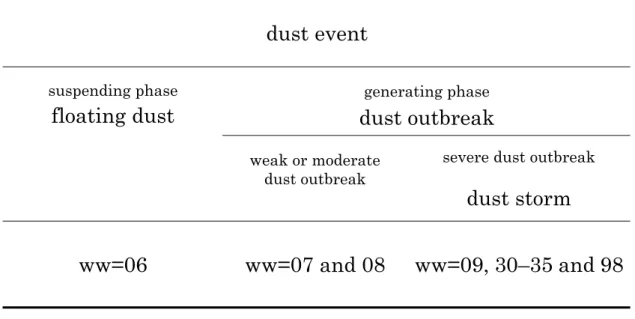
ww=06

ww=07 and 08

ww=09, 30–35 and 98

Table 2.2. Definitions about phenomena of aeolian dust. Symbolic letters “ww”

(41)

Legend of Land Cover Types in this study

Numbers of Global Ecosystems Legend (See Appendix 2)

Bare Desert ₀₈

Semi Desert ₁₁

Semi Desert Shrubs ₅₁

Grass/Shrub _{02, 07, 10, 16, 17, 40, 41, 42 and 87}

Cultivation _{30, 31, 35, ···, 39, 92, 93 and 94}

Savanna _{43, 58 and 91}

Forest 03, ···, 06, 18, ···, 29, 32, 33, 34, 48, 54, 56, 57, 60, 61, 78, 79 and 90

Tundra _{09, 53 and 63}

others _{others of the above}

Table 2.3. Legend of land cover types in this study (left column) and their

corresponding to numbers of the Global Ecosystem Legend (right column). The

(42)

27

(43)

Chapter 3 Potential Dust Sources

3.1 Geographical characteristics of East Asia

A conspicuous characteristic of East Asian geography is its massive topography. Figure 3.1 shows topography around the global dust belt shown by Prospero et al. [2002] (section 1.4.2) (a) and around East Asia (b). Topography affects atmospheric and land surface environments. As a result, three following geographical characteristics are essential for the aeolian dust outbreak in East Asia: (1) frequent synoptic disturbances in spring, (2) complicated distribution of land cover types, and (3) frequent snow covers in early spring. In this section, the relations among the aeolian dust outbreak, these three geographical characteristics and massive topography in East Asia are described.

3.1.1 Frequent synoptic disturbances in spring

It is well known that strong winds cause aeolian dust outbreaks when synoptic disturbances pass over the regions around the Gobi Desert (Fig. 3.2) [Watts, 1969; Pye, 1987; Littmann, 1991; Goudie and Middleton, 1992; Sun et al., 2001; Youlin, 2001; Gao et al, 2002; Qian et al., 2002]. These synoptic disturbances derive from Altai-Sayan lee cyclogeneses indicated by Chen et al. [1991]. Chen et al. [1991] show frequent cyclogeneses around the lee sides of the Altai-Sayan Mountains in spring (Fig. 3.3) and indicate that these cyclogenetic events occur by the effect of lee low.

(44)

29

Figure 3.4 is a SeaWiFS true color image of April 16, 1998, which shows yellow (or brown) cloud of aeolian dusts and white cloud due to a synoptic disturbance in the beginning stage of the trans-Pacific dust transport. Figure 3.5 shows surface meteorological sites where aeolian dusts were observed near the same time of the SeaWiFS image (03 UTC, April 16). The cloud image by GMS IR1 channel is illustrated in the same figure. According to Fig. 3.5, aeolian dusts near the land surface can be found in the back of a cold front. Uno et al. [2001] simulated this event and they indicated three-dimensional structures (Fig. 3.6) and time-height cross sections (Fig. 3.7) of these aeolian dusts. Aeolian dusts are horizontally and vertically transported by this synoptic disturbance (Fig. 3.6). As a result, aeolian dusts reach earlier in the higher level than in the lower level (Fig. 3.7). There are some regions where yellow aeolian dust clouds can be found in the SeaWiFS image (Fig. 3.4) but aeolian dusts were not observed at land surface (Fig. 3.5). Furthermore, there are other regions where white and yellow clouds are mixed in Fig. 3.4. It is practically certain that these indicate the transport of aeolian dusts into the upper level by this synoptic disturbance.

3.1.2 Complicated distribution of land cover types

Figure 3.8 shows the distribution of land cover types around the global dust belt (a) and around East Asia (b). Regions of each land cover type are distributed as an east-west belt in north part of Africa (Fig. 3.8a). East-west belts of Bare Desert, Semi

(45)

Shan Mountains, Altai Mountains. These topographies complicate the distribution of land cover types. Rodwell and Hoskins [1996], Sasaki [2002] and Sato and Kimura [2004] discussed why arid and semiarid regions distribute in relatively high latitude in East Asia with reference to the massive topography (see next section). These complicated distribution of land cover types suggest that aeolian dust sources also complicatedly distribute in East Asia.

3.1.3 Frequent snow covers in early spring

Regions of Bare Desert and Semi Desert Shrubs in East Asia and Central Asia are located in higher latitude in comparison with Africa and the Middle East (Fig. 3.8a). Therefore, snow frequently covers dust sources in East Asia and Central Asia in early spring (Fig. 3.9), and this snow cover condition largely affects aeolian dust outbreaks. Past studies have indicated that the topographies make arid conditions in East Asia and Central Asia. Rodwell and Hoskins [1996] explain the arid condition around the Aral Sea by their theory of monsoon-desert mechanism, which is that a diabatic heating in the Asian monsoon induces a decent flow around the Aral Sea. Sasaki [2002] obtains a result that the Altai-Sayan Mountains reduce inflow of water vapor into the Gobi Desert in spring and most of synoptic disturbances are not accompanied by precipitation in this season. According to Sato and Kimura [2004], the effect of heating by the Tibetan Plateau induces a descent flow above the Gobi Desert in summer. The

super arid condition in the Taklimakan Desert is induced by the obstruction of inflow of water vapor from the surrounding mountains.

3.2 Potential dust sources in the global dust belt

(46)

31

frequency corresponds to about 10 dust outbreaks for a month at a site where eight observations are conducted for a day (i.e., 3-hourly observation). A WMO synoptic observatory is considered to be a potential dust source when the maximum frequency is high. A potential source is assumed to be a site whose maximum frequency exceeds 2 %. Under this assumption, potential dust sources (i.e., open circles in Fig. 3.10a) are distributed more widely in comparison with dust source regions shown by previous studies (Figs. 1.3, 1.4, 1.6 and 1.7). For example, dust sources in Fig. 3.10a are distributed in tropical rain forests of the Indochina Peninsula, Indonesia and Africa, although these regions are not dust sources in previous studies. Rather than Fig. 3.10a, the distribution of potential dust sources in Fig. 3.10b fits dust sources shown by previous studies. From these results, we define a potential dust source as an observatory, whose maximum frequency exceeds 4 %. On the contrary, we define a non-dust-source as an observatory, whose maximum frequency does not reach 4 %. According to Fig. 3.10b, potential dust sources are distributed mainly in regions of Bare Desert, Semi Desert Shrubs, Grass/Shrub, Cultivation, and Savanna. These are distributed along the global dust belt indicated by Prospero et al. [2002]. Most of sites in regions of Bare Desert and Semi Desert Shrubs are potential dust sources. Many potential dust sources are found in regions of Grass/Shrub, Savanna and Cultivation, although most of sites are non-dust-sources in these regions. It cannot be judged whether Semi Desert regions, which are distributed in high lands as the Tibetan

Plateau and the Ethiopian Plateau, possess potential of dust source or not, because there are a small number of sites in this land cover type.

3.3 Potential dust sources in East Asia

(47)

(48)

33

(49)

(50)

35

(51)

(52)

37

(53)

(54)

39

(55)

(56)

41

(57)

Fig. 3.10. Distributions of potential dust sources around the global dust belt

(58)

43

(59)

Chapter 4 Characteristics of Aeolian Dust in East Asia

It has been well known that East Asia possesses two major dust source regions; one

is the Gobi Desert and the other is the Taklimakan Desert. Although these two dust

sources adjoin, different weather systems cause aeolian dust outbreaks. As described in

section 3.1, when a synoptic disturbance passes over the Gobi Desert, strong winds

accompanied by this disturbance cause dust outbreaks. On the other hand, most of

synoptic disturbances cannot directly pass over the Taklimakan Desert because this

desert is surrounded by steep topography such as the Tian Shan Mountains, the Pamirs

and the Kunlun Mountains. According to Sun et al. [2001], dust outbreaks occur by

easterly cold airflows in a branch of a major route of synoptic disturbance (Fig. 3.2).

Aoki [2003] indicates that there are three major routes of synoptic disturbance causing

dust outbreaks: they are easterly cold airflow same as Sun et al. [2001], northerly one

beyond the Tian Shan Mountains, and westerly one beyond the Pamirs.

Referring to the above, we provide two analysis regions in this chapter: one is the

region “around the Gobi Desert” (Region I) and the other is “the Taklimakan Desert”

(Region II) (Fig. 4.1). The region around the Gobi Desert includes potential dust sources

in regions of Grass/Shrub, Cultivation and Savanna surrounding the Gobi Desert

(section 3.3). In this chapter, characteristics of aeolian dust in Regions I and II are

studied in sections 4.1 and 4.2, respectively. Aeolian dusts in these two regions are

(60)

45

4.1 Aeolian dust around the Gobi Desert

4.1.1 Introduction

The long-term variations of dust event frequencies have exhibited a negative trend

over the last 40 years in China [Qian et al., 2002; Parungo et al., 1994; Sun et al., 2000;

Yoshino, 2002]. However, East Asian dust events have become uncommonly active in

recent years. A report for the press of Japan Meteorological Agency

(http://www.jma.go.jp/JMA_HP/jma/press/0204/15a/kosa.pdf) stated that it is

remarkable that Kosa (i.e., yellow sand) events were frequently observed in Japan in

the last three years (2000 – 2002) (Fig. 4.2). Dust phenomena also frequently occurred

after 2000 in Korea. Dust phenomena were observed over 10 days in Seoul City in every

year after 2000, although the average number of days of dust phenomena was 5.2 from

1915 – 2002 [Chun et al., 2002; Chun et al., 2001]. In addition, large-scale dust events

that transported mineral dust particles across the Pacific Ocean occurred in 1998 and

2001 [e.g., Husar et al., 2001]. The reasons for the recent trend of active dust events and

any relation to the dust outbreaks in East Asia have not been clarified.

Aeolian dust is usually generated by strong surface wind on arid and/or semi-arid

regions with low vegetation cover. East Asian cyclone activity is strong around the Gobi

Desert in spring [Chen et al., 1991], and the Gobi Desert is a major dust source region in

East Asia.

The relationship between dust outbreaks and strong winds was investigated in

section 4.1 to clarify the recent active dust events around the Gobi Desert. We conducted

statistical analyses of dust outbreaks and strong surface winds around the Gobi Desert

during the past ten years (1993 – 2002), using the present weather code and the surface

wind velocity obtained from the SYNOP report [WMO, 1974].

4.1.2 Data and methods

The data used in section 4.1 were the present weather code and surface wind velocity

(61)

from SYNOP reports. The analysis period was from January 1993 to June 2002. The

code numbers of the_{present weather, ww=07, 08, 09, 30-35, and 98, were classified as}

the dust outbreaks as defined in section 2.1.2. A strong surface wind was defined as one

with a velocity exceeding 6.5 m/s, which is the threshold for a dust outbreak in many

numerical models (see section 2.1.3). Threshold velocities actually exhibit various

values with differing land surface conditions. However, a constant value was used to

define a strong wind in this study, because land surface conditions and the threshold

velocity for each land surface condition have not yet been clarified.

As defined in section 2.1.4, the dust outbreak frequency is the percentage of the

number of dust outbreaks to the total number of observations within a given period at

each observatory and/or given region. Similarly, the strong wind frequency is the

percentage of the number of strong winds to the total number of observations.

4.1.3 Analysis region

Figure 4.3 illustrates the maximum monthly dust outbreak frequency (hereafter,

maximum frequency) from January 1993 to June 2002 at each observatory. As defined

in section 3.2, a site is a potential dust source during this period when the maximum

frequency exceeds 4 % at such a site. We represent the analysis region in section 4.1 by

a box in Fig. 4.3 (33.5°N – 52.0°N, 88.5°E – 131.5°E); this box indicates the north, east,

and south boundaries of the potential dust source region around the Gobi Desert. Thus,

a total of 105 potential dust source observatories are included within the analysis region.

The data at these observatories were used in the statistical analyses in sections 4.1.4.1,

4.1.4.2, and 4.1.4.3.

4.1.4 Results

4.1.4.1 Seasonal variations

The white bar chart and line graph with white circles in Fig. 4.4 indicate the

frequencies of monthly dust outbreaks and strong winds from January 1993 to June

(62)

47

studies [Littmann, 1991; Parungo et al., 1994]. Two-thirds of the dust outbreaks can be

observed in March, April, and May. In contrast, dust outbreaks are the least frequent in

summer (July, August, and September). Strong winds also occur most frequently in

spring and least frequently in summer. A weak secondary peak of strong wind frequency

occurs around November; however, the dust outbreak frequency has no peak in this

season.

4.1.4.2 Year-to-year variation

The dust outbreak frequency in spring has been greater in the last three years (2000

– 2002) than in the preceding seven years (1993 – 1999) (Fig. 4.5). The last three years

(2000 – 2002) will hereafter be referred to as the dust-frequent years (DFY), and the

previous seven years (1993 – 1999) as the dust-normal years (DNY). The year-to-year

variation of Kosa events (Fig. 4.2) is similar to that of dust outbreaks in East Asia (Fig.

4.5); i.e., Kosa is frequently observed in DFY. The strong wind frequency is also high in

DFY and low in DNY.

A clear positive correlation was found between dust outbreak frequencies and strong

wind frequencies in year-to-year variations. However, the month of April was an

exception in both 1995 and 1998. The strong wind frequency was as high as in DFY in

1995; nevertheless, the dust outbreak frequency was almost equal to the average of the

DNY. In contrast, the dust outbreak frequency was somewhat high in 1998, although

the strong wind frequency was almost equal to the average of the DNY. The dust

phenomena in exceptional years will be discussed in section 6.3.1.

4.1.4.3 Months that dust outbreaks increased

The black bar chart and line graph with black dots in Fig. 4.4 indicate the

frequencies of monthly dust outbreaks and strong winds for DFY (2000 – 2002).

Although the most frequent months for dust outbreaks are March, April, and May in a

10-year average (white bar chart), remarkable increases of dust outbreak frequencies

occurred in March and April, while no increase was observed in May. The strong wind

(63)

March and April.

4.1.4.4 Spatial distribution of dust outbreaks

Figures 4.6 (a) and (b) illustrate the spatial distribution of the dust outbreak

frequencies for March and April in DNY (1993 – 1999) and DFY (2000 – 2002). Areas of

frequent dust outbreaks can be seen in the western part of the analysis region in DNY

(Fig. 4.6a), i.e., around southern Mongolia (about 44°N, 105°E), the Badain Jaran

Desert (about 42°N, 102°E), and the western Loess Plateau (about 40°N, 105°E). The

dust outbreak frequencies were low at most observatories in the eastern part of the

analysis region, i.e., around the North China Plain (about 40°N, 115°E), northeastern

China (about 45°N, 125°E), and the Korean Peninsula (about 38°N, 127°E). In contrast,

the region of frequent dust outbreaks expanded to the east in DFY (Fig. 4.6b), and dust

outbreaks frequently occurred at many observatories in the eastern region. Although

the area of frequent dust outbreaks expanded little into the western region, dust

outbreak frequency increased at each observatory.

4.1.4.5 Spatial difference in dust outbreaks with strong winds

Section 4.1.4.2 described the correlation between dust outbreaks and strong winds in

the year-to-year variations; the spatial differences in dust outbreaks with strong winds

are shown in Fig. 4.7. This figure is a scatter diagram of increases in the frequency of

strong winds (abscissa) and dust outbreaks (ordinate) from DNY (1993 – 1999) to DFY

(2000 – 2002). The frequencies were calculated for the period from March to April at

each observatory. Each symbol in this figure indicates the dust outbreak frequency in

DFY.

Most of the plots are in the first quadrant. This indicates that the dust outbreak

frequencies increased at observatories where the strong wind frequencies increased.

Dust outbreak frequencies increased remarkably at sites of frequent dust outbreaks

(black circle plots). This signifies that an increase of strong winds is always

accompanied by an increase of dust outbreaks in these regions. No dust outbreaks were