つくばリポジトリ JI 12 P12009

(1)

(2)

Journal of Instrumentation

OPEN ACCESS

Study of the material of the ATLAS inner detector

for Run 2 of the LHC

To cite this article: M. Aaboud et al₂₀₁₇JINST12_P12009

View the article online for updates and enhancements.

-2017 JINST 12 P12009

Published by IOP Publishing for Sissa Medialab

Received:July 11, 2017

Accepted:October 27, 2017

Published:December 7, 2017

Study of the material of the ATLAS inner detector for Run

2 of the LHC

The ATLAS collaboration

E-mail: [email protected]

Abstract:The ATLAS inner detector comprises three diﬀerent sub-detectors: the pixel detector, the silicon strip tracker, and the transition-radiation drift-tube tracker. The InsertableB-Layer, a new innermost pixel layer, was installed during the shutdown period in 2014, together with modiﬁcations to the layout of the cables and support structures of the existing pixel detector. The material in the inner detector is studied with several methods, using a low-luminosity√s = 13TeV pp collision

sample corresponding to around 2.0nb−1 collected in 2015 with the ATLAS experiment at the LHC. In this paper, the material within the innermost barrel region is studied using reconstructed hadronic interaction and photon conversion vertices. For the forward rapidity region, the material is probed by a measurement of the eﬃciency with which single tracks reconstructed from pixel detector hits alone can be extended with hits on the track in the strip layers. The results of these studies have been taken into account in an improved description of the material in the ATLAS inner detector simulation, resulting in a reduction in the uncertainties associated with the charged-particle reconstruction eﬃciency determined from simulation.

Keywords: Detector modelling and simulations I (interaction of radiation with matter, interac-tion of photons with matter, interacinterac-tion of hadrons with matter, etc); Particle tracking detectors; Performance of High Energy Physics Detectors

(4)

2017 JINST 12 P12009

Contents

1 Introduction 1

2 ATLAS detector 3

3 Data and simulation samples 5

3.1 Data sample 5

3.2 Monte Carlo simulation 5

3.3 Simulated descriptions of the inner detector 6

4 Overview of analysis methods 6

4.1 Reconstruction of hadronic interaction and photon conversion vertices 7

4.2 Track-extension eﬃciency 8

4.3 Track impact parameter resolution 9

5 Reconstruction and data selection 11

5.1 Track reconstruction 11

5.2 Vertex reconstruction 11

5.3 Data selection 12

5.3.1 Hadronic interactions 12

5.3.2 Photon conversions 13

5.3.3 Track-extension eﬃciency 13

5.3.4 Transverse impact parameter resolution 15

6 Characterisation of material in data and MC simulation 15

6.1 Radial and pseudorapidity regions 15

6.2 Radial position oﬀset 15

6.3 Beam pipe 15

6.4 IBL and its support tubes 18

6.5 Outer barrel layers 19

6.6 Regions between pixel and SCT detectors 19

7 Measurement of material in data and MC simulation 19

7.1 Hadronic interactions 19

7.1.1 Corrections 22

7.1.2 Description of systematic uncertainty estimation 23

7.2 Photon conversions 26

7.2.1 Corrections 28

7.2.2 Systematic uncertainties 28

7.3 Track-extension eﬃciency 29

(5)

2017 JINST 12 P12009

8 Results and discussion 33

8.1 Transverse impact parameter resolution 33

9 Conclusion 39

The ATLAS collaboration 43

1 Introduction

Data recorded by tracking detectors are used to reconstruct the trajectories of charged particles and determine their momenta. The location of particle interactions with the material of the detector can be identified by reconstructing interaction vertices. Obtaining an accurate description of this mate-rial is essential to understand the performance of the detector. For the ATLAS detector [1], nuclear interactions ofprimary particleswith the material are the largest source of secondary particles;1 hence the uncertainty in the track reconstruction efficiency is directly coupled to the accuracy of knowing the amount and type of material [2,3]. For electromagnetic calorimeters, the knowledge of the material situated between the collision point and the calorimeter is essential to calibrate the energy of reconstructed electrons, unconverted and converted photons [4]. The precision of track reconstruction parameters is also sensitive to the amount of material of the tracking detector. The precise knowledge of it is important for the performance of the reconstruction of the high-level objects based on track reconstruction like identification of b-hadrons (b-tagging). Furthermore, searches for new physics performed by reconstructing the decay vertex of long-lived particles require a precise description of the material to define fiducial decay volumes with minimal back-ground [5]. The accuracy of the description of the material structure is thus an essential foundation for physics analysis with the ATLAS detector. In fact, it plays a central role together with other key ingredients required for particle reconstruction, e.g. the magnetic field description, understanding of the processes occurring inside semiconductor sensors or gases, and the alignment of the components. The description of the material including the geometrical layout and atomic composition, hereafter referred to as thegeometry model, is based on engineering design drawings of the detector,

together with supporting measurements of the masses, dimensions and compositions of detector components. During construction of the ATLAS inner detector (ID) [1], detailed measurements of the mass of detector components were undertaken, and the corresponding masses in the geometry model were adapted to agree with the measurement as accurately as possible [1]. The amount of material in the Run 12as-built ID [1] is generally known to an accuracy of about 4–5%. However, obtaining a satisfactory geometry model is challenging because of the complexity of the detector design and the need to thoroughly validate the description.

Several in situmethods using collision data have been developed to estimate the amount of

material within the tracking detectors of high-energy physics experiments [2,6,7]. Reconstructing

1In this paper,primary particlesrefer to particles which are promptly produced in theppcollision, whilesecondary particlesrefer to those which are produced in the decays of primary particles or through their interaction with material.

(6)

2017 JINST 12 P12009

photon conversion vertices is a traditional method to measure the material of tracking detectors [8],

taking advantage of precise theoretical understanding of electromagnetic interaction processes. The reconstruction of hadronic interaction vertices instead of photon conversions is a complementary approach [9,10] — it is sensitive to the material through nuclear interactions, and oﬀers much better resolution in the radial position of the vertex compared to the case of photon conversion. However, the description of hadronic interactions is complex and only phenomenologically modelled in the simulation. Another complementary approach which is applicable to the all tracking acceptance is to measure the nuclear interaction rate of charged hadrons through hadronic interactions, referred to as thetrack-extension eﬃciencymethod. The precision of each measurement varies depending

on the detector region. All of these approaches are used together to measure a large part of the inner detector’s volume and cross-check individual measurements. Using the hadronic interaction approach, ATLAS has performed measurements of the inner detector’s material in Run 1 of the LHC [9,10]. The measurements were performed by comparing observables sensitive to the material in data and Monte Carlo (MC) simulation.

The ATLAS inner detector system is immersed in a 2 Taxial magnetic ﬁeld, and provides measurements for charged-particle trajectory reconstruction with full coverage in φ in the range |η_| <2.5.₃ It consists of a silicon pixel detector (pixel), a silicon micro-strip detector (SCT) and a transition-radiation straw-tube tracker (TRT). During the LHC shutdown period in 2013–2014, be-tween Run 1 and Run 2, the inner detector was upgraded with the installation of a new pixel-detector layer together with a new, thinner beam pipe, referred to as the insertableB-layer (IBL) [11]. In addition, the pixel detector was extracted and renovated. This involved replacement of pixel service panels (cables, cooling pipes and support structures) located in the forwardηregion of the pixel

de-tector. These changes motivated the material re-evaluation and creation of a new ID geometry model. The characteristics of a material in terms of interaction with high-energy particles are quantiﬁed by the radiation length, X0, and nuclear interaction length, λI. In this paper, the unit of mm is used to quantify these properties.4 The radiation length X0 is the mean path length over which a high-energy (E ≫ 2me) electron loses all but1/e of its energy due to bremsstrahlung. Similarly, λ_I is the mean path length to reduce the ﬂux of relativistic primary hadrons to a fraction 1_/e. The

amount of material associated with electromagnetic interactions along a particular trajectoryCis represented by a dimensionless number N_X[C₀], frequently referred to as the number of radiation lengthsin the literature.5 This is calculated as a line integral:

N_X[C]

0 =

∫

C

ds 1 X0(s),

where X0(s) is the local radiation length of the material at the position s along the trajectory C. Similarly, the amount of material associated with nuclear interactions is represented by a

3ATLAS uses a right-handed coordinate system with its origin at the nominal interaction point (IP) in the centre of the detector and thez-axis along the beam pipe. Thex-axis points from the IP to the centre of the LHC ring, and they-axis points upwards. Cylindrical coordinates(r, φ)are used in the transverse plane,φbeing the azimuthal angle around the

z-axis. The pseudorapidity is deﬁned in terms of the polar angleθasη=−ln tan(θ/2). Angular distance is measured in units of∆R≡p(∆η)2+(∆φ)2.

4There is another common convention of using g/cm2in the literature [12].

(7)

2017 JINST 12 P12009

dimensionless number denoted byN_λ[C]

I :

N_λ[C]

I =

∫

C

ds 1

λI(s) .

This paper presents studies of the ATLAS Run 2 ID material using hadronic interactions, photon conversions and the track-extension eﬃciency measurement. An additional study of the transverse impact parameter resolution of tracks is also presented. The paper is organised as follows. Section2

provides an overview of the ATLAS detector and further details of the inner detector. Data and MC simulation samples together with the various geometry model versions used in this paper are introduced in section3. The methodology of the measurements presented in this paper is described in section 4. Event reconstruction and data selection are presented in section 5. A qualitative overview of the comparison of data to MC simulation is discussed in section6. Analysis methods and systematic uncertainties of each of the individual measurements are described in section7. The results of the measurements are presented and discussed in section8. Finally, conclusions of this work are presented in section9.

2 ATLAS detector

The ATLAS detector at the LHC [1] covers nearly the entire solid angle around the collision point. It consists of an inner detector (ID) surrounded by a thin superconducting solenoid, electromagnetic and hadronic calorimeters and a muon spectrometer incorporating three large superconducting toroidal magnet systems. Only the inner detector and trigger system are used for the measurements presented in this paper.

The pixel detector (including the IBL) spans the radial region (measured from the interaction point) of 33–150 mm, while the SCT and TRT detectors span the radial regions 299–560 mm and 563–1066 mm, respectively. The ID is designed such that its material content has a minimal eﬀect on the particles traversing its volume. Figure1shows the layout of the ID in Run 2.

The innermost pixel layer, the IBL, consists of 14 staves which cover the region|η_| <3.03 with

over 12 million silicon pixels with a typical size of 50µm₍r-φ_)×250µm₍z₎each [11]. The addition of the IBL improves the track reconstruction performance; for example, both the transverse and lon-gitudinal impact parameter resolution improve by more than 40% in the best case of tracks with trans-verse momentum (pT) around 0.5 GeV [13]. Here, the transverse impact parameter,d0, is deﬁned as the shortest distance between a track and the beam line in the transverse plane. The longitudinal impact parameter,z0, is deﬁned as the distance inzbetween the primary vertex and the point on the track used to evaluated0. The average amount of material introduced by the IBL staves corresponds to approximately NX0 = 1.5%, for particles produced perpendicular to the beam line, originating

fromr =0. The IBL staves are placed between the inner positioning tube (IPT) atr =29.0 mm and

the inner support tube (IST) atr =42.5 mm. The IPT and IST are made from carbon ﬁbre and resin.

The thickness of the IPT varies from 0.325 mm at_|z| <311 mm, to 0.455 mm at the outermost edge.

(8)

2017 JINST 12 P12009

Figure 1. Ther-zcross-section view of the layout of a quadrant of the ATLAS inner detector for Run 2.

The top panel shows the whole inner detector, whereas the bottom-left panel shows a magniﬁed view of the pixel detector region. Compared to Run 1, the IBL (shown in red in the bottom-left panel) and its services, together with the new beam pipe, were added.

with polyimide tapes and aerogel thermal insulators. There is no thermal insulator in the central part of the new beam pipe at _|z| < 311mm, in order to reduce material thickness. The material composition of the new beam pipe was measured using X-rays as well as by mass measurements to a precision of 1% before installation.

(9)

2017 JINST 12 P12009

module is composed of two layers of silicon micro-strip detector sensors glued back to back with a

relative stereo angle of40mrad. The SCT barrel layers are enclosed by the inner and outer thermal enclosures, referred to as the SCT-ITE and SCT-OTE respectively, which are located atr _≃255 mm andr ≃ 550 mm. The TRT is the outermost of the ID sub-detectors and consists of more than 350 000 gas-ﬁlled straw tubes. The structures of the SCT and TRT are unchanged since Run 1.

The ATLAS trigger system consists of a level-1 hardware stage and a high-level trigger software stage [14]. The level-1 decision used in the measurements presented in this paper are provided by the minimum-bias trigger scintillators (MBTS), which were replaced between Run 1 and Run 2. The MBTS are mounted at each end of the detector in front of the liquid-argon end-cap calorimeter cryostats at z = ±3.56 m and segmented into two rings in pseudorapidity (2.07 < |η| < 2.76 and

2.76 < _|η_| < 3.86). The inner ring is segmented into eight azimuthal sectors while the outer ring

is segmented into four azimuthal sectors, giving a total of twelve sectors per side.

3 Data and simulation samples

3.1 Data sample

Theppcollision data sample used to perform the measurements described in this paper was collected in June 2015 at a centre-of-mass energy of√s =13 TeV by the ATLAS detector at the LHC. During

this running period, the LHC was operating in a special conﬁguration with a low instantaneous luminosity. The average number of collisions per bunch crossing was approximately 0.005. The data were collected with triggers which required one or more counters above threshold on either side of the MBTS detectors. Events are retained for analysis if they were collected under stable LHC beam conditions and the detector components were operating normally. Approximately 130 million events passing the trigger condition are used in this study, corresponding to an integrated luminosity of around 2.0 nb−1.

3.2 Monte Carlo simulation

The Pythia 8 [15] (version 8.185), and Epos [16] (version LHCv3400) MC event generators are used to simulate minimum-bias inelastic ppcollisions. ThePythia 8model of inclusive pp interactions splits the total inelastic cross-section into non-diffractive (ND) processes, dominated byt-channel gluon exchange, and diffractive processes involving a colour-singlet exchange. TheA2 set of tuned parameters forPythia 8[17] was used in conjunction with theMSTW2008loparton distribution functions [18]. These samples were produced for the ND component, since there is little contribution from the diffractive components after full selection. Epos models inclusive ppinteractions with a parton-based Gribov-Regge [19] theory, which is an effective field theory inspired by quantum chromodynamics describing hard and soft scattering simultaneously. The LHCset of tuned parameters [20] of theEposMC event generator was used. BothPythia 8and Epos, tuned and set up as described above, are found to provide reasonable descriptions of the charged-particle multiplicity distributions measured inppcollisions at√s=13 TeV [21].

The modelling of the interactions of particles with material in theGeant4simulation [22], is referred to as aphysics list. The analysis presented in this paper uses theFTFP_BERTphysics list.

(10)

2017 JINST 12 P12009

energy larger than 4 GeV, and the Bertini-style cascade for hadrons below 5 GeV [25]. In the

energy region where these two models overlap, one model is randomly selected to simulate a given interaction, with a probability weight which changes linearly as a function of kinetic energy.

3.3 Simulated descriptions of the inner detector

Simulatedppcollision events generated byPythia 8andEposwere processed through the ATLAS detector simulation [26], based onGeant4, and are reconstructed by the same software as used to process the data. The ATLAS detector is described withinGeant4by a collection of geometry models, each describing the sub-detectors that constitute the full detector. The geometry model for the inner detector describes both the active elements of the detectors (e.g. the silicon pixel sensors) and the passive material (e.g. support structures and cables). The measurements presented in this paper make use of several alternative ID geometry models, summarised below:

Original — This ID geometry model represents the nominal geometry model used to generate

MC simulation samples produced in 2015. The studies presented in this paper identiﬁed a number of missing components in the simulated description of the IBL.

Updated— A modiﬁed version of theoriginalgeometry model which was created for this study. In

this model, several additional components are added to the simulated description of the IBL reflecting the observations which are described in section6. These additional components include flex buses and a number of surface-mounted devices on the front-end of the modules. Small modifications to the positioning of each IBL stave and the material densities of the IBL support structures were also made.

Figures 2 and3 show respectively the radial and z-distributions of the number of radiation lengths for both theoriginalandupdated geometry models. For the updated geometry, ﬁgure4

shows the distribution of the number of radiation lengths in ther-zview, and ﬁgure5showsNλ_I as

a function ofη.

Based on theoriginalandupdatedgeometry models, collections ofdistortedgeometry models

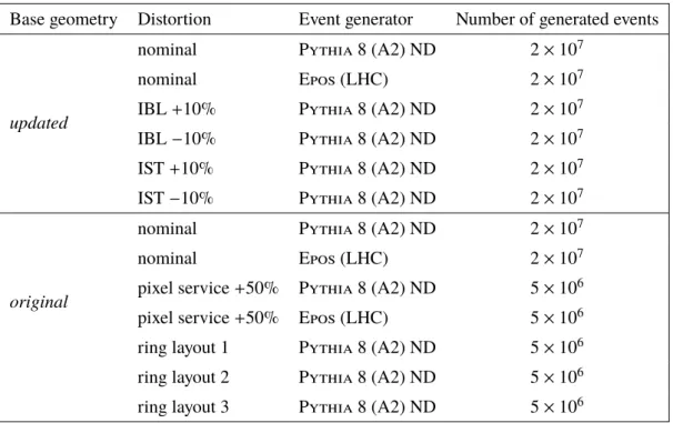
were created, in which the density of a variety of components is artificially scaled by a known amount. Furthermore, three modified geometry models were created in which a ring of passive material was added to the original geometry model. The rings were positioned at differentr-z coordinates and orientations in the region between the pixel and SCT detectors. This was done in order to test the sensitivity of the track-extension efficiency method to the material location. These distorted models are used to calibrate the material measurement methods and assess the systematic uncertainties associated with the measurements. Table1summarises the collection of MC samples used in this paper. Pythia 8is used as the nominal event generator for all of the studies except for the hadronic interaction study, which usesEposas the nominal event generator since it is found to provide a better description of events with decays in flight thanPythia 8.

4 Overview of analysis methods

(11)

2017 JINST 12 P12009

Table 1.List of MC samples used in the analyses, with the base geometry model, presence of an additional

distortion, the event generator used and the number of generated events.

Base geometry Distortion Event generator Number of generated events

updated

nominal Pythia 8(A2) ND 2_×107

nominal Epos(LHC) 2_×107

IBL₊10% Pythia 8(A2) ND 2_×107 IBL₋10% Pythia 8(A2) ND 2_×107 IST+10% Pythia 8(A2) ND 2_×107 IST₋10% Pythia 8(A2) ND 2_×107

original

nominal Pythia 8(A2) ND 2_×107

nominal Epos(LHC) 2_×107

pixel service+50% Pythia 8(A2) ND 5×106

pixel service+50% Epos(LHC) 5×106

ring layout 1 Pythia 8(A2) ND 5_×106

4.1 Reconstruction of hadronic interaction and photon conversion vertices

The hadronic interaction and photon conversion analyses aim to identify and reconstruct the in-teraction vertices of hadronic inin-teractions and photon conversions to probe the accuracy of the ID material content within the detector simulation. Vertices corresponding toppinteraction positions are referred to asprimary vertices, while other vertices corresponding to in-ﬂight decays, photon

conversions and hadronic interactions are collectively referred to assecondary vertices. In this

pa-per, only secondary vertices with a distance from the beam line of more than 10 mm are considered. The properties of hadronic-interaction and photon-conversion candidates are compared between the data and the MC simulation.

Photon conversions are well-understood electromagnetic processes which exhibit a high recon-struction purity. The vertex radial position resolution is around 2 mm, limited by the collinearity of the electron-positron pair. In contrast, hadronic interactions are complex phenomena which are diﬃcult to model in simulation. Their reconstruction suﬀers from backgrounds associated with hadron decays and combinatoric fake vertices. However, the radial position resolution is far better than for photon conversions. Resolutions ofO(0.1₎mmcan be achieved due to large opening angles between the daughter particles. This facilitates a detailed radiography of the material, including minute components, e.g. the capacitors mounted on the surfaces of the pixel modules, allowing their location to be determined precisely.

(12)

2017 JINST 12 P12009

r [mm]

0 100 200 300 400 500 600

/ mm]

3

−

10

×

r [

∆

/ ₀

X

N

∆

0 1 2 3 4 5 6 7

Original Geometry

Updated Geometry Simulation

|z| < 300 mm

ATLAS

BP IBL PIX1 PIX2 PIX3

PSF

PST SCT-ITE SCT1 SCT2 SCT3 SCT4 SCT-OTE

(a)r<600 mm.

r [mm]

20 25 30 35 40 45 50 55 60 65 70 75

/ mm]

3

−

10

×

r [

∆

/ 0

X

N

∆

0 1 2 3 4 5 6 7 8 9

Simulation |z| < 300 mm

ATLAS Original Geometry

Updated Geometry

BP IPT IBL IST PIX1

(b)20 mm<r <75 mm.

Figure 2. The diﬀerential number of radiation lengths as a function of the radius,∆NX0/∆r, averaged over

|z_|<300 mm(a)forr<600 mmand(b)for20 mm<r<75 mmfor theoriginalgeometry and theupdated geometry. The simulated material is sampled for eachz-position along a straight radial path (perpendicular

to the beam line).

of the SCT atr ≃300 mm, and are suitable for probing the barrel structures including the IBL and the new beam pipe. Further details can be found in section7.

4.2 Track-extension efficiency

In an attempt to have as few particle interactions with material as possible, most of the pixel services, which reside between the pixel and SCT detectors, are located together in the forward region (approximately1.0 < _|η_| < 2.5). This region of the inner detector is more challenging to model within the simulation than the central barrel region, due to the complexity of the structure and the amount of material, as shown in ﬁgures4and5.

(13)

2017 JINST 12 P12009

z [mm]

400

− −300 −200 −100 0 100 200 300 400

[%]0 X N 0 0.1 0.2 0.3 0.4 0.5 0.6 0.7 0.8

0.9 Original Geometry ATLAS

Updated Geometry Simulation 22 < r < 27 mm

(a)Beam Pipe.

z [mm] 400

− −300 −200 −100 0 100 200 300 400

[%]0 X N 0 0.2 0.4 0.6 0.8 1 ATLAS Original Geometry

(b)IPT.

z [mm] 400

− −300 −200 −100 0 100 200 300 400

[%]0 X N 0 0.5 1 1.5 2 2.5 3 3.5 4 4.5 ATLAS Original Geometry

(c)IBL.

z [mm] 400

− −300 −200 −100 0 100 200 300 400

[%]0 X N 0 0.2 0.4 0.6 0.8

1 Original Geometry_{Updated Geometry} ATLAS_Simulation 40 < r < 45 mm

(d)IST.

Figure 3. Number of radiation lengths as a function of thez-coordinate for diﬀerent radial sections for the

originalgeometry and theupdatedgeometry.

hereafter). Hits in the SCT and TRT detectors associated with the secondary particles produced in the hadronic interaction are unlikely to be associated to the tracklet. The rate of hadronic interactions can be related to the so-calledtrack-extension eﬃciency, denoted by_Eextand deﬁned as:

Eext ≡

nmatched_tracklet

ntracklet ,

wherentrackletis the number of tracklets satisfying a given set of selection criteria andnmatched_tracklet is the number of those tracklets that are matched to a combined track. The efficiency_Eextis related to the amount of material crossed by a particle and is therefore dependent on the kinematics and origin of the particle. For particles with sufficiently high pT , when averaging overφand restricting the z-position of the primary vertex (zvtx) to a sufficiently narrow range, the particle trajectoryCcan be approximately described as a function ofηalone.

4.3 Track impact parameter resolution

The resolution of the track transverse impact parameter d0, denoted σd0, depends on the track

momentum. The resolution in the high-pT limit is largely determined by the intrinsic position resolution of detector sensors and the accuracy of the alignment of each detector component. At suﬃciently low pT, the eﬀects of multiple scattering dominate the resolution. At low pT, σd0 is

sensitive to the amount of the material in the ID, particularly that closest to the collision point. By measuring σd0, it is possible to cross-check the accuracy of the geometry model using an

(14)

2017 JINST 12 P12009

Figure 4. Ther-zdistribution of the diﬀerential number of radiation lengths, ∆NX0/∆r, for the updated geometry model of a quadrant of the inner detector barrel region of the pixel detector and the SCT. The simulated material is sampled for eachz-position along a straight radial path (perpendicular to the beam line).

η

0 0.5 1 1.5 2 2.5

I

λ

N

0.00 0.05 0.10 0.15 0.20 0.25 0.30 0.35 0.40

150 mm < r < 250 mm 45 mm < r < 150 mm 27 mm < r < 45 mm r < 27 mm

Simulation

ATLAS

Figure 5. The amount of material associated with nuclear interactions,NλI =

∫

dsλ−_I1, averaged overφ, as

a function ofηin the positiveηrange integrated up tor ₌250 mm for theupdatedgeometry model. The simulated material is sampled fromz₌0 along a straight path with ﬁxedφ. The material within the inner

detector is shown separately for the regionsr <27 mm, 27 mm<r <45 mm, 45 mm<r <150 mm and

150 mm<r <250 mm, corresponding approximately to the beam pipe, IBL, pixel barrel and pixel service

(15)

2017 JINST 12 P12009

5 Reconstruction and data selection

5.1 Track reconstruction

Charged-particle tracks are reconstructed with a special conﬁguration (for low-luminosity running) of the ATLAS track reconstruction algorithm [27] optimised for Run 2 [28] down topTof100MeV.

Theinside-outtracking refers to the track reconstruction algorithm seeded from pixel and SCT hits

and extended to the TRT. In this algorithm, candidates are rejected from the set of reconstructed tracks if the absolute value of the transverse (longitudinal) impact parameter, d0 (z0) is greater than 10mm(250mm). Tracks originating from in-flight decay vertices (e.g.K_S0decays) inside the inner detector’s volume or from photon conversions may not have a sufficient number of pixel and SCT hits to satisfy the inside-out track finding. A second tracking algorithm, referred to as the

outside-inapproach, complements this by ﬁnding track seeds in the TRT and extending them back to

match hits in the pixels and SCT which are not already associated with tracks reconstructed with the inside-out approach. Nod0andz0requirements are applied for the outside-in tracking. Tracklets are reconstructed using the inside-out approach down topT of50MeV. Not all tracks reconstructed in the ID correspond directly to a charged particle traversing the detector. Coincidental arrangements of unrelated hits can give rise to so-calledfaketracks. Fake tracks (and similarly fake tracklets)

are identiﬁed in the MC simulation as those with a small fraction of hits originating from a single simulated charged particle [29].

5.2 Vertex reconstruction

Theprimaryvertices, i.e. positions of the inelastic proton-proton interactions, are reconstructed by

theiterative vertex ﬁndingalgorithm [30]. At least two charged-particle tracks withpTgreater than

100MeV are required to form a primary vertex. Thehard-scatterprimary vertex is deﬁned as the

primary vertex with the highest sum of thep_T2of the associated tracks. Other primary vertices are referred to aspile-upvertices.

Secondary vertices are reconstructed by the inclusive secondary-vertex ﬁnding algorithm,

which is designed to ﬁnd vertices from a predeﬁned set of input tracks within an event [9].

The configuration of the secondary-vertex reconstruction differs between the hadronic-interaction and photon-conversion analyses, reflecting the different topologies associated with the interactions. These differences are summarised in table 2. For hadronic interactions, tracks are required to have at least one SCT hit, _|d0| > 5 mm, a track-fitting χ2 divided by the number of degrees of freedom (Ndof) less than 5, and satisfy certain quality criteria. The requirement ond0 is imposed in order to efficiently reject combinatorial fake vertices. The fitted vertex must have a vertex-fitting χ2_/Ndofof less than 10. In addition, a geometrical compatibility criterion is applied. The tracks associated with the reconstructed vertex are required to have no hits in any detector layer inside thevertex radius, defined as the distance of the vertex in thex-yplane from the origin of the

ATLAS coordinate system, and are required to have hits in the closest outer layer beyond the vertex radius.

(16)

2017 JINST 12 P12009

two tracks, are selected. The vertices of the track pairs are ﬁtted while constraining the opening

angle between the two tracks (in both the transverse and longitudinal planes) at the vertex to be zero. Finally, only vertices built from two tracks, both of which are associated with silicon detector hits, are retained for further analysis.

In MC simulation, the truth matching of the secondary vertices is deﬁned as follows, using “truth” information from the generator-level event record. If the vertex has any fake tracks, it is clas-siﬁed as afakevertex. If all of the truth particles linked from the reconstructed tracks originate from

a single truth vertex, the reconstructed vertex is classiﬁed astruth-matched. Otherwise the vertex is

classified as fake. In the case of a truth-matched vertex, it is further classified intoin-flight decay,

photon conversionorinelasticvertex. A truth vertex is labelled as a photon conversion if the truth

particle identifier of the parent particle of the vertex is a photon. A truth vertex is labelled as an in-flight decay if the difference between the energy sum of outgoing truth particles and incoming parti-cle is less than 100 MeV. If the incoming partiparti-cle is a hadron and it is not labelled as an in-flight decay, then such a truth vertex is considered to be an inelastic interaction, i.e. a hadronic interaction vertex.

5.3 Data selection

5.3.1 Hadronic interactions

Events are required to have exactly one primary vertex which has at least ﬁve tracks with pT > 400MeV and|η| < 2.5which satisfy the quality selection referred to as theloose-primary condition [29]. The track selection criteria are summarised in table2. Primary vertices are required to be contained in the approximately_±3σrange of the distribution ofppinteractions in z, namely

−160 mm< z <120 mm. The centroid of the luminous region is nearz=−20 mm. Events which

havepile-upvertices are rejected. Secondary vertices are required to satisfy _|η_| < 2.4where the

pseudorapidity is measured with respect to the primary vertex, _|z| < 400 mmandr > 20 mm. In addition, the number of tracks associated with each secondary vertex is required to be exactly two so that the reconstruction eﬃciency can be compared to that ofK_S0 _→π+_π−decays, as is discussed in section7.1.1. This keeps approximately 90% of the hadronic interaction vertex candidates.

To rejectK_S0,Λdecays and photon conversion vertices, the following requirements are applied

for vertices whose associated tracks have oppositely signed charges:

• K_S0 _→π+_π−_veto_{: it is required that}_|_m_sv₍_ππ_{) −}_m

K_S0| > 50 MeV, wheremsv(ππ)is the so-called secondary-vertex invariant mass, calculated using the track parameters at the vertex. Themsv(ππ)value is calculated assuming pion masses for both tracks, andm_K0

S is the mass

ofK_S0(497.61 MeV).

• Λ → pπ veto: it is required that _|msv(pπ_{) −}mΛ| > 15 MeV, where msv(pπ)is calculated

assuming that the particle with larger pT is a proton or antiproton, and the other particle is assumed to be a pion, andmΛis the mass ofΛ(1115.68 MeV).

• Photon conversion veto: themsv(ee) > 100 MeV requirement is applied, where msv(ee)is

calculated assuming electron masses for both tracks.

(17)

2017 JINST 12 P12009

5.3.2 Photon conversions

Events are required to contain exactly one primary vertex, reconstructed within₋160 mm < z <

120 mm, with at least 15 associated tracks. Events which contain any additionalpile-upvertices

are rejected. Conversion vertex candidates reconstructed as described in section5.2are required to satisfy a number of quality criteria to reduce combinatorial backgrounds, as summarised in table2. Conversion vertex candidates satisfying the following requirements are retained for further analysis:

• The reconstructed conversion vertex satisﬁes χ2_/Ndof <1 andr > 10 mm.

• Each of the tracks constituting the vertex must havepT > 250 MeV and at least four SCT hits.

• The pseudorapidity of the converted photon candidate (calculated from the total momentum of the two tracks) must satisfy_|ηγ_|< 1.5.

• The transverse momentum of the candidate converted photon must satisfypγ_T > 1 GeV.

• The absolute value of the impact parameter of the back-extrapolated photon trajectory with respect to the primary vertex must be less than 15 mm in the longitudinal plane and 4.5 mm

in the transverse plane.

Conversion vertex candidates which satisfy these requirements are referred to hereafter as

photon conversion candidates. The region |ηγ_| < 1.5 oﬀers improved vertex position resolution

in the radial direction (compared to the case of _|ηγ

| < 2.5). Furthermore, the simulated material

between the pixel detector and SCT within_|ηγ_| < 1.5 (i.e. downstream of the radial region under

study) is known to agree well with data, ensuring that the reconstruction efficiency ofe+_e−_tracks is well described in the simulation. In simulated events, photon conversion candidates with a truth matched vertex are classified as true conversions while all other candidates are classified as background. The purity of photon conversion candidates is defined as the fraction of true conversions. The purity for vertices reconstructed within 22 mm < r < 35 mm (the beam-pipe

region) is around 80%, which improves to over 95% forr > 35 mm.

5.3.3 Track-extension efficiency

Tracklets are required to have at least four pixel hits, and to satisfy pT > 500 MeV and|η| < 2.5. The requirement on the number of pixel hits is imposed to suppress the contribution from fake tracklets, and thepTrequirement to suppress the contamination from non-primary charged particles and weakly decaying hadrons. In order to reduce the variation in track trajectories associated with a single value ofη arising from the variation ofzvtx, a requirement of_|zvtx| < 10 mm is imposed. To further reject non-primary charged particles, the transverse and longitudinal impact parameters of tracklets are required to satisfy _|d0| < 2 mm and |z0sinθ| < 2 mm. After applying these requirements, the fraction of non-primary charged particles in the tracklet sample is approximately 3%. A summary of the tracklet selection is given in table2. Combined tracks are required to have at least four SCT hits. A tracklet is classiﬁed asmatchedif the tracklet and a selected combined

(18)

2017 JINST 12 P12009

Table 2. Summary of selection criteria for diﬀerent methods of hadronic interaction vertex reconstruction,

photon conversion vertex reconstruction, track-extension eﬃciency and transverse impact parameter studies.

Notation:

NSi: number of hits on the track within the pixel and SCT layers;

Npix: number of hits on the track within the pixel layers;

NSCT: number of hits on the track within the SCT layers;

N_Sish: number of hits on the track within the pixel and SCT layers that are shared with other tracks;

N_Sihole: number of sensors crossed by the track within the pixel and SCT detectors where expected hits are missing. N_pixhole: number of sensors crossed by the track within the pixel detector where expected hits are missing.

Hadronic Interactions

Requirements applied to tracks associated with primary vertices: theloose-primaryrequirement

pT>400 MeV and_|η_|<2.5;

NSi≥7;N_Sish≤1;N_Sihole≤2;N_pixhole≤1; either(NSi≥7 andN_Sish=0)orNSi≥10.

Requirement on primary vertices

at least ﬁve tracks satisfying the loose-primary selection criteria are associated with the primary vertex; pile-up veto.

Acceptance

|d0|>5 mm and at least one SCT hit,χ2/Ndof<5.0 for tracks associated with secondary vertices; hit pattern recognition for combinatorial fake rejection: see section5.2for details;

primary vertex position−160 mm<zpv<120 mm; secondary vertex_|η_|<2.4,_|z_|<400 mm andr>20 mm; number of tracks associated with the secondary vertex is two. In-flight decay veto

K_S0veto: _|msv(ππ_{) −}m_K0

S|>50 MeV; photon conversion veto:msv(ee)>100 MeV; Λveto: _|msv(pπ_{) −}m_Λ_|>15 MeV.

Fake rejection

tracks associated with secondary vertex:pT>300 MeV; secondary vertexχ2_/Ndof<4.5.

Photon Conversions Requirement on primary vertices

at least 15 tracks are associated with the primary vertex; pile-up veto.

Acceptance

primary vertex position−160 mm<zpv<120 mm;

tracks associated with secondary vertex:pT>250 MeV andNSCT≥4;

conversionpγ_T>1 GeV and_|ηγ_|<1.5. Quality selection criteria

conversion vertexχ2_/Ndof<1.0;

the photon trajectory must point back to the primary vertex to within 15 mm in the longitudinal plane and within 4.5 mm

in the transverse plane.

Track-Extension Eﬃciency

Tracklet reconstruction Requirement on tracklets

N_pixhole_≤1; pT>500 MeV and_|η_|<2.5; at least three non-shared hits; |zvtx|<10 mm;

pT>50 MeV. at least four pixel hits: Npix≥4; Requirement on primary vertices |d0|<2 mm and|z0sinθ|<2 mm.

pile-up veto. Requirement on combined tracks

pT>100 MeV andNSCT≥4;

at least one shared hit with the matched tracklet. Transverse Impact Parameter Resolution

Requirement on tracks: thelooserequirement

pT>400 MeV and_|η_|<0.5;

NSi≥7;N_Sish_≤1;N_Sihole_≤2;N_pixhole_≤1.

Requirement on primary vertices

(19)

2017 JINST 12 P12009

5.3.4 Transverse impact parameter resolution

Events are required to have a primary vertex with at least10tracks. Events with pile-up vertices are rejected. Only tracks within the range0.4GeV< pT <10GeV and|η| <0.5which satisfy the

loosecriteria (see table2) are used in the analysis.

6 Characterisation of material in data and MC simulation

This section reviews the qualitative aspects of the comparison between data and simulation. The distributions of hadronic interaction vertices are shown in figures 6to10 while the distributions for photon conversion vertices are shown in figure11. The track-extension efficiency is shown as a function of both trackletpTandηin figure12.

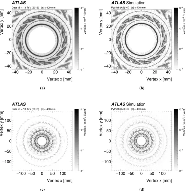
Reconstruction of hadronic interaction vertices enables a detailed visual inspection of the material distribution due to its superb position resolution. Figure 6 shows the distribution of vertices for hadronic interaction candidates in the x-y plane for the data and the Pythia 8MC

simulation for theupdatedsimulation. The qualitative features of the two distributions indicate that

the geometry model description is generally accurate.

6.1 Radial and pseudorapidity regions

For the hadronic interaction and photon conversion analyses, the measurable ID volumes are divided into several groups by radii, which are referred to hereafter asradial regions. Table3lists the radial

regions. The boundaries are chosen to classify distinct barrel layers of the ID. Two regions, referred to as Gap1 (between PIX2 and PIX3) and Gap2 (between PIX3 and PSF), are also introduced as the regions with low purity of hadronic interactions in order to control the background yield of hadronic interaction signals. The gap regions and the other regions overlap so that the number of vertices in the gap regions is increased while also significantly reducing the number of hadronic interactions. For the photon conversion analysis, the regions of IPT, IBL and IST are combined into one region and denoted by “IBL” since the method does not have good enough resolution to differentiate between these components. For the track-extension efficiency study, the η-range is

binned with a bin width of 0.1 for1.5< _|η_| <2.5.

6.2 Radial position offset

In data, the axis of each cylindrical layer of the beam pipe, IBL, pixel barrel layers and other support tubes has an offset perpendicular to thez-axis from the origin of the ATLAS coordinate system due to the placement precision. Figure7ashows the sinusoidal profile of the average radial position of the beam-pipe material as a function ofφ. Similar offsets were observed in a previous

analysis [9,10]. The offset of each layer is estimated by fitting a sinusoidal curve to ther-φprofile.

The obtained size of the oﬀset varies by layers within the range of around0.3mm to1.2mm. The radial distribution of hadronic interaction candidates is compared to the MC simulation in ﬁgure7b

both with and without the application of the radial position corrections.

6.3 Beam pipe

(20)

2017 JINST 12 P12009

(a) (b)

(c) (d)

Figure 6. Distribution of hadronic-interaction vertex candidates in_|η_|<2.4and_|z_|<400 mmfor data and thePythia 8MC simulation with theupdated geometry model. (a),(b)The x-yview zooming-in to the beam pipe, IPT, IBL staves and IST, and(c),(d)of the pixel detector. Some diﬀerences between the data and thePythia 8MC simulation, observed at the position of some of the cooling pipes in the next-to-innermost layer (PIX1), are due to mis-modelling of the coolant ﬂuids, as discussed in ref. [9].

of the geometry model is generally good, but an excess of candidates is observed in data at the centremost part of the beam pipe within_|z_| < 40 mm. The radial distributions of the beam pipe in differentz-ranges are shown in figure9normalised to the rate in the beam pipe at_|z_| > 40 mm. While the radial distribution is well described for_|z| >40 mm, there is a significant excess within

(21)

2017 JINST 12 P12009

Table 3. Deﬁnition of the radial regions used for comparing data to MC simulation. In the case of the

photon conversion analysis, the IPT, IBL and IST regions are always considered together, due to the limited resolution of the approach. The correspondingzregion used for the data to MC simulation comparison is |z_|<400 mmfor all of the radial regions listed.

Radial Region Radial range [mm] Description BP 22.5–26.5 beam pipe

IPT 28.5–30.0 inner positioning tube

IBL 30.0–40.0 IBL staves (for photon conversion: IPT+IBL+IST) IST 41.5–45.0 inner support tube

PIX1 45.0–75.0 ﬁrst pixel barrel layer PIX2 83–110 second pixel barrel layer PIX3 118–145 third pixel barrel layer PSF 180–225 pixel support frame PST 225–240 pixel support tube

SCT-ITE 245–265 SCT inner thermal enclosure SCT1 276–320 ﬁrst SCT barrel layer SCT2 347–390 second SCT barrel layer

Gap1 73–83 material gap between PIX1 and PIX2 Gap2 155–185 material gap between PIX3 and PSF

3

− −2 −1 0 1 2 3

Radial Profile [mm]

23 23.5 24 24.5 25

r = 1.23 mm

δ 1.82 − = 0 φ ) 0 φ − φ r cos( δ + 0

) = r

φ

r(

φ

3

− −2 −1 0 1 2 3

Fit)/Fit − (Data 0.002 − 0 0.002

= 13 TeV s Data

Beam Pipe

ATLAS

(a)

Hadronic Interaction Radius [mm]

20 25 30 35 40 45

Vertices / 0.125 mm

0 10000 20000 30000 40000 50000 60000 BP IPT IBL IST

Data (Corrected) Data (Original)

Had. Int. Fakes

In-flight Decays γ Convs.

ATLAS

= 13 TeV s

|z| < 400 mm

(b)

Figure 7.(a)Ther-φproﬁle of hadronic interaction candidates at the beam pipe, ﬁtted with a sinusoidal curve

to determine the shift of the pipe from the origin of the ATLAS coordinate system in thex-yplane. In the ratio plot in the bottom panel, a small sinusoidal deviation in data from the fit is observed. This may be reflect a slight misalignment of the beam pipe with respect to thez-axis, but this does not affect the result of the analysis. (b)Comparison of the radial distribution of hadronic interaction candidates to theEposupdatedgeometry model before and after the radial offset correction to the data for each barrel layer within20 mm<r <45 mm.

(22)

2017 JINST 12 P12009

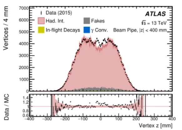
Vertices / 4 mm

0 1000 2000 3000 4000 5000 6000 7000

Vertex z [mm]

400

− −300 −200 −100 0 100 200 300 400 Data / MC 0.6

0.81 1.2 1.4

ATLAS

= 13 TeV s Beam Pipe, |z| < 400 mm Data (2015)

Had. Int. Fakes

In-flight Decays γ Conv.

Figure 8. Comparison of thez-distribution of the rate of hadronic interaction candidates at the beam pipe

in data andEposMC simulation with theupdatedgeometry model. The band shown in the bottom panel indicates statistical uncertainty of the MC simulation.

Vertices / 0.25 mm

0 5000 10000 15000 20000 25000 30000 35000

Vertex Corrected Radius [mm]

22.5 23 23.5 24 24.5 25 25.5 26 26.5

MC) / MC

− (Data 0 2 4 ATLAS 40 mm −

400 mm < z <

−

(Norm. at |z| > 40 mm)

Data (2015) Had. Int. Fakes In-flight Decays Convs. γ

(a)−400 mm<z<−40 mm.

Vertices / 0.25 mm

0 2000 4000 6000 8000 10000 12000 14000 16000

22.5 23 23.5 24 24.5 25 25.5 26 26.5

MC) / MC

− (Data 0 2 4 ATLAS |z| < 40 mm (Norm. at |z| > 40 mm)

(b)|z|<40 mm.

Vertices / 0.25 mm

0 5000 10000 15000 20000 25000

22.5 23 23.5 24 24.5 25 25.5 26 26.5

MC) / MC

− (Data 0 2 4 ATLAS 40 mm < z < 400 mm (Norm. at |z| > 40 mm)

(c)40 mm<z<400 mm.

Figure 9.Comparison between data and simulation of ther-distribution of the hadronic interaction candidates

at the beam pipe (22.5 mm<r<26.5 mm) in diﬀerentzsections. The MC simulation is normalised to the

data using the rate at_|z_|>40 mm. An excess is observed at the outer surface of the beam pipe for_|z_|<40 mm.

6.4 IBL and its support tubes

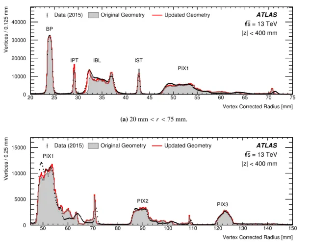
For the IBL staves, the rate of hadronic interactions in the simulation with theoriginalgeometry

model is found to be significantly smaller than in the data aroundr _≃32 mm, as shown in figure10a. A corresponding deficit is observed for photon conversions. Investigations clarified that some surface-mounted components, e.g. capacitors, located on the front-end chips of the IBL modules, are missing in theoriginalgeometry model. As described in section3.3, theupdatedgeometry model

was created to resolve this issue; this gave significantly better agreement with the data. The descrip-tion of the rate as a funcdescrip-tion of radius in31<r <40 mmis not perfect, but this is believed to be due to misalignment of each stave in the data compared to the nominal design. These effects produce a few-hundredµmof smearing, which could explain the difference between the data and the simulation.

The material composition of the IPT and IST is studied with hadronic interaction vertices. The nominal thickness of the IPT is 0.325 mm at _|z| < 311mm. The observed thickness of the tube in terms of the FWHM (full width at half maximum) of the peak (atr = 29mm in ﬁgure 10a),

divided by 2.35, is 0.55 mm for the data, while it is 0.34 mm for the MC simulation, a diﬀerence which is greater than the estimated radial resolution at the IPT radius (0.13 mm). In theupdated

(23)

2017 JINST 12 P12009

updated geometry is improved. For the IST, the rate in data is approximately 16% smaller than

in theoriginalgeometry model, while the thickness in the data and simulation are similar. In the

updatedgeometry model, the density of the IST is also artiﬁcially scaled to give better agreement.

6.5 Outer barrel layers

The pixel barrel layers were refurbished between Run 1 and Run 2, but the material composition is unchanged. The radial distribution of the outer barrel layers is shown in figure10band figure11c. Due to careful investigations of Run 1 data, the distribution is reasonably well described by the MC simulation in all three layers. Nevertheless, some small deficit in the MC simulation observed around r _≃50 mmandr _≃ 86 mmin the hadronic interaction result may indicate that some components are missing from the simulated pixel modules. Furthermore, a discrepancy in the shape of the distribution is apparent in the region of the stave and cabling structures at58 mm<r <72 mmand 96 mm<r <112 mm. An excess in the MC simulation is also observed in the photon conversion measurements in this region (see figure11c). The material composition of the PSF, PST and SCT barrel layers remains unchanged since Run 1. The radial distributions in this range are shown in figures13cand11d, both of which exhibit good agreement. For hadronic interactions, the fraction of background vertices in this outer region is much larger, relative to the inner layers.

6.6 Regions between pixel and SCT detectors

The track-extension eﬃciency_Eext(η), averaged overφ, is shown in ﬁgure12a. The distribution is approximately constant around a value of 95% within_|η_| < 0.5, gradually falling towards a local

minimum of around 83% at _|η_{| ≃} 1.9. The eﬃciency recovers to around 90% at _|η_{| ≃} 2.2, and

then falls again as_|η_|increases further. This structure of_Eext(η)reﬂects the distribution of material as a function of η, as shown in ﬁgure 5. The MC simulation describes the overall structure of

the η dependence, and there is good agreement in the central region of _|η_| < 1. Nevertheless,

discrepancies at the level of a few percent are observed in the forward region. Figure12bshows the average track-extension eﬃciency as a function ofpT, integrated overηandφ. ThepTdependence is also well described by the MC simulation, and the data points are between those of the two MC generators,Pythia8andEpos.

7 Measurement of material in data and MC simulation

An assessment of the accuracy of the geometry model is performed through the comparison of the data and the MC simulation. In this section, the quantitative details of each material measurement are described.

7.1 Hadronic interactions

The ratio of the numbers of hadronic interaction vertices in data andEposMC simulation using

the updated geometry model, referred to as therate ratio, is used as the primary measurement

observable. Two comparisons are presented, the ﬁrst measurement is referred to as theinclusive rate ratio,Rincl_i . It is determined for each radial regionilisted in table3, and deﬁned as:

R_iincl=

ndata_i

(24)

2017 JINST 12 P12009

20 25 30 35 40 45 50 55 60 65 70 75

Vertices / 0.125 mm

0 10000 20000 30000 40000

BP

IPT IBL IST

PIX1

Data (2015) Original Geometry Updated Geometry

= 13 TeV s

|z| < 400 mm ATLAS

(a)20 mm<r<75 mm.

50 60 70 80 90 100 110 120 130 140 150

Vertices / 0.25 mm

0 5000 10000

15000 Data (2015) Original Geometry Updated Geometry

= 13 TeV s

|z| < 400 mm ATLAS

PIX1

PIX2

PIX3

(b)45 mm<r<150 mm.

Figure 10. Comparison of the radial distribution of hadronic interaction candidates between data and

simulation (originalandupdatedsimulations) for(a)20 mm<r <75mm and(b)45 mm<r<150 mm.

wherendata_i represents the number of hadronic interaction candidates in the sample within the radial regioni. The termSBPis the normalisation factor for the MC simulation common to all the radial regions and is derived from the rate observed at the beam pipe. The factorci is the relative track reconstruction efficiency correction to the MC simulation for the radial regioni, which is estimated usingK_S0samples. The numbernMC_i_,_totalis the sum of all hadronic interaction candidates, including true hadronic interactions, combinatorial fakes, in-flight decays and photon conversions. The rate of in-flight decay background vertices is scaled by an appropriate correction factor, following the approach in ref. [9].

The second measurement is thebackground-subtracted rate ratio,R_isubtr:

R_isubtr=

ndata_i ₋SBP·ci·nMC_i_,_BG

SBP·ci·nMC_i_,_had ,

(25)

2017 JINST 12 P12009

Reconstructed Conversion Vertex z [mm]

200

− −150 −100 −50 0 50 100 150 200

Conversion Candidates / 5 mm

0.0 0.5 1.0 1.5 2.0 2.5 3 10 × ATLAS

18 mm < r < 26 mm Beam Pipe Region

= 13 TeV s Data

Pythia8 (A2) Simulation Photon Conversion Background Norm. Uncertainty ⊕ Stat. (a)

Reconstructed Conversion Vertex Radius [mm]

10 15 20 25 30 35 40 45 50

0 10 20 30 40 50 3 10 × ATLAS

|z| < 400 mm

= 13 TeV s Data

Pythia8 (A2) Simulation Photon Conversion Background Norm. Uncertainty ⊕ Stat. BP IBL (b)

Reconstructed Conversion Vertex Radius [mm]

20 40 60 80 100 120 140

0 10 20 30 40 50 3 10 × ATLAS

|z| < 400 mm

= 13 TeV s Data

Pythia8 (A2) Simulation Photon Conversion Background Norm. Uncertainty ⊕ Stat. BP IBL PIX1 PIX2 PIX3 (c)

Reconstructed Conversion Vertex Radius [mm] 160 180 200 220 240 260 280 300 320 340

0.0 0.5 1.0 1.5 2.0 2.5 3 10 × ATLAS

|z| < 400 mm

= 13 TeV s Data

Pythia8 (A2) Simulation Photon Conversion Background Norm. Uncertainty ⊕ Stat. PSF PST SCT-ITE SCT1 (d)

Figure 11. Conversion vertex position distributions for Pythia 8simulation with the updated geometry model compared to data, including(a)the conversion vertexz-position distribution in the beam-pipe radial

region and the conversion vertex radial distributions in(b)the beam-pipe and IBL region,(c)region up to and including the third pixel layer and(d)region between the PSF second SCT layer.

2.5

− −2 −1.5 −1 −0.5 0 0.5 1 1.5 2 2.5

Track-Extension Efficiency 0.75 0.8 0.85 0.9 0.95 1 ATLAS

= 13 TeV s Data 2015 Pythia8 Simulation EPOS Simulation η 2.5

− −2 −1.5 −1 −0.5 0 0.5 1 1.5 2 2.5

MC

−

Data −0.04 0.02

−

0

Data vs Pythia8 Simulation Data vs EPOS Simulation

(a)

0.5 1 1.5 2 2.5 3 3.5 4 4.5 5

Track-Extension Efficiency 0.75 0.8 0.85 0.9 0.95 1 ATLAS

= 13 TeV s Data 2015 Pythia8 Simulation EPOS Simulation [GeV] T p

0.5 1 1.5 2 2.5 3 3.5 4 4.5 5

MC

−

Data −0.02

0

0.02 _{Data vs Pythia8 Simulation} _{Data vs EPOS Simulation}

(b)

Figure 12. Track-extension eﬃciency as a function of (a)η and(b) pT of the tracklets in a comparison

(26)

2017 JINST 12 P12009

is applied to both the signal and the background processes. If the geometry model description is

accurate,Rincl_i andR_isubtrshould be consistent with unity, while any deviation from unity, outside of the measurement uncertainty, may be associated with an inaccuracy in the material description.

Several corrections must be applied to both the data and simulation in order to compare the hadronic interaction rate in data with simulation in a given radial region. In this section, the corresponding systematic uncertainties are discussed. The values of systematic uncertainties are summarised in table6in section8.

7.1.1 Corrections

Radial position of barrel layers. As discussed in section6.2, the barrel layers in data have a ﬁnite

oﬀset perpendicular to thez-axis. In order to compare radial distributions in data and simulation, the positions of secondary vertices in the data are corrected by the oﬀset in the x-y plane. Since

the classiﬁcation of the radial regions is unambiguous after the oﬀset corrections, no systematic uncertainties are assigned to this correction.

Normalisation of rate at the beam pipe. The material in the beam pipe is the part of the

inner detector’s material which is known with the greatest accuracy. Consequently, anin siturate

normalisation using the beam pipe is applied in this study. The geometry model description of the beam pipe at_|z| >40 mm is assumed to be accurate to within 1% precision. The range_|z|< 40 mm

is not used as a part of the reference material due to the observation of a deﬁcit of material in the simulation corresponding to the polyimide tape, as described in section6.3.

Primary interaction reweighting. In order to correct the primary-vertex z-distribution in the

MC simulation, as well as the primary-particle ﬂux, as a function ofη, a reweighting correction is

applied. The track multiplicity density, as a function of the primary-vertexz-position,pTandηof the track, is calculated. The ratio of the spectra in the data and simulation is used as a weight for each secondary vertex. ThepT of the primary particle that created the hadronic interaction vertex cannot be directly determined due to the possible production of undetected neutral particles in hadronic interactions. Instead, the reconstructed vertex’s vectorial sumpTis used to parameterise the correction. The impact of primary-particle reweighting is found to change the data-to-MC simulation rate ratio by less than 1%.

Reconstruction efficiency. The reconstruction eﬃciency is assumed to be qualitatively well

(27)

2017 JINST 12 P12009

Vertices / 50 MeV

1 10 2 10 3 10 4 10 5 10 6 10 7 10

of Tracks [GeV] T

Vectorial Sum p

0 0.5 1 1.5 2 2.5 3 3.5 4 4.5 5

Data / MC 0.6 0.81 1.2 1.4

ATLAS

= 13 TeV s Beam Pipe, |z| < 400 mm

Data (2015)

Had. Int. Fakes In-flight Decays γ Conv.

(a)

Vertices / 50 MeV

1 10 2 10 3 10 4 10 5 10 6 10 7 10

of Tracks [GeV] T

Vectorial Sum p

0 0.5 1 1.5 2 2.5 3 3.5 4 4.5 5

Data / MC 0.6 0.81 1.2 1.4

ATLAS

= 13 TeV s PIX1, |z| < 400 mm

Data (2015)

(b)

150 200 250 300 350 400

Vertices / 0.125 mm

0 200 400 600 800 1000 1200 ATLAS

= 13 TeV s |z| < 400 mm

PSF PST

SCT-ITE SCT1

SCT2

Data (2015) Data (2015)

(c)

Vertices / 0.02

1 10 2 10 3 10 4 10 5 10 6 10 ) op θ cos( 1

− −0.8 −0.6 −0.4 −0.2 0 0.2 0.4 0.6 0.8 1 Data / MC 0.6

0.81 1.2 1.4

ATLAS

= 13 TeV s Gap1, |z| < 400 mm

Data (2015)

(d)

Figure 13. Distribution of the vertex vectorial sum of pT in hadronic interaction candidates(a) at the

beam pipe in 22.5 mm < r < 26.5 mm, and (b) at the innermost pre-existing pixel layer (PIX1) in 45 mm<r <75 mm. (c)Radial distribution of hadronic interaction candidates in150 mm<r <400 mm. Background rates are not weighted for the Epos MC simulation. (d) Distribution of the cosine of the opening angle between two tracks in the laboratory frame cos₍θop)for hadronic interaction candidates within

the material gap at 73 mm < r < 83 mm (Gap1) where fake vertices and in-ﬂight decays are enhanced.

Background rates are not weighted for theEposMC simulation. The band shown in(a),(b)and(d)indicates the statistical uncertainty of the MC simulation.

vertex position due to the lifetime of theK_S0meson. The ratio of the data rate to the MC simulation rate at a given radius after reweighting, 0.97–1.03 depending on radius (see ﬁgure14a), is considered as an estimate of the correction factor to be applied to the vertex reconstruction eﬃciency for the hadronic interaction candidates in the MC simulation.

7.1.2 Description of systematic uncertainty estimation

Physics modelling of hadronic interactions. Modelling of hadronic interactions in theGeant4

simulation is a source of uncertainty in the MC simulation rate, since the acceptance and eﬃciency of the secondary vertex reconstruction depend on the hadronic interaction kinematics. The model used in the simulation,FTFP_BERT, is found to describe the kinematic properties of hadronic interactions

(28)

2017 JINST 12 P12009

Vertex Radius [mm]

20 30 40 50 ₁₀2 ₂_×₁₀2

Efficiency Correction Factor

0.9 0.95 1 1.05 1.1

1.15 ATLAS

= 13 TeV s

| < 2.4 SV η |

Central Value (Data/EPOS)

Total Uncertainty

(a)

Vertices / 0.125 mm

0 5000 10000 15000 20000

30 31 32 33 34 35 36 37 38 39 40

MC / Data 0

0.5 1

Data (2015) Updated Geometry

Updated Geometry (Weighted +10%) Updated Geometry (Weighted -10%)

ATLAS

= 13 TeV s |z| < 400 mm

(b)

Figure 14. (a)The estimated data-to-MC ratio of reconstruction eﬃciency and its uncertainty as a function

of vertex radius. (b)Radial distribution of hadronic interaction candidates at the IBL region (30 mm<r <

40 mm) for the data and thePythia 8MC simulation with theupdatedgeometry model, together with the “IBL+10%” and “IBL−10%” distorted geometry samples listed in table1.

description is not totally accurate, and some diﬀerences are visible in particular at smaller vertex radii. Figures13aand13bshow vectorial sum of pT of the tracks associated with the vertex of hadronic interaction candidates at the beam pipe and at the ﬁrst layer of the pre-existing pixel detector (PIX1) respectively. The description of the distribution of various kinematic variables is found to be generally better at outer radii than at the IBL. The fact that agreement between MC simulation and data for various kinematic distributions is better at outer radii is related to the acceptance of the track reconstruction. At outer radii, the angular phase space is more collimated due to the track reconstruction acceptance, so the kinematic distribution is less dependent on the detailed modelling of the angular distribution of outgoing particles from hadronic interactions.

In order to assess the systematic uncertainty of the hadronic interaction rate associated with the modelling of hadronic interactions forFTFP_BERT, a data-driven approach is taken by varying the

kinematic selection criteria. Four variables (the cosine of the opening angle between two tracks in the laboratory frame cos₍θop), vertex vectorial sum ofpT, leading-trackpT, and sub-leading-track pT) are considered in order to assess the level of agreement between the data and simulation. The degree of agreement is evaluated by comparing the data and simulation rates over the entire spectrum to the integral over the two 50% quantiles of the distribution, where the common quantile threshold for both data and MC simulation is calculated based on the data distribution. The simulation rate is renormalised at the beam-pipe radius (for_|z_| > 40 mm) for each selection. For the beam pipe, the

variation of the data-to-MC simulation rate ratio before renormalisation is taken. The maximum diﬀerence amongst the four kinematic variables is taken as the systematic uncertainty in the physics modelling of the data-to-MC simulation rate ratio in the given radial region. Such a variation is evaluated for the inclusive rate ratio and the background-subtracted rate ratio separately. The estimated uncertainty is 5–18% depending on the radial region.

Background estimation. The purity of hadronic interactions in the sample of hadronic interaction