機械知覚&ロボティクスグループ／中部大学

The Exemplar-SVM (E-SVM) is a learning method based on exemplar that uses only one positive sample and a substantial number of negative samples. In the detection stage, it is possible to detect the location of the target object and estimate the attribute by trans-ferring the attribute of the nearest exemplar. The use of E-SVM classifiers leads to very high computational cost because it is necessary to compute the inner products of weight vectors for multiple classifiers and an input feature vector. For accelerating the com-putation of E-SVM, we propose binary approximation based on matrix decomposition. First, we stack the E-SVM’s weight vectors as a matrix. Then, we decompose the matrix into common binary basis vectors and real-valued coefficient vectors for computing the approximated inner products by logical operation. We also introduce early rejection by cascade structure classifier into the proposed method. The evaluation experiments show that the computation time of the proposed method is lower by a factor of 200 than that of the conventional E-SVM.

1 Introduction

For robust object detection in the various appearances, Exemplar SVM [11] trains classi-fiers such that each instance sample (exemplar) is discriminated from the other samples. The E-SVM classifier has the capability of estimating the attributes of detected objects by transferring the attributes of the nearest exemplar. The E-SVM is also used for 3D object de-tection from point-cloud data in order to estimate 6D object pose [15]. Kobayashi proposed the optimization of the cost parameters for the highly accurate classification of the E-SVM [9]. Also, Modolo proposed an efficient optimization method for calibration by joint calibra-tion [12]. In the training stage of E-SVM, it is necessary to construct classifiers individually

c

(2)

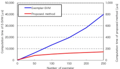
Figure 1: Relationship between the computation time and the number of exemplar.

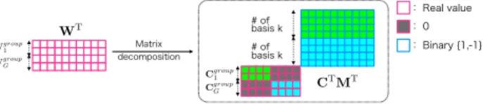
Figure 2: Weight vector decomposition in the E-SVM classifier.

for each positive sample as exemplar. In the detection stage, we apply a raster scanning manner to all trained E-SVM classifiers to compute the classification score. This is why the E-SVM-based object detection needs high computational cost. The computational cost of the E-SVM are increases with increasing number of exemplars as shown in Fig.1.

Our aim with this study is to accelerate the score computation of the E-SVM. Our work was inspired by recent researches on binary approximation such as binary hashing [7][17], binary descriptors [14][10][2] and vector decomposition [8][1][19]. We stack the weight vectors wi (i=1,2, . . . ,E)of each linear SVM to obtain a weight matrix W=

(w1,w2, . . . ,wE)and then decompose the matrix into binary basis vectors that are common

to all exemplars and scaling coefficient vectors, as shown in Fig.2(b). If the feature vector is binary, it can be approximated by calculating of the inner product of the binary basis vectors and the real-valued coefficients. The inner product of the binary feature vector and binary basis vectors is computed by using logic operations and bit counting. This makes it possible to calculate the classification score in a very short time. Also, from the inner product with a coefficients that have a small number of elements, the error relative to the classification score can be reduced while maintaining accuracy. Furthermore, introducing early rejection into the classification process reduces the number of calculations and achieves high-speed E-SVM object detection. Our method can significantly reduce the computation time as shown in Fig.

1. The computation time of the proposed method is independent of the number of exemplars in the case of that exemplars have a high correlation to each weight vectors.

1.1 Related works

(3)

detection with a cascade classifier structure, which was proposed by Viola et al. [16]. The other approach, approximation, includes binary hashing [5] and binary approximation [8][1][3][19]. Dean et al. have proposed a binary hashing-based method that restricts the classifiers to which extracted features are input [5]. Hareet al. proposed binary approxima-tion of classifier calculaapproxima-tions by decomposing the weight vector of the classifier to binary basis vectors and scaling coefficients [8]. This method approximates the inner product cal-culations in the classification process to achieve faster processing. Chenget al. proposed high-speed object detection at 300 fps using binary approximation [3]. Efficient methods of vector decomposition for binary and ternary approximation have been proposed [19][1]. Yamauchiet al. proposed a method of vector decomposition by exhaustive search [19]. This achieves an even lower error in decomposition than that of Hare et al. [8]. Ambai et al. introduced a ternary approximation and data-dependent decomposition [1].

These vector decomposition methods described above are also easily applied to E-SVM as shown in Fig. 2(a). Since the vector decomposition is applied to each exemplar, the number of calculations of the inner product with the feature vector increases in proportion to the number of exemplars. The proposed method called matrix decomposition can reduce the number of calculations by using common binary basis vectors for E-SVM classification as shown in Fig. 2(b). Furthermore, we build cascade structure by successive matrix de-composition and apply early rejection by cascade structure in the raster scan manner at the detection stage.

1.2 Contributions

In this paper, we propose a method for decomposing a matrix for accelerating computation of Exemplar-SVM. The proposed method has three key features as summarized below.

1. Matrix decomposition: The weight matrix Wof E-SVM as shown in Fig.2(b) is decomposed into a coefficient vectors and a binary basis vectors that are common to all exemplars.

2. Grouping of highly correlated weight vectors: Because the binary basis vectors ob-tained by matrix decomposition are common to all of the exemplars, there is little effect for reducing of permissible error when there is no correlation among the exem-plars. Therefore, the highly correlated weight vectors are grouped together to achieve reduction of the permissible error by matrix decomposition. This makes it possible to reduce the number of calculations for the inner product of the binary basis vectors and input feature vector.

3. Early rejection by cascade structure: A classifier cascade is constructed by suc-cessive matrix decomposition. Introducing a rejection decision at each stage in the cascade reduces the computation for the non-target class in the detection processing.

2 Binary approximation based on vector decomposition

The classification score of linear SVM is computed by

(4)

thresholding real valued-HOG features. The papers[1,18] reported that the B-HOG features have almost same classification performance as that of real-valued HOG features. Gener-ally, the linear classifier classifies the detection object classes and the non-detection object classes by thresholding the output of the classification functionF(x). Linear SVM takes a lot of time to classify the classes because it needs to calculate the inner product between the input feature vector and weight vector. For such problems, binary decomposition that decomposes the weight vector into binary basis vectors and coefficient vector to accelerate classification by approximating the inner product has been proposed [8][19][1].

Binary approximation decomposes the weight vectorwof classification functionF(x)(Eq. (1)) into binary basis vectors M= (m1,m2,· · ·,mk)∈ {−1,1}D×k and coefficient vector

c= (c1,c2,· · ·,ck)∈Rk. The classification functionF(x)can be approximated by

F(x) ≈ sign[cTMTx+b] (2)

:= sign

[(

k

∑

i=1

cimTix

)

+b

]

, (3)

wherex is the binary vectorx∈ {−1,1}D_. _k_{is the basis number. Increasing}_k_improves

the approximation of the classification scoreF(x). Because the calculation for the inner product of binary vectors can be replaced by calculation of the Hamming distance, high-speed calculation is possible.

Training for classifiers by Exemplar-SVM builds a weak classifier for the number of exemplarsE. In the detection stage, we compute all scores by inputting the feature vector into each classifier. The exemplar of the classifier that has the highest score is then selected as the final result. If the scores of all of the classifiers are low, the non-target class is output as the final result. When the vector decomposition method is applied to E-SVM classifier, the binary base vectorsMare calculated for each class (Fig.2(a)). Accordingly, the number of times the inner product of feature vectorxandMcis calculated increases by a factor of the number of exemplars inEfor E-SVM classification.

3 Proposed Method

If there is high correlation among the exemplar weight vectorsw, we can consider that the binary basis vectors, M, are also similar. Therefore, we propose a matrix decomposition method in which the weight vectors of all the classes are represented as a single matrix,W, and that matrix is decomposed into a binary basis vectorsMthat are common to all of the exemplars and coefficient vectorsC. By using the common binary basis vectors, it is possible to obtain the inner product of the input feature vectorx andM in a single calculation, so high processing speed can be achieved. A further increase in processing speed is achieved by introducing early rejection based on a cascade E-SVM classifier architecture.

3.1 Matrix decomposition

First, a classifier for each class is trained by SVM to obtain a weight vectorw. Next, the weight vectors for all of the exemplars inE are stacked to construct a weight matrix

W= (w1,w2,· · ·,wE)∈RD×Eas shown in Fig. 2(b). The constructed weight matrixWis

decomposed into binary basis vectorsM= (m1,m2,· · ·,mk)∈ {−1,1}D×k and coefficient

vectorsC= (c1,c2,· · ·,cE)∈Rk×E. We design a cost functionPfor the matrix

(5)

method is explained in detail below.

Matrix decomposition optimizes the binary basis vectorsMand coefficient vectorsCto minimize Eq. (4).

P=||W−MC||2F. (4)

The matrix decomposition algorithm is shown inAlgorithm1which mutually optimizesM

andCto minimize Eq. (4). Cis optimized by applying Eq. (5), which is obtained by the least squares method, fixingM constant.

C= (MTM)−1₍_MT_W_). ₍₅₎

WhenCis fixed, the value ofMis determined to minimizePthat updated by testing binary pattern. Then, the number of combinations required for one iteration isD×2k_because_M

can be optimized at each dimension. This procedure is repeated until there is convergence of the value of the cost functionP. In this optimization,MandCare iterated atLtimes by changing the initial value ofM, in order to avoid the dependency on the initial value of M.

Algorithm 1Matrix decomposition.

functionmatrix_decomposition (W,L,k)

forl=1 toLdo

InitializeMlto a random choice from {-1,1}

InitializeClto a random real number.

repeat

C= (MT_M₎−1₍_MT_W₎

fori=1 toDdo mi= arg min

a∈{−1,1}k

∥wi−aC∥2 F

end for

P=||W−MC||2 F

untilPconverges

end for

From{Ml}and{Cl}, the binary basis matrix and coefficient vectors for which the cost functionPis minimum

are taken as ˆMand ˆC returnMˆ, ˆC

3.2 Grouping of weight vectors in accordance with correlation

The matrix decomposition is most effective for weight vectors that are close to each other because all of the exemplars are represented by single binary basis vectorsM. In practice, the vector distances for the weight matrixWthat is to be decomposed are not necessarily close for all exemplars. Also, the distance of the weight vectorwbefore decomposition may be close to the distance after decomposition. Therefore, the vectors that are to be decom-posed are grouped in accordance with correlation as shown in Fig. 3when decomposition is performed. Here, the proposed method is characterized by two different points between dictionary learning[13]. First in our method, the decomposed matrix M is a binary. Second, in our method, coefficient vectorsCwithin each group are not sparse. The method for con-structing the cascade by grouping and matrix decomposition is described inAlgorithm2, where the number of matrix decompositions equals to the number of basiskare performed for each group. A normalized value for the distance between vectors is used in the grouping. The normalization of the distance between vector wi(i=1,2, . . . ,E) and vector wj(j =

1,2, . . . ,E)is shown in Eq. (6) and Eq. (7).

z = max{||wa||a=i,j}. (6)

d = −

(_||_w

i−wj||

z −1

)

(6)

Figure 3: Matrix decomposition with grouping: Colors indicate grouping of elements in coefficient vectors.

Because the distanced is a real value of −1∼1, the weight vectorswi andwj are the

same whend=1 and have the opposite directions whend=−1. In the grouping process, the threshold valuethcorreandd are used to group the vectors such that vectors for which

|d|>thcorre are placed in the same group. The vectors in the same groupg are stacked as matrixWgroupg . So, weight matrix will beW= (Wgroup1 ,W

group

2 ,· · ·,W

group

G )∈RD×E.

Therefore, all numbers of basisKareG×k.

Algorithm 2Matrix decomposition by grouping weight vectors in accordance with correla-tion.

functionmatrix_decomposition_with_grouping (W,L,k)

Calculate the distances between the weight vectors in the weight matrixWwith Eqs. (6) and (7). Grouping weight vector

{Wgroup₁ ,Wgroup₂ ,· · ·,Wgroup_G } ←W forg=1 toGdo

Optimize ˆMgand ˆCgby calling matrix_decomposition (Wg,L,k)

end for return{_Mˆ_}_,_{_Cˆ_}

3.3 Faster classification by approximated inner product calculation

and early rejection

Our method uses the early rejection approach in the classification process to reduce the num-ber of approximate inner product calculations needed for the non-target class. We therefore describe a method for constructing a cascade of successive matrix decompositions and an early rejection method using a cascade of classifiers in the following sections.

At the detection stage, we calculate the inner product ofxandMCin the detection stage. Here, we must use all basis vectors for approximating the computation of inner product be-causeM andC are optimized by the exhaustive algorithm. Therefor, the approximation calculation cannot be aborted by using each basis vectors. The algorithm is shown in Al-gorithm3., whereM1andC1are calculated by applying the matrix decomposition method

to the weight matrixWin the first stage. In the second and subsequent stages, the matrix decomposition method is applied to the residual matrixR. The residual matrixRcalculate by difference betweenM_n−1Cn−1of the previous stage andW.

(7)

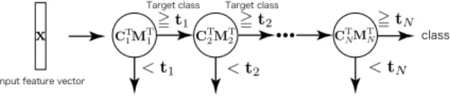
approx-Figure 4: Early rejection in the cascade structure

imate inner product at each stagen. Here, the thresholdt∈RE_{adopts a value that ensures}

the calculated score at theNstage will not be less than -1 because E-SVM is determined to be negative when the score is less than -1.

Algorithm 3 Algorithm for constructing a cascaded classifier by matrix decomposition method.

Require: W,k,N，L

R←W forn=1 toNdo

Optimize ˆMnand ˆCnby calling matrix_decomposition_with_grouping (R,L,k)

R←R−_Mˆ_n_Cˆ_n

end for return{Mˆ},{_Cˆ_}

4 Evaluation experiments

To test the effectiveness of the proposed method, we compared it with the conventional vector decomposition methods [8][19].

4.1 PASCAL VOC 2007 evaluation

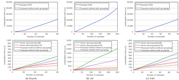
We evaluate computation time and classification accuracy for detection task with dataset in PASCAL VOC 2007[6] in these categories: bicycle, car, and train. For comparing the time required for classification, a personal computer equipped with an Intel Xeon CPU X7542 running at 2.67 GHz. We use the number of basis of the proposed method without grouping that is 11. The basis of the proposed method with grouping is 8.

(8)

Figure 5: Result of number of exemplars vs. computation time: Figure on the top shows a comparison of E-SVM and the proposed method. Figure on the bottom shows a comparison of the conventional vector decomposition method and proposed method

Figure 6: Relationship between classification accuracy and number of basis: True positive rate were plot when the false positive rate = 0.01.

is matrix decomposition with grouping, when category is car. The proposed method is about 200 times faster than E-SVM when the number of exemplars is 250. Fig. 5(c) on the top shows a comparison of E-SVM, and the proposed method, which is matrix decomposition with grouping, when category is train. The proposed method is about 136 times faster than E-SVM when the number of exemplars is 100. Fig.5on bottom shows a comparison of the conventional vector decomposition methods [8][19] and the proposed method. The proposed method is about eight times faster than vector decomposition based on exhaustive algorithm [19]. From Fig. 5, the relationship between computation time and the number of exemplars in E-SVM and the vector decomposition method is linear. Therefore, it takes an immense amount of computation time for classification, when the number of exemplars is large. On the other hand, the processing time of the proposed method is independent of the number of exemplars because the proposed method can save the binary basis vectors. From this, we can say that the proposed method is effective when the number of exemplars is large.

(9)

Figure 7: Data set for toy problem & Comparison of detection accuracy.

4.2 Toy problem evaluation

In this section, we discuss about the following two points: 1. effectiveness of matrix decom-position, and 2. effectiveness of grouping of weight vectors.

We varied the correlation in the matrix that is decomposed and compared the approxima-tion errors of the convenapproxima-tional method and the proposed method (table1). For a matrix of 1,158 dimensions and 27 classes, the correlation between classes was varied from 0.1 to 0.7. The mean square errors when the number of bases was 10 for each stage of the cascade in the

Table 1: Approximation errors.

Method correlation between weight vectors 0.10 0.30 0.34 0.50 0.70 Vector decomposition [8] 7.16 7.10 7.17 7.18 7.92 Vector decomposition [19] 6.02 5.97 5.99 6.00 5.99 Proposed method 11.37 7.89 7.14 4.84 1.97

proposed method, and the number of bases per class was 3 are presented in table1. We can see that a decomposition accuracy that is the same or higher than that for the conventional method is possible for correlation values of 0.34 and above. Because the average correlation of the weight matrixWto be decomposed in the evaluation tests is 0.38, the approximation error is considered to be lower than that for the conventional method.

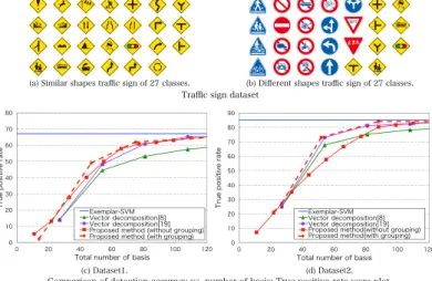
In this experiment, we investigate the effectiveness of grouping of weight vectors with two datasets. Dataset 1 deals with 27 traffic sign images that have similar shapes as shown in Fig.7(a). Dataset 2 deals with 27 traffic sign images that include different shapes as shown in Fig. 7(b). For the positive training samples, we used the traffic sign images modified by changes in geometry and illumination, addition of noise, and compositing. For the samples, we used patch images taken from background images. The training was performed with 500 positive samples and 5,000 negative samples. In evaluating the classification accuracy, 5,000 positive samples and 200,000 negative samples from published data sets were used.

(10)

classification accuracy compared to that of vector decomposition when the number of basis is smaller from Fig. 7(c). In dataset 2, the classification accuracy of matrix decomposition without grouping was degraded compared to vector decomposition when the number of basis is smaller from Fig.7(d). On the other hand, the matrix decomposition with grouping has an improvement in classification accuracy compared to that of vector decomposition and matrix decomposition without grouping, when the number of basis is smaller from Fig.7(d). From this, the matrix decomposition with grouping is effective when the weight vectors are not closed to each other like in dataset 2.

5 Conclusion

(11)

References

[1] Mitsuru Ambai and Ikuro Sato. Spade: Scalar product accelerator by integer decom-position for object detection. InECCV, volume 8693, pages 267–281. Springer, 2014.

[2] Mitsuru Ambai and Yuichi Yoshida. Card: Compact and real-time descriptors. ICCV, pages 97–104, 2011.

[3] Ming-Ming Cheng, Ziming Zhang, Wen-Yan Lin, and Philip Torr. Bing: Binarized normed gradients for objectness estimation at 300fps. InCVPR, 2014.

[4] C. Cortes and V. Vladimir. Support-Vector Networks. InMachine Learning, volume 20, pages 273–297, 1995.

[5] Thomas Dean, Mark A Ruzon, Mark Segal, Jonathon Shlens, Sudheendra Vijaya-narasimhan, and Jay Yagnik. Fast, accurate detection of 100,000 object classes on a single machine.CVPR, pages 1814–1821, 2013.

[6] Mark Everingham, Luc Van Gool, Christopher KI Williams, John Winn, and Andrew Zisserman. The pascal visual object classes (voc) challenge. IJCV, 88(2):303–338, 2010.

[7] Yunchao Gong and Svetlana Lazebnik. Iterative quantization: A procrustean approach to learning binary codes.CVPR, pages 817–824, 2011.

[8] Sam Hare, Amir Saffari, and Philip H.S. Torr. Efficient online structured output learn-ing for keypoint-based object tracklearn-ing.CVPR, pages 1894–1901, 2012.

[9] Takumi Kobayashi. Three viewpoints toward exemplar svm.CVPR, pages 2765–2773, 2015.

[10] Stefan Leutenegger, Margarita Chli, and Roland Yves Siegwart. Brisk: Binary robust invariant scalable keypoints.ICCV, pages 2548–2555, 2011.

[11] Tomasz Malisiewicz, Abhinav Gupta, and A. Alexei Efros. Ensemble of exemplar-svms for object detection and beyond. InICCV, pages 89–96, 2011.

[12] Davide Modolo, Alexander Vezhnevets, Olga Russakovsky, and Vittorio Ferrari. Joint calibration of ensemble of exemplar svms.CVPR, pages 3955–3963, 2015.

[13] Ron Rubinstein, Alfred M Bruckstein, and Michael Elad. Dictionaries for sparse rep-resentation modeling.IEEE, 98(6):1045–1057, 2010.

[14] Ethan Rublee, Vincent Rabaud, Kurt Konolige, and Gary Bradski. Orb: an efficient alternative to sift or surf.ICCV, pages 2564–2571, 2011.

[15] Shuran Song and Jianxiong Xiao. Sliding shapes for 3d object detection in depth im-ages.ECCV, pages 634–651, 2014.

[16] Paul Viola and Michael Jones. Rapid object detection using a boosted cascade of simple features.CVPR, 1:511–518, 2001.

(12)

[18] Y. Yamauchi, C. Matsushima, T. Yamashita, and H. Fujiyoshi. Relational HOG Feature with Wild-Card for Object Detection. InICCV, 2011.