T itle
A S Y MPT OT IC A L L Y UNB IA S E D E S T IMA T ION OF
A UT OC OV A R IA NC E S A ND A UT OC OR R E L A T IONS
W IT H L ONG PA NE L D A T A
A uthor(s )
Okui, R yo
C itation
E conometric T heory (2010), 26(05): 1263-1304
Is s ue D ate
2010-02-17
UR L
http://hdl.handle.net/2433/130692
R ig ht
©
C ambridge University Press 2010; T his is not the published
version. Please cite only the published version. この論文は出
版社版でありません。引用の際には出版社版をご確認ご
利用ください。
T ype
J ournal A rticle
Asymptotically unbiased estimation of autocovariances and
autocorrelations with long panel data
∗
Ryo Okui
†Hong Kong University of Science and Technology
May 27, 2009
∗The author would like to thank two anonymous referees, Guido Kuersteiner, In Choi, Songnian Chen, Masanobu
Taniguchi, Hidehiko Ichimura, Eiji Kurozumi, Peter Phillips, Takashi Yamagata, Katsumi Shimotsu, Stephane Bonhomme, Kohtaro Hitomi, Yoshihiko Nishiyama and seminar participants at Kobe, Hokkaido, Hitotsubashi, Yokohana National, Tokyo and Kyoto Universities, and attendees at the Kansai Econometric Society Meeting held in Yokohama, the Third Symposium on Econometric Theory and Applications held in Hong Kong, the Far Eastern Meeting of the Econometric Society held in Taipei and the 14th Panel Data Conference held in Xiamen. The author also acknowledges financial support from the Hong Kong University of Science and Technology under Project No. DAG05/06.BM16 and from the Research Grants Council under Project No. HKUST643907. The author is solely responsible for all errors.
†Department of Economics, Hong Kong University of Science and Technology, Clear Water Bay, Kowloon, Hong Kong.
Abstract
An important reason for analyzing panel data is to observe the dynamic nature of an economic
variable separately from its time-invariant unobserved heterogeneity. This paper examines how to
estimate the autocovariances of a variable separately from its time-invariant unobserved heterogeneity.
When both cross-sectional and time series sample sizes tend to infinity, we show that the within-group
autocovariances are consistent, although that they are severely biased when the time series length
is short. The biases have the leading term that converges to the long-run variance of the individual
dynamics. This paper develops methods to estimate the long-run variance in panel data settings and
to alleviate the biases of the within-group autocovariances based on the proposed long-run variance
estimators. Monte Carlo simulations reveal that the procedures developed in this paper effectively
reduce the biases of the estimators for small samples.
Proposed running head: Unbiased estimation of autocovariances
Corresponding author: Ryo Okui, Department of Economics, Hong Kong University of Science
1
Introduction
An important reason for analyzing panel data is to observe the dynamic nature of an economic variable
separately from its time-invariant unobserved heterogeneity. In time series analysis, the first step in
investigating the dynamics of a variable may be to examine its correlogram. However, in panel data
analysis, it is difficult to analyze autocovariances and autocorrelations, although some textbooks, such
as Cameron and Trivedi (2005, Chapter 21.3), suggest such an analysis. The difficulty comes from
the fact that sample autocovariances and autocorrelations are contaminated by spurious correlations
caused by unobserved heterogeneity. This paper develops statistical tools to estimate autocovariances and
autocorrelations of economic variables using panel data separately from their time-invariant unobserved
heterogeneity.
When the length of the time series of a panel is short, some restrictions on the autocovariance
struc-ture are necessary, otherwise the autocovariances of the individual dynamics are not identified (see, for
example, Arellano (2003, Chapter 5)) and the conventional autocovariance estimators are even
asymptot-ically biased, as pointed out by Solon (1984). For example, early studies on income dynamics (e.g., Lillard
and Willis (1978), MaCurdy (1982), and Abowd and Card (1989)) model the time-varying components
as ARMA processes. Researchers have developed methods to estimate those models. For
autoregres-sive models, the within-group estimator is severely biased when the length of the time series is short
(Nickell (1981)). Anderson and Hsiao (1981) have proposed instrumental variable estimation of
first-order autoregressive (AR(1)) models. Their methods have been extended by Arellano and Bond (1992)
and Holtz-Eakin, Newey and Rosen (1988) to generalized methods of moments estimation. Baltagi and
Li (1994) consider the estimation of the moving average models. Alternatively, the minimum distance
estimator (see Chamberlain (1984)) may be employed as considered by Abowd and Card (1989).
Recently, panel data with moderately long time lengths have become available, and researchers have
developed mathematical tools to handle asymptotic sequences under which two indexes tend to infinity.
These panels and mathematical tools have motivated researchers to look into the asymptotic properties
of the statistics in the case of long panel data. Alvarez and Arellano (2003) and Hahn and Kuersteiner
(2002) study the asymptotic properties of the within-group estimator for panel AR(1) models when both
the cross-sectional sample size (N) and the length of the time series (T) are large. Kiviet (1995) and Bun and Kiviet (2006) consider more general (but still AR(1)-type) models that include covariates. Hahn
and Kuersteiner (2002) also develop a bias-corrected within-group estimator for panel AR(1) models.
Lee (2008a) and Hansen (2007) consider AR(p) models and develop methods to correct the biases of
the within-group estimators. Lee (2008a) also considers cases in which the lag order is misspecified and
proposes methods to choose the lag order. While AR(p) models can capture many kinds of dynamics,
these methods still suffer from model misspecification. Moreover, the focus of these articles is on the
estimation of the coefficients in autoregressive models, and the results in the existing literature are not
This paper addresses a basic, unanswered question of how to estimate the autocovariance structure
of the individual dynamic component of a variable without imposing a specific structure. The statistical
methods developed in this paper have several potential impacts. They should yield a better understanding
of the dynamic nature of key economic variables. They are also useful for the purpose of finding
appropri-ate models in empirical applications, even if we desire a model-based analysis. Moreover, many important
quantities in dynamic panel data analysis, such as autocorrelations and coefficients in panel VAR models,
are written as a function of autocovariances and understanding how to estimate autocovariances is helpful
in developing methods to estimate those quantities.
We study the asymptotic properties of the within-group autocovariances, using double asymptotics,
under which bothNandT tend to infinity. We show that the within-group autocovariances are consistent for the autocovariances of individual dynamics, but that these estimators are heavily biased when T is only moderately large. The key finding is that the leading terms of the biases of these estimators are
proportional to the long-run variance of the individual dynamics. The presence of long-run variances in
the bias caused by the incidental parameters problem is also observed by Hahn and Kuersteiner (2004)
and Lee (2008a, 2008b).
We consider the estimation of the biases and propose bias-corrected estimators. The key is the
estima-tion of the long-run variance of individual dynamics. There have been numerous procedures proposed for
the estimation of long-run variances in the time series literature. (See, e.g., den Haan and Levin (1997)
for a review, although a large number of articles on this issue has been published since.) We extend the
kernel long-run variance estimators to panel data settings. We then develop methods to alleviate the
biases of the within-group autocovariances using the proposed long-run variance estimator.
We examine the mean squared error (MSE) of the long-run variance estimator and the result reveals
that the bias in the autocovariance estimators also causes bias in the long-run variance estimator. To
address this problem, we consider iterative procedures in which we estimate the long-run variance based
on the bias-corrected estimators of the autocovariances, and we correct the bias using the new
long-run variance estimator. We may repeat this iteration many times. The iteration converges under a
mild condition and the autocovariance estimator obtained as the limit of the iteration has a closed form,
which makes it easy to implement. The theoretical and simulation results show that this iteration reduces
the bias in the long-run estimator and improves the performance of the bias-corrected autocovariance
estimators.
The remainder of the paper is organized as follows. Section 2 introduces the theoretical framework. In
Section 3, we study the asymptotic properties of the within-group autocovariance estimators. Methods to
alleviate the biases of the within-group autocovariance estimators are discussed in Section 4. In Section
2
Setting
Suppose that panel data {yit} for i = 1, . . . , N and t = 1, . . . , T are available. We assume thatyit is generated by the sum of the time-invariant individual effect,ηi, and the time-varying stationary process,
wit:
yit=ηi+wit,
where {{wit}T
t=1}Ni=1 are independently and identically distributed (i.i.d.) across individuals and
sta-tionary over time with mean E(wit) = 0. We do not impose any specific model on the autocovariance structure ofwit.
Let γk denote the k-th order autocovariance of wit (i.e., γk = E(witwit−k)). Our main question is
how to estimateγks when relatively long panel data sets are available.
3
Asymptotic properties of the within-group autocovariances
We examine the asymptotic properties of thek-th within-group autocovariance:
ˆ
γk= 1
N(T−k)
N ∑
i=1
T ∑
t=k+1
(yit−yi¯)(yi,t−k−yi¯),
which may be a natural estimator ofγk, where ¯yi =∑Tt=1yit/T. WhenT is fixed, ˆγk is not consistent for γk (Solon (1984)). The main source of the inconsistency is that we cannot consistently estimate ηi
whenT is fixed. On the other hand, it is shown below that ˆγk is consistent forγk when bothN and T
tend to infinity under the following assumption.
Assumption 1. 1. {{wit}T
t=1}Ni=1 are i.i.d. across individuals.
2. wit is strictly stationary within individuals and ∑∞
j=−∞|γj|<∞.
3. There existsM <∞ such thatE(|witwikwimwil|)< M for anyt,k,mandl.
This set of assumptions is standard. Note that Assumption 1 does not impose any restriction on the
probabilistic nature ofηi, asηi does not appear in ˆγk. The following theorem shows the consistency of ˆ
γk.
Theorem 1. Suppose that Assumption 1 is satisfied. AsN → ∞ and T → ∞, we have γkˆ →p γk for
any k.
However, ˆγk may be severely biased whenT is not very large relative to N. To see this, we observe that ˆγk may be decomposed in the following form (see the proof of Theorem 1):
ˆ
γk = 1
N(T−k)
N ∑
i=1
T ∑
t=k+1
witwi,t−k−
1
N N ∑
i=1
The term ¯wi(= ¯yi−ηi) can be understood as the estimation error for ηi. This estimation error is the main source of the bias, even whenT tends to infinity. Now, we have:
E {
1
N N ∑
i=1
( ¯wi)2
}
=E{( ¯wi)2}= 1
T
γ0+ 2
T−1
∑
j=1
T−j T γj
,
which is of orderO(1/T) when∑∞
j=−∞|γj|<∞. Thus, the estimator ˆγk exhibits bias of orderO(1/T), which may be severe whenT is not very large.
To make the argument more formal, we present the theorem below concerning the asymptotic
distri-bution of ˆγk. We make the following assumption that concerns the cumulants ofwit. Letcum(t1, . . . , tp)
denote thep-th-order cumulant of (wi,t1, . . . , wi,tp).
Assumption 2. ∑∞
j2,...,jp=−∞|cum(0, j2, . . . , jp)|<∞, for p≤8.
We use Theorem 3 of Phillips and Moon (1999) to prove the next theorem. Assumption 2 is used to
guarantee the uniform integrability condition of{∑Tt1=k+1(witwi,t−k−γk)/
√
T}2, which is one of the key
conditions of Theorem 3 of Phillips and Moon (1999). To prove the asymptotic normality, Assumption
2 may be relaxed as long as the uniform integrability condition is met. Assumption 2 is also used
to guarantee the existence of the asymptotic variance of ˆγk and is used later to show the asymptotic properties of the long-run variance estimator.
Theorem 2. Suppose that Assumptions 1 and 2 are satisfied. Then, asN → ∞,T → ∞andN/T3→0,
we have
√
N T (
ˆ
γk−γk+ 1
TVT )
→dN
0,
∞
∑
j=−∞
{ γ2
j +γk+jγk−j+cum(0,−k, j, j−k)}
,
where
VT ≡γ0+ 2
T−1
∑
j=1
T−j T γj.
Remark 1. LetV ≡∑∞
j=−∞γj denote the long-run variance ofwit. We haveVT →V asT → ∞. The leading term of the bias of ˆγk converges to the long-run variance ofwit. The next section examines the possibility of correcting the bias by estimating the long-run variance. This observation also implies that
the bias is large ifwitis highly persistent. Note thatVT >0, which implies that the bias is downward and ˆ
γk is, on average, smaller thanγk. It is also notable that the leading term of the bias does not depend on the order of the autocovariance,k.
Remark 2. The condition N/T3→0 is required to ignore the bias term of order 1/T2. This condition
can be relaxed if the bias term of order 1/T2is taken into account. However, it makes the expression of
the asymptotic bias complicated and we shall keep the conditionN/T3→0.
Remark 3. Although this paper is about the bias correction, the efficiency issue might deserve some
to p-th-order are efficient when the process follows a Gaussian AR(p) model (see, e.g., Porat (1987), Kakizawa and Taniguchi (1994) and Kakizawa (1999)). Since ˆγk is the sample average of individual autocovariances and we assume that we have an i.i.d. sample, we may expect that the variance of ˆγk
is the smallest possible when wit follows a Gaussian AR(p) model and k ≤p. This may be proved by following the steps used for the efficiency result in Hahn and Kuersteiner (2002). However, this is beyond
the scope of this paper.
Remark 4. Theorem 2 presents the asymptotic distribution of ˆγk for eachk. It is easy to find the joint asymptotic distribution of ˆγk and ˆγj fork̸=j, because ˆγk has an asymptotic linear form:
√
N T (
ˆ
γk−γk+ 1
TVT )
= √1
N T N ∑
i=1
T ∑
t=k+1
(witwi,t−k−γk) +op(1).
Note that the asymptotic covariance between ˆγk and ˆγj is: ∞
∑
t=−∞
{γtγt−k+j+γt+jγt−k+cum(0,−k, t, t−j)}.
4
Bias correction
In this section, we consider ways to alleviate the bias of γk. We propose to use an estimate of VT to mitigate the bias ofγk. Before discussing how to estimate VT, we show that this idea of bias correction works at least theoretically. Let ˆVT denote an estimator of VT. The bias-corrected estimator of γk, denoted as ˜γk, is obtained by adding ˆVT/T to ˆγk:
˜
γk = ˆγk+ 1
TVTˆ .
LetrN,T be the inverse of the rate of convergence of ˆVT such that ˆVT−VT =Op(rN,T). The next theorem shows that the asymptotic distribution of ˜γk is centered around zero.
Theorem 3. Suppose that Assumptions 1 and 2 are satisfied. Suppose also that N/T3 → 0 and
rN,T√
N/T→0. Then, asN → ∞andT → ∞,
√
N T(˜γk−γk)→dN
0,
∞
∑
j=−∞
{
γj2+γk+jγk−j+cum(0,−k, j, j−k)}
.
The proof is omitted as it is trivial. This theorem implies that we may obtain estimates of the
autocovariances whose biases are small if we get some estimates ofVT. Thus, the main question of this section is how to construct a good estimator of the long-run variance of wit and discover the rate of convergence of the long-run variance estimator.
4.1
Estimating the long-run variance
autocovariances does not yield a consistent estimator. We must weight the effect of the higher-order
autocovariances downward in order to obtain a consistent estimator for the long-run variance. Following
Parzen (1957) and Andrews (1991), we consider the kernel estimators:
˜
VT =
T−1
∑
j=−T+1
k (j
S )T
− |j|
T γjˆ = T−1
∑
j=−T+1
k (j
S )
ˆ
γj+,
where
ˆ
γj+= 1
N T N ∑
i=1
T ∑
t=|j|+1
(yit−yi¯)(yi,t−|j|−yi¯) =
T− |j|
T γjˆ
is the within-group autocovariance usingT in the denominator instead ofT− |j|,k(·) is a kernel function and the scalar,S, is the bandwidth chosen by the researcher. We assume that the kernel function belongs to the classK1:
K1 =
{
k(·) :R→[−1,1]|k(0) = 1, k(x) =k(−x)∀x∈R, ∫ ∞
−∞
k2(x)dx <∞, k(·) is continuous almost everywhere and at 0}.
An example of a kernel that belongs toK1 is the quadratic spectrum (QS) kernel:
k(x) = 3 (6πx/5)2
{
sin(6πx/5)
6πx/5 −cos(6πx/5)
} .
Andrews (1991) demonstrates several attractive properties of the QS kernel function. Note that ˜VT is always nonnegative with the QS kernel, which also means that ˜γ0 is nonnegative with the QS kernel.
Later, we also consider the truncated kernel:
k(x) =
1 if|x| ≤1,
0 otherwise.
We also assume that the kernel function satisfies∫
k(x)dx <∞and∫
|x|k(x)dx <∞.
The following theorem shows the consistency of ˆVT and gives the rate of convergence of ˆVT. The MSE formula given in the theorem also serves as the device used to choose the bandwidth parameter.
Theorem 4. Suppose that Assumptions 1 and 2 are satisfied. Assume that k(·) ∈ K1,
∫
k(x)dx <∞
and∫
|x|k(x)dx <∞. IfS→ ∞ andS/T →0, then,
˜
VT −VT →p0.
Let kq ≡ limx→0{1 −k(x)}/|x|q and V(q) = ∑∞j=−∞|j|qγj. Suppose also that Nq+1/Tq → 0 and
S2q+1/(N T)→τ, where0< τ <∞, for some0< q <∞, for which kq and|V(q)| are finite. Then,
lim
N,T→∞
N T
S M SE( ˜VT) =k
2
q (
V(q))2τ−1+ 2V2 ∫
On the other hand, suppose thatNq+1/Tq→ ∞andSq+1/T →τ, where0< τ <∞, for some0< q <∞,
for whichkq and|V(q)|are finite. Then,
lim
N,T→∞
T2
S2M SE( ˜VT) =
{
−kqV(q)τ−1−V
∫
k(x)dx }2
.
The value ofqin the theorem represents the smoothness of the kernel function at the origin. A large value ofqfor whichkq is finite indicates that the kernel function is smooth at zero. For example, the QS kernel hasq= 2.
Remark 5. There are two bias terms that are relevant to this result. The first bias term that is
proportional to kqV(q) comes from the fact that we use a kernel function. The other bias term that is
proportional to V∫
k(x)dx stems from the result that each ˆγk is biased. When T is sufficiently large relative to N (i.e., Nq+1/Tq →0), the MSE has a similar form to that presented by Andrews (1991). WhenT is not very large compared withN (i.e.,Nq+1/Tq → ∞), the second term of the bias becomes
more important than the variance term. Note that the estimator, ˆVT, is the sample average of the long-run variance estimators across individuals and thatN affects the variance, but not the bias, of ˆVT. Therefore, whenN is large, the variance becomes small relative to the biases and the leading term in the MSE is the square of the leading terms of the biases. This phenomenon happens whenN is proportional toT and is relevant in practice.
Remark 6. The theorem gives the rate of convergence of ˆVT, which is useful in examining the conditions on the relationship betweenNandTfor asymptotically unbiased estimation of autocovariances. Theorem 3 assumes two conditions, N/T3 →0 and rN,T√
N/T →0. Theorem 4 gives rN,T = (N T)−q/(2q+1) if
Nq+1/Tq→0, andrN,T =T−q/(q+1)ifNq+1/Tq → ∞. WhenNq+1/Tq→0, the conditionN/T3→0 is
automatically satisfied andrN,T√
N/T = (N/T4q+1)1/(4q+2), which is alsoo(1) underNq+1/Tq→0. On
the other hand,N/T3→0 is stronger thanNq+1/Tq → ∞and the conditionrN,T√
N/T →0 becomes (Nq+1/T3q+1)1/(2q+2)→0, which is stronger thanN/T3 →0. Therefore, we need Nq+1/T3q+1→0 for
asymptotically unbiased estimation of autocovariances if we correct the bias by using ˜VT.
4.2
Choosing the bandwidth parameter
We choose the bandwidth parameter by minimizing the MSE of ˜VT. Letξ=V(q)/V. Then, the value of
the bandwidth parameter that minimizes the MSE is:
S∗=
[
{qk2
q/ ∫
k2(x)dx}ξ2T N]1/(2q+1)
, whenNq+1/Tq →0,
[
{qkq/∫
k(x)dx}ξT]1/(q+1)
, whenNq+1/Tq → ∞andV(q)≥0,
[
{kq/∫
k(x)dx}|ξ|T]1/(q+1)
, whenNq+1/Tq → ∞andV(q)<0.
We need to obtain an estimate of ξ. We follow the strategy proposed by Andrews (1991): we estimate
process with coefficientδ, then the parameterξ can be written as:
ξ= 2δ (1−δ)2.
There are many ways to estimate the parameter δ. Here, we consider the estimator in Hahn and Kuer-steiner (2002):
ˆ
δ= T
T−1
∑N i=1
∑T
t=2(yi,t−1−yi¯−)(yi,t−1−yi¯+)
∑N i=1
∑T
t=2(yi,t−1−yi¯−)2
+ 1
T−1,
where ¯yi− =∑Tt=1−1yit/(T−1) and ¯yi+ =∑Tt=2yit/(T−1). Then, we estimateξ by ˆξ= 2ˆδ/{(1−δˆ)2}.
We use the following estimated bandwidth:
ˆ
S∗=
min
{[
{qk2
q/ ∫
k2(x)dx}ξˆ2T N]1/(2q+1),[{qkq/∫
k(x)dx}ξTˆ ]
1/(q+1)}
, if ˆξ≥0,
min
{[
{qk2
q/ ∫
k2(x)dx}ξˆ2T N]1/(2q+1),[{kq/∫
k(x)dx}|ξˆ|T]1/(q+1) }
, if ˆξ <0.
Note that ˆδ converges to the first-order autocorrelation of wit and is bounded in probability. Thus, the estimation of ˆδ (and ˆξ) does not affect the rate of the bandwidth asymptotically. We see that
C1(T N)1/(2q+1)< C2(T)1/(q+1)forT andN sufficiently large for any constantsC1andC2ifNq+1/Tq→
0 and the opposite result holds ifNq+1/Tq → ∞. These observations imply that
Pr
{
ˆ
S∗=
[{ qkq2/
∫
k2(x)dx }
ˆ
ξ2T N
]1/(2q+1)}
→1 if Nq+1/Tq →0,
Pr
{
ˆ
S∗=
[{ qkq2/
∫
k2(x)dx }
ˆ
ξ2T N
]1/(2q+1)}
→0 if Nq+1/Tq → ∞.
Thus, the bandwidth has an appropriate rate in large samples.
In the simulations, we use the QS kernel function, for which we haveq= 2,kq ≈1.4212,∫
k(x)dx≈
1.2930 and∫
k2(x)dx= 1. The bandwidth is:
ˆ
S∗=
min{1.3221( ˆξ2T N)1/5,1.3002( ˆξT)1/3}, if ˆξ≥0,
min{1.3221( ˆξ2T N)1/5,1.0320(|ξˆ|T)1/3}, if ˆξ <0.
(1)
Remark 7. One may alternatively consider choosing the bandwidth parameter by minimizing the MSE of
˜
γk. In general, the bandwidth parameter that minimizes the MSE of ˜γk is different from that minimizing the MSE of ˜VT. However, the benefit of using this alternative criterion is limited. To see this, consider the MSE of ˜γk:
E{(˜γk−γk)2}=E
{ (
ˆ
γk−γk+ 1
TVT )2}
+ 21
TE {(
ˆ
γk−γk+ 1
TVT )
( ˜VT −VT)
}
+ 1
T2E{( ˜VT −VT) 2}.
While the cross term,E{(ˆγk−γk+VT/T) ( ˜VT−VT)}/T, depends on the bandwidth, its leading term does not. The cross term is approximately equal to∑Tj=−−1T+1k(j/S)cov(ˆγk,ˆγj)/T. SinceN T∑Tj=−−1T+1cov(ˆγk,γjˆ ) converges, we have
1
TE {(
ˆ
γk−γk+ 1
TVT )
( ˜VT −VT)
}
=O (
1
N T2
which implies that the bandwidth does not affect the order of the cross term. Moreover, when N is relatively large, the cross term is small compared with the MSE of ˜VT. For example, whenN3/T4→ ∞,
the order of the term E{( ˜VT −VT)2}/T2 with the QS kernel is T−2−4/3 = T−10/3 and is of an order
larger thanO(1/(N T2)).
4.3
Iterative procedures
Theorem 4 demonstrates that the bias in each ˆγk is relevant even in the estimation of the long-run variance. To address this problem, we use an iterative procedure. We update the estimate of VT using the bias-corrected estimators for γk fork= 0, . . . , T−1. Then, we reestimate γk based on the updated estimate ofVT. This iteration may be repeated many times. As ˜γks are bias-corrected, we expect that the long-run variance estimator based on ˜γk is also bias-corrected. The iteration is expressed in the following way. Let
˜
VT(m+ 1) =
T−1
∑
j=−T+1
k (
j Sm
) T− |j|
T ˜γj(m),
and
˜
γk(m) = ˆγk+ 1
TVT˜ (m), k= 0, . . . , T−1,
where m denotes the number of iterations, Sm is the bandwidth parameter for the m-th iteration and ˜
γk(0) = ˆγk fork= 0, . . . , T−1.
Let ˜γ(m) = (˜γ0(m), . . . ,˜γT−1(m))′, ˆγ= (ˆγ0, . . . ,ˆγT−1)′, IT be theT ×T identity matrix and ιT be
theT×1 vector of ones. We consider using the same bandwidth throughout the iterations. LetSdenote the bandwidth parameter. Let
KT =
(
k(0),2T −1
T k (
1
S )
,2T −2
T k (
2
S )
, . . . ,21
Tk (
T−1
S ))′
.
We can write the iteration formula in the following way:
˜
γ(m+ 1) = ˆγ+ 1
TιTK
′
Tγ˜(m).
Ifι′TKT < T, this iteration converges and the limit, ˜γ(∞), can be written as
˜
γ(∞) =
(
IT + 1
T−ι′
TKT ιTKT′
)
ˆ
γ=
(
IT−T1ιTKT′ )−1
ˆ
γ.
Note that ι′
TKT < T is satisfied when k(x) < 1 for x ̸= 0. Most commonly used kernel functions,
including the QS kernel, satisfy this condition. The long-run variance estimator obtained as the limit of
the iteration is
˜
VT(∞) =K′
Tγ˜(∞) =KT′ (
IT + 1
T−ι′
TKT ιTK′
T )
ˆ
γ=
(
1 + ι ′
TKT T−ι′
TKT )
˜
The following theorem presents the MSE of ˜VT(∞). Since ˜VT(∞) is based on the bias-corrected autocovariance estimators, the second term in the bias becomes small, and we have the usual bias–
variance trade-off. Note that the iterations do not alter the asymptotic distribution of ˜γs, while the rate conditions forN andT would be affected.
Theorem 5. Suppose that Assumptions 1 and 2 are satisfied. Assume that k(·) ∈ K1, ∫ k(x)dx <∞
and ∫
|x|k(x)dx < ∞. Suppose also that S → ∞ andS/T → 0. Then, VT˜ (∞)−VT →p 0. Let q be a
number that satisfies0< q <∞, for whichkq and|V(q)| are finite. Then, asN → ∞ andT → ∞with
Nq+2/T3q→0 andS2q+1/(N T)→τ, we have:
lim
N,T→∞
N T
S M SE{VT˜ (∞)}=k
2
q (
V(q))2τ−1+ 2V2 ∫
k2(x)dx.
Remark 8. One of the conditions for ˜γk to be asymptotically unbiased is rN,T√N/T = o(1), which is automatically satisfied since rN,T = (N T)−q/(2q+1) and Nq+1/T3q → 0 under the conditions of the
theorem. On the other hand, Nq+2/T3q →0 is typically stronger than N/T3 → 0 because commonly
used kernel functions have q = 1 or q= 2. For example, the QS kernel has q = 2 and asymptotically unbiased estimation of autocovariances is possible under N2/T3 →0 when the bias correction is done
using ˜VT(∞) with the QS kernel.
Remark 9. The estimator ˜γ(∞) may be motivated as a continuously updated estimator ofγ= (γ0, . . . , γT−1)′.
We note thatE(ˆγ)≈γ−ιTVT/T. By replacingVTwithK′
Tγ, we getE(ˆγ)≈γ−ιTKT′γ/T. The estimator
˜
γ(∞) can be obtained by solving the following equation: ˆγ= ˜γ(∞)−ιTK′
T˜γ(∞)/T.
As before, we use the MSE formula as the device to choose the bandwidth parameter. The bandwidth
parameter that minimizes the MSE formula is
S∗=
[{ qk2q/
∫
k2(x)dx }
ξ2T N
]1/(2q+1) .
For the QS kernel function, the bandwidth parameter may be chosen to be:
ˆ
S∗= 1.3221( ˆξ2T N)1/5. (2)
4.4
The truncated kernel
In this subsection, we discuss the bandwidth choice rule for the truncated kernel. Let ˇVT and ˇVT(∞), respectively, be the long-run variance estimator and its infinitely iterated version based on the truncated
kernel such that:
ˇ
VT =
S ∑
j=−S T− |j|
T ˆγj = S ∑
j=−S
ˆ
γj+,
ˇ
VT(∞) =
(
1 + ι ′
TKT∗ T−ι′
TKT∗ )
ˇ
whereK∗
T = (1,2(T−1)/T, . . . ,2(T−S)/T,0, . . . ,0). The truncated kernel has not been commonly used
in long-run variance estimation. The main reason is that the truncated kernel does not guarantee the
positive definiteness of the estimator. However, as pointed out by Hahn and Kuersteiner (2007), ensuring
the positive definiteness may not be important if the purpose of estimating the long-run variance is the
bias correction. Given that the truncated kernel provides a good estimate whenwit is an M-dependent process, it is worthwhile to consider the truncated kernel in our context.
The bandwidth choice rules in the previous subsections are not useful for the truncated kernel. We
note thatkq = 0 for any finiteqfor the truncated kernel since it is flat around the origin. Therefore, the bias term of orderS−q disappears from the MSE formula and the bandwidth choice rule presented above
recommends that the bandwidth be as small as possible, which obviously does not work in practice.
This observation implies that we need alternative MSE formulas. The following theorem presents the
leading terms of the MSEs of ˜VT and ˜VT(∞). The proof is in the Appendix.
Theorem 6. Suppose that Assumptions 1 and 2 are satisfied. Suppose also thatS → ∞ andS/T →0. Then, VTˇ −VT →p0 and
M SE( ˇVT) =
−2
∞
∑
j=S+1
γj−2V S T
2
+ 4V2 S N T +o
∞
∑
j=S+1
γj
2
+S
2
T2 +
S N T
.
We also haveVTˇ (∞)−VT →p0 and
M SE{VTˇ (∞)}= 4
∞
∑
j=S+1
γj
2
+ 4V2 S N T +o
∞
∑
j=S+1
γj
2
+ S
N T
+O
( S4
T4
) .
The theorem does not explicitly give the rate of convergence of the estimators because it is difficult
to evaluate the order of the term∑∞ j=S+1γj.
We choose the bandwidth using the MSE formulas. As before, we estimate the approximate MSEs
based on the formula that is valid whenwitfollows the panel AR(1) process. Letδbe the AR(1) coefficient and ˆδ be Hahn and Kuersteiner’s (2002) estimator. In the AR(1) model, we have V = (1 +δ)/(1−δ) and∑∞
j=S+1γj=δS/(1−δ). Thus, the bandwidth choice rule for ˇVT is
ˆ
S∗= arg min
S∈{1,...,T−1}
(
−2 ˆδ
S
1−δˆ−2
1 + ˆδ
1−δˆ S T
)2
+ 4
(
1 + ˆδ
1−ˆδ )2
S
N T, (3)
and that for ˇVT(∞) is
ˆ
S∗= arg min
S∈{1,...,T−1}4
(
ˆ
δS
1−ˆδ )2
+ 4
(
1 + ˆδ
1−ˆδ )2
S
N T. (4)
These bandwidth choice rules are similar to that considered by Hahn and Kuersteiner (2007). In
partic-ular,∑∞
j=S+1γj is difficult to estimate in panel data settings and the idea of using an AR(1) model to
5
Monte Carlo simulations
This section reports the results of Monte Carlo simulations. The simulations are conducted on Ox 5.10
(Doornik (2007)).
5.1
Design
The data-generating process used in the experiments is the following:
yit=wit+ηi,
whereηi∼i.i.d.N(0, σ2
η), andwit follows an AR(1) process:
wit=αwi,t−1+ϵit,
andϵit∼i.i.d.N(0, σ2). The initial observations are generated from the stationary distribution.
Specifi-cally, we generate (wi0, ϵi0) from:
wi0
ϵi0
∼N
0,
σ2 1
1−α2 σ 2
σ2 σ2
.
We set the value of σ2 such that γ
0 = 1 (i.e., σ2 = 1−α2) and fix the value of ση2 at ση2 = 1. Note
that σ2
η does not affect the results as ηi is eliminated in the estimation of autocovariances. The value
of σ2 only affects the scale of the estimator and does not have any essential effect on the Monte Carlo
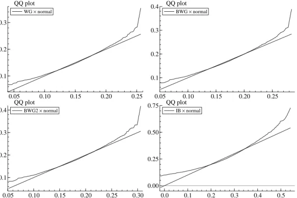
results. Each experiment is characterized by the vector of (N, T, α). We set N = 20; T = 5,10,25,50; andα= 0,0.5,0.9. We consider several different procedures. The first procedure considered is the within-group autocovariances (i.e., ˆγk; we call these “WG”). The other procedures are bias–corrected estimators. The QS kernel and the truncated kernel are used in the bias correction. For each kernel, we consider three
different procedures: the one-time bias-corrected autocovariance (i.e., ˜γk(1); we call these “BWG”); the two-time bias-corrected autocovariance (i.e., ˜γk(2); we call these “BWG2”); the autocovariance estimators obtained after infinite iterations (i.e., ˜γk(∞); we call these “IB”). The bandwidth parameters for the QS kernel are chosen using formula (1) for “BWG” and formula (2) for “IB”. For “BWG2”, the first iteration
uses formula (1) and the second iteration uses formula (2). Similarly, the bandwidth parameters for
the truncated kernel are chosen using formula (3) for “BWG” and formula (4) for “IB”. Formula (3) is
used for the first iteration of “BWG2” and formula (4) is used for the second iteration. The number of
replications is 5000.
We have also tried other specifications whose results are not reported here. Those results are obtained
from the author upon request and are briefly summarized here. We have tried cases where (wi0, ϵi0) = 0
for allithroughout the simulations. However, the specification of the initial observation does not appear to affect the simulation results. We have considered other cross-sectional sample sizes. The results
cross-sectional sample size affects the standard deviations of the estimators. We have also considered
cases in whichwitfollows an ARMA model. The results from the ARMA model are similar to the results we present here.
5.2
Results
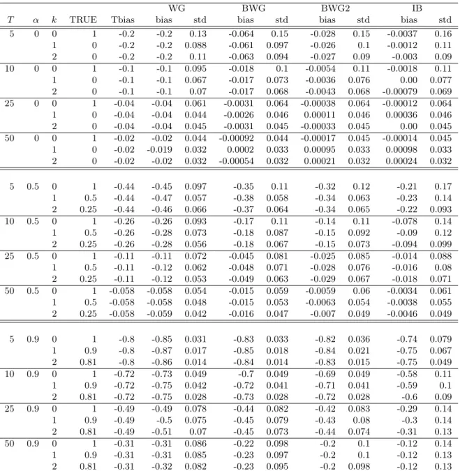
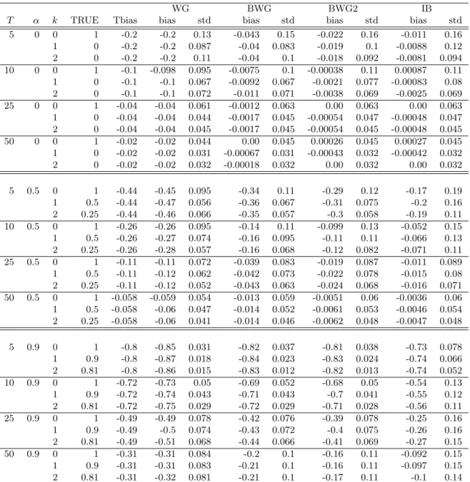
Tables 1 and 2 summarize the results of the experiments. Table 1 presents the results for the QS kernel
and Table 2 presents the results for the truncated kernel. For each procedure, we report the biases and
standard deviations (std) of the estimates of the zeroth-, first- and second-order autocovariances. We
also report the theoretical approximation of the bias of ˆγk (i.e.,VT/T) in the column entitled “Tbias”.
[Tables 1-2 about here]
We first examine the results for “WG”. The biases of “WG” are large when the length of the time
series is short and when the degree of persistence is large (α= 0.9). These findings are consistent with our theoretical results. Moreover, “Tbias” and the biases of “WG” are reasonably similar.
Next, we investigate the performance of the procedures developed in this paper that have bias-reducing
properties. While the “BWG” procedure alleviates the bias, the “BWG2” procedure mitigates the bias
more effectively than does “BWG”. The gain from iterating the bias correction is substantial, particularly
whenT is small (T = 5 and 10). The “IB” procedure eliminates the bias even more effectively than does “BWG2”, although “IB” exhibits somewhat larger standard deviations when T = 5 or α = 0.9. The effectiveness of our bias correction crucially depends on T and α. (In the current setting, αmeasures the persistence of individual dynamics.) When there is no persistence in individual dynamics (α= 0), our bias correction works very well and can completely eliminate the bias even ifT is small. Moreover, whenα= 0, the bias correction does not inflate the standard deviation by much. However, when there is strong persistence (α= 0.9), a long time series is required to obtain estimates that are mostly unbiased and the standard deviations of the bias-corrected estimators are somewhat large compared with “WG”.
Nevertheless, our procedures (in particular, “IB”) are able to improve the within-group autocorrelation
estimators substantially. Compared with the QS kernel, the truncated kernel typically yields a better
bias correction. On the other hand, the choice of the kernel function does not have a large impact on the
standard deviations.
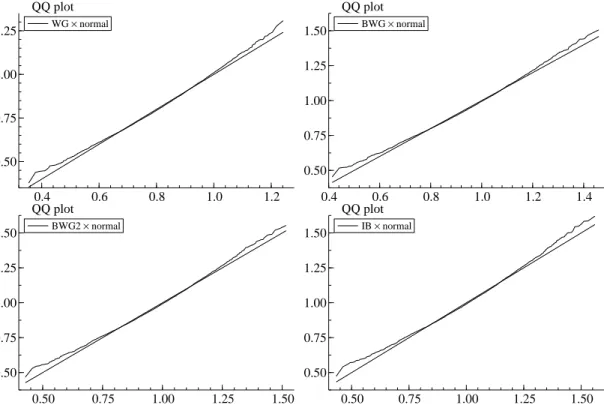
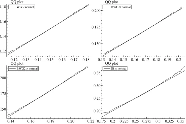
[Figures 1-3 about here]
Lastly, we evaluate the quality of the normal approximation. We compare the distribution of each
estimator with the QS kernel for γ0 with the normal distribution with same mean and variance using
normal distribution considerably. Nonetheless, in Figure 3, we see that the normal approximation works
(although the distributions are not centered around the true value due to the bias) when the sample size
is reasonably large even if the degree of persistence is high.
To sum up, we observe that the procedures developed in this paper effectively reduce the biases. They
provide reliable estimates of the autocovariances, particularly when the time dimension is moderately
large or when the persistence is not very large. On the other hand, when the length of the time series
is short and the persistence is large, our procedures may not be able to eliminate the biases completely,
although they perform remarkably better than does the conventional procedure. We also see that the
asymptotic normal approximation is accurate in sample sizes that we often encounter. Given the results
of the experiments, we believe that applied researchers could benefit by using the procedures developed
in this analysis. In particular, the “IB” procedure with the truncated kernel works remarkably well.
6
Extensions
In this section, we consider several extensions of the methods developed in this paper.
6.1
Other related quantities
We consider the estimation of other related quantities and see how the estimators developed in the
previous sections are useful for this purpose.
Let ρk be the k-th-order autocorrelation ofwit (i.e.,ρk =γk/γ0). We consider estimating ρk based
on estimates ofγk andγ0. Let ˜ρk be the estimator forρk based on bias-corrected estimators:
˜
ρk =γk˜ ˜
γ0.
It is easy to see that ˜ρk is consistent by the continuous mapping theorem. It is also easy to see that, by the Delta method, ˜ρk is asymptotically normal with zero mean.
Partial autocorrelation is another popular measure of dependence over time. Let αk signify thekth partial autocorrelation. Note thatαkis the population value of the coefficient onwi,t−k in the regression
ofwitonwi,t−1, . . . wi,t−k (this does not mean thatwit follows an AR(k) model). We recommend using
bias-corrected estimators of γs to estimate αk. The estimator, ˜αk, is obtained by solving the following equation:
∗ ∗
. . .
˜
αk
=
˜
γ0 γ˜1 . . . γk˜ −1
˜
γ1 γ˜0 . . . γk˜ −2
. . . .
˜
γk−1 γk˜ −2 . . . γ˜0
−1
˜
γ1
˜
γ2
. . .
˜
γk
,
Remark 10. The results in Lee (2008a) can be used to find the probability limit and the asymptotic
distribution of a partial autocorrelation coefficient estimator based on ˆγs (not ˜γ). However, we cannot use the bias correction method by Lee (2008a) for the estimation of the partial autocorrelations. The
strategy that Lee (2008a) adopts is to select the correct order of the autoregression and then mitigate
the bias of the estimates of the coefficients in correctly specified AR (p) models.
Lastly, we consider the variance of individual effects. Letσ2
ηbe the variance ofηi. A natural estimator
ofσ2
η may be the between-group variance:
ˆ
σ2η=
1
N−1
N ∑
i=1
(¯yi−y¯)2,
where ¯y =∑Ni=1∑Tt=1yit/(N T). As for ˆγk, we show below that ˆσ2
η exhibits bias whose leading term
converges to the long-run variance of wit. However, it turns out that the direction of the bias of ˆσ2
η is
upward. A bias-corrected estimator ofσ2
η may be given as
˜
σ2η= ˆση2−
1
TVTˆ .
We need assumptions on the distribution of ηi in addition to the assumptions on wit to study the asymptotic properties of the ˆσ2
η and ˜ση2.
Assumption 3. 1. {ηi}N
i=1 are i.i.d. across individuals.
2. E(η4
i)<∞.
3. wit andηi are independent for anyt.
Theorem 7. 1. Suppose that Assumptions 1 and 3 are satisfied. Then, as N → ∞ andT → ∞, it follows that ˆσ2
η →p ση2.
Suppose that Assumptions 1, 2 and 3 are satisfied. Then, as N→ ∞,T → ∞,
√
N (
ˆ
σ2
η−ση2−
1
TVT )
→dN(0,[E{(ηi−µ)4} −σ4η ])
.
2. Suppose that Assumptions 1, 2 and 3 are satisfied. Suppose also thatrN,TT−1√N →0. Then, as
N → ∞,T → ∞,
√
N(
˜
σ2η−σ2η )
→dN(0,[E{(ηi−µ)4} −ση4 ])
.
Remark 11. WhileT → ∞is required for the consistency of ˆση2, the rate of convergence of ˆση2 is
√
N, not√N T. Roughly speaking, this is because we can observe only one η for each individual. Note also that, contrary to the result for ˆγk, we do not need a condition on the relationship between the rates of
N andT for the results for ˆσ2
6.2
Fixed-effects regression models
Another extension is the estimation of the autocovariance structure of error terms in panel regression
models. We consider the following panel regression model:
zit=x′itβ+ηi+wit,
where xit is the vector of regressors and β is the vector of parameters to be estimated. Let ˆβ be an estimator ofβ. Our analysis is based on the residuals from this estimation:
ˆ
yit=zit−x′
itβ.ˆ
Let ˆγ∗
k be the within-group estimator of thek-th-order autocovariance ofwitcomputed using the residuals
ˆ
γ∗
k =
1
N(T−k)
N ∑
i=1
T ∑
t=k+1
(ˆyit−yi¯ˆ)(ˆyi,t−k−yi¯ˆ),
where ¯yiˆ = ∑Tt=1yit/Tˆ . We also consider how the estimation error in ˆβ affects the long-run variance estimation. Let ˜V∗
T be a long-run variance estimator based on ˆyits so that
˜
VT∗= T−1
∑
j=−T+1
k (
j S
) T − |j|
T ˆγ
∗
j = T−1
∑
j=−T+1
k (
j S
)
ˆ
γj∗+,
where
ˆ
γj∗+=
1
N T N ∑
i=1
T ∑
t=|j|+1
(ˆyit−yi¯ˆ)(ˆyi,t−|j|−yi¯ˆ) =
T− |j|
T γˆ
∗
j.
We rely on the following assumption to study the asymptotic properties of ˆγ∗
k and ˜VT∗.
Assumption 4. 1. βˆ−β=Op(1/√N T).
2. {wit, x′
it−Ei(xit)′} are i.i.d. across individual and strictly stationary over t, where Ei(xit) is the
expectation of xit givenηi.
3. Letvat be thea-th element of the vector (wit, x′
it−Ei(xit)′)′. We have ∑∞
j=−∞|E(vatvb,t−j)|<∞
for any a,b.
4. Letcuma,b,c,d(0, j1, j2, j3)be the fourth-order cumulant of(va0, vbj1, vcj2vdj3). For any(a, b, c, d),
∞
∑
j1=−∞
∞
∑
j2=−∞
∞
∑
j3=−∞
|cuma,b,c,d(0, j1, j2, j3)|<∞.
Assumption 4.1 states that ˆβ is √N T-consistent. For example, the fixed-effects estimator satisfies this assumption when the regressors are strictly exogenous. Assumption 4.2 allows the individual effect,
ηi, to enter the regressor, xit, in an additive fashion. Assumption 4.3 states that the serial correlation in (wit, x′
it−Ei(xit)′)′ vanishes sufficiently fast as the time difference increases. Assumption 4.4 is a
technical assumption and it restricts the magnitude of fourth-order moments.
Theorem 8. Suppose that Assumption 4 is satisfied.
1. AsN → ∞andT → ∞, we have:
√
N T(ˆγk∗−γkˆ ) = (E[wit{xi,t−k−Ei(xit)}′] +E[wi,t−k{xit−Ei(xit)}′])
√
N T( ˆβ−β) +op(1).
2. Assume thatk(·)∈ K1. AsN → ∞,T → ∞,S→ ∞andS2/T →0, we have
˜
VT∗−VT˜ =Op ( 1
√
N T )
.
The proof is included in the Appendix. When the regressors are strictly exogenous such that
E[wi,t1{xit2 −Ei(xit)}
′] = 0 for any t
1 and t2, the theorem implies that all the asymptotic results
for ˆγk presented in previous sections hold for ˆγ∗
k. However, when the regressors are not strictly
exoge-nous (e.g., when the regressors are merely predetermined), the asymptotic distributions of ˆγ∗
k and ˆγk are
different and the estimation error of ˆβ affects the asymptotic behavior of ˆγ∗
k. This observation is well
known in the time series literature (see, e.g., Hayashi (2000, pp. 144-146)). On the other hand, the
estimation error in ˆβ does not affect the asymptotic behavior of ˜VT∗ because the rate of convergence of
˜
VT is slower than 1/√N T when the bandwidth is optimally chosen. This implies that we can apply the bias correction developed for ˆγks to ˆγ∗
ks without any modification.
An application of this procedure is the GLS estimation of fixed effects regression models with strictly
exogenous regressors. Here, the regressors must be strictly exogenous because the GLS estimator is not
necessarily consistent when the regressors are merely predetermined (see, e.g., Hayashi (2000, p. 416)).
The GLS estimation of these models is investigated by Kiefer (1980), Hansen (2007) and Hausman and
Kuersteiner (2008). Let
Υ =
γ0 γ1 . . . γT−1
γ1 γ0 γT−2
..
. . .. ...
γT−1 γT−2 . . . γ0
, Υ =˜
˜
γ0 TT−1˜γ1 . . . T1˜γT−1
T−1
T γ˜1 ˜γ0 T2˜γT−2
..
. . .. ...
1
TγT˜ −1
2
TγT˜ −2 . . . γ˜0
.
We note that using the QS kernel guarantees that ˜Υ is positive definite. To see this, we observe the
following decomposition:
˜ Υ =
ˆ
γ0 TT−1γˆ1 . . . T1γTˆ −1
T−1
T ˆγ1 ˆγ0
2
TγTˆ −2
..
. . .. ...
1
TγTˆ −1
2
TˆγT−2 . . . γˆ0
+ 1
T2
T T−1 . . . 1
T−1 T 2 ..
. . .. ...
1 2 . . . T
˜
VT.
We note that it is well known in the time series literature that the first term on the right-hand side is
positive semi-definite. Now, we have ˜VT >0 when we use the QS kernel, and the matrix between 1/T2
and ˜VT can be written as:
ιTι′T+ T−1
∑
j=1
ι1,jι′1,j+ T−1
∑
j=1
whereιa,b is the (k+ 1)×1 vector whosea-th tob-th elements are one and other elements are zero, and this formula tells us that the matrix is positive definite. It therefore follows that ˜Υ is positive definite.
The GLS transformation of the panel regression model gives
Υ−1/2zi= Υ−1/2xiβ+ Υ−1/2ιTηi+ Υ−1/2wi,
for some choice of Υ−1/2, wherezi= (zi
1, . . . , ziT)′ andxiandwi are defined similarly. This
transforma-tion yields a serially uncorrelated error term. The (infeasible) GLS estimator is obtained by eliminating
the fixed effects by multiplying the annihilator matrix of Υ−1/2ιT and then applying the OLS estimator.
A feasible GLS estimator may be obtained by replacing the matrix Υ by ˜Υ such that
ˆ
βF GLS=
{
1
N T N ∑
i=1
x′iΥ˜−1xi−
1
N T N ∑
i=1
x′iΥ˜−1ιT(ι′TΥ˜−1ιT)−1ι′TΥ˜−1xi }−1
×
{
1
N T N ∑
i=1
x′iΥ˜−1zi−
1
N T N ∑
i=1
x′iΥ˜−1ιT(ι′TΥ˜−1ιT)−1ι′TΥ˜−1zi }
.
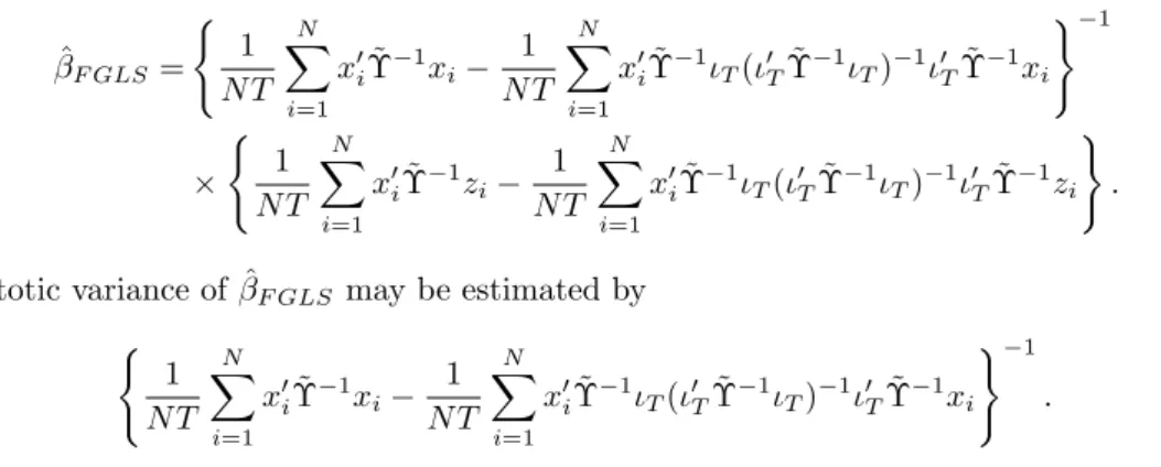
The asymptotic variance of ˆβF GLS may be estimated by
{
1
N T N ∑
i=1
x′iΥ˜−1xi−
1
N T N ∑
i=1
x′iΥ˜−1ιT(ι′TΥ˜−1ιT)−1ι′TΥ˜−1xi }−1
. (5)
We examine the properties of the feasible GLS estimator through simulations. We consider the case
in which xit is scalar. The data are generated in the following way: xit ∼ i.i.d.U[−1,1]; and yit is generated in the same way as in the experiments in Section 5. We fix the value ofβ at β = 1. We set
N = 50, T = 5,10,20,α= 0,0.5,0.9,σ2
η = 1 and σ2 is set such thatγ0 = 1. We examine the following
four estimators ofβ: the within-group estimator (“WG”); the (infeasible) GLS estimator (“GLS”); the feasible GLS estimator with ˜Υ based on ˜γk(∞)s (“FGLS”); the estimator considered by Kiefer (1980) (“KGLS”) which is the feasible GLS estimator applied to the equation transformed by the fixed effects
transformation. For each estimator, we compute the bias and the standard deviation (std). We also
give the mean of the standard error (meanse) for each estimator and the coverage probability of the 95%
confidence interval based on each estimator, where the confidence interval is constructed by the standard
formula: estimate±1.96(standard error). The standard errors are computed using formula (5.2.8) of
Hayashi (2000) for “WG”, formula (5) with Υ instead of ˜Υ for “GLS”, formula (5) for “FGLS”, and the
formula in page 199 of Kiefer (1980) for “KGLS”. We note that the standard error for “WG” allows serial
dependence but it assumes homoskedasticity conditional on the regressor.
Table 3 summarizes the results. The biases of all the estimators are negligible and the estimators
should be compared in terms of their standard deviations. Naturally, “GLS” exhibits the smallest
stan-dard deviation among the estimators compared. Both “FGLS” and “KGLS” exhibit lower stanstan-dard
deviations than does “WG”. Among these feasible GLS estimators, “FGLS” has the smallest standard
deviation and its standard deviation is similar to that of “GLS”. Moreover, the standard error and the
based on “FGLS” is close to 0.95. Although the confidence intervals based on “WG” and “GLS” have
better coverage rates than that of “FGLS” does whenα= 0.9, the confidence interval based on ”FGLS” performs better than does that based on “KGLS”. These results indicate the usefulness of “FGLS”. It has
a small standard deviation and its standard error is reliable. These results imply that the asymptotically
unbiased autocovariance estimators developed in this paper are useful for the GLS estimation of fixed
effects regression models.
[Table 3 about here]
References
Abowd, J. M. & D. Card (1989) On the covariance structure of earnings and hours changes, Econometrica
57(2), 411–445.
Alvarez, J. & M. Arellano (2003) The time series and cross-section asymptotics of dynamic panel data estimators,
Econometrica71(4), 1121–1159.
Anderson, T. W. & C. Hsiao (1981) Estimation of dynamics models with error components, Journal of the American Statistical Association76(375), 598–606.
Andrews, D. W. K. (1991) Heteroskedasticity and autocorrelation consistent covariance matrix estimation, Econo-metrica59(3), 817–858.
Arellano, M. (2003) Panel Data Econometrics, Oxford University Press.
Arellano, M. & S. Bond (1991) Some tests of specification for panel data: Monte Carlo evidence and an application to employment equations,Review of Economics Studies58, 277–297.
Baltagi, B. H. & Q. Li (1994) Estimating error component models with general MA(q) disturbances,Econometric Theory10, 396–408.
Brillinger, D. R. (1981) Time Series: Data Analysis and Theory, Holden Day. Inc.
Bun, M. J. & J. F. Kiviet (2006) The effects of dynamic feedbacks on LS and MM estimator accuracy in panel data models,Journal of Econometrics132, 409–444.
Cameron, A. C. & P. K. Trivedi (2005) Microeconometrics, Methods and Applications, Cambridge University Press.
Chamberlain, G. (1984) Panel data, in Z. Griliches and M. D. Intriligator (eds.), Handbook of Econometrics, Vol. 2, chapter 22, pp. 1247–1318. Elsevier.
den Haan, W. J. & A. T. Levin (1997) A practitioner’s guide to robust covariance matrix estimation, inG. S. Maddala and C. R. Rao (eds.),Handbook of Statistics, Vol. 15, pp. 299–342. Elsevier.
Doornik, J. A. (2007) Ox, - An Object-Oriented Matrix Programming Language, Timberlake Consultants Press, London.
Hahn, J. & G. Kuersteiner (2002) Asymptotically unbiased inference for a dynamic panel model with fixed effects when bothnandT are large,Econometrica70(4), 1639–1657.
Hahn, J. & G. Kuersteiner (2004) Bias reduction for dynamic nonlinear panel models with fixed effects, mimeo.
Hahn, J. & G. Kuersteiner (2007) Bandwidth choice for bias estimators in dynamic nonlinear panel models, mimeo.
Hansen, C. B. (2007) Generalized least squares inference in panel and multilevel models with serial correlation and fixed effects,Journal of Econometrics140, 670–694.
Hausman, J. & G. Kuersteiner (2008) Difference in difference meets generalized least squares: Higher order properties of hypotheses tests,Journal of Econometrics144, 371–391.
Hayashi, F. (2000) Econometrics, Princeton University Press.
Holtz-Eakin, D., W. Newey & H. S. Rosen (1988) Estimating vector autoregressions with panel data,Econometrica
6, 1371–1395.
Kakizawa, Y. & M. Taniguchi (1994) Asymptotic efficiency of sample covariances in a gaussian stationary process,
Journal of Time Series Analysis15, 303–311.
Kiefer, N. M. (1980) Estimation of fixed effect models for time series of cross-sections with arbitrary intertemporal covariance,Journal of Econometrics14, 195–202.
Kiviet, J. F. (1995) On bias, inconsistency, and efficiency of various estimators in dynamic panel data models,
Journal of Econometrics68, 53–78.
Lee, Y. (2008a) Bias correction in dynamic panel models under time series misspecification, mimeo.
Lee, Y. (2008b) Nonparametric estimation of dynamic panel models with fixed effects, mimeo.
Lillard, L. A. & R. J. Willis (1978) Dynamic aspects of earning mobility,Econometrica46(5), 985–1012. MaCurdy, T. E. (1982) The use of time series processes to model the error structure of earnings in a longitudinal
data analysis,Journal of Econometrics18, 83–114.
Nickell, S. (1981) Biases in dynamic models with fixed effects,Econometrica49(6), 1417–1426.
Parzen, E. (1957) Consistent estimates of the spectrum of a stationary time series, Annals of Mathematical Statistics28(2), 329–348.
Phillips, P. C. B. & H. R. Moon (1999) Linear regression limit theory for nonstationary panel data,Econometrica
67(5), 1057–1111.
Porat, B. (1987) Some asymptotic properties of the sample covariances of gaussian autoregressive moving average process,Journal of Time Series Analysis8, 205–220.
Solon, G. (1984) Estimating autocorrelations in fixed-effects models, NBER, Technical Working Paper No. 32.
A
Technical appendix
A.1
Proof of Theorem 1
Proof. We have the following decomposition: ˆ
γk =
1
N(T−k)
N X
i=1
T X
t=k+1
witwi,t−k−
1
N
N X
i=1 ( ¯wi)2
−2 k
N(T−k)
N X
i=1 ( ¯wi)2+
1
N(T−k)
N X
i=1
k X
t=1
witw¯i+
1
N(T−k)
N X
i=1
T X
t=T−k+1
witw¯i.
The first term on the right-hand side of the equation converges toγk by Lemma 1. The second and third terms
areop(1) by Lemma 2 and the fourth and fifth terms areop(1) by Lemma 3. It follows that ˆγk→pγk.
A.2
Proof of Theorem 2
Proof. We have the following decomposition:
√
N T „
ˆ
γk−γk+
1
TVT «
= √N T 1
N(T−k)
N X
i=1
T X
t=k+1
(witwi,t−k−γk)− √
N T (
1
N
N X
i=1
(¯yi−ηi)2−
1
TVT )
+2√N T k N(T−k)
N X
i=1 ( ¯wi)2+
√
N T 1 N(T−k)
N X
i=1
k X
t=1
witw¯i+ √
N T 1 N(T−k)
N X
i=1
T X
t=T−k+1
witw¯i.
The first term on the right-hand side is asymptotically normal by Lemma 1, and the second and third terms are
A.3
Proof of Theorem 4
Proof. First, we consider the bias:
E( ˜VT) = T−1
X
j=−T+1
k „
j S
« E(ˆγ+j).
Note that:
E(ˆγj+) =
T− |j|
T γj− T− |j|
T
1
TVT+BjT,
where
BjT = E 8 <
: −2 |j|
N T
N X
i=1 ( ¯wi)2+
1
N T
N X
i=1
|j| X
t=1
witw¯i+
1 N T N X i=1 T X
t=T−|j|+1
witw¯i 9 =
; .
We have
E“V˜T−VT ”
=
T−1
X
j=−T+1
ȷ k „ j S « −1 ff T − |j|
T γj
−T1VT T−1
X
j=−T+1
k „
j S
« T− |j|
T +
T−1
X
j=−T+1
k „
j S
« BjT.
As shown by Parzen (1957),Sq times the first term on the right-hand side converges to
−kqV(q). This implies
that the first term is of order O(S−q). Next, we consider the second term. Observing that V
T → V and
S−1PT−1
j=−T+1k(j/S)→
R1
−1k(x)dx, the second term is of orderO(S/T). The first term is therefore of an order larger than the second term whenSq+1/T
→0, which is satisfied whenNq+1/Tq
→0 andS2q+1/(N T)
→τ. The first term and the second term are of the same order whenSq+1/T→τ.
We consider the third term on the right-hand side. We observe that
T−1
X
j=−T+1
k „ j S « E (
2 |j|
N T
N X
i=1 ( ¯wi)2
)
=
T−1
X
j=−T+1
k „
j S
«
2|j|
T2 VT
≤ 2TS2VT T−1
X
j=−T+1
k „ j S « =O „ S2 T2 « , and that ˛ ˛ ˛ ˛ ˛ ˛
T−1
X
j=−T+1
k „ j S « E 0 @ 1 N T N X i=1
|j| X
t=1
witw¯i 1 A ˛ ˛ ˛ ˛ ˛ ˛ ≤ T−1
X
j=−T+1
k „
j S
« |j|
T2
T X
m=1
|γm| ≤
S T2
T X
m=1
|γm| T−1
X
j=−T+1
k „ j S « =O „ S2 T2 « ,
by Lemma 3. Similarly, we can show that
˛ ˛ ˛ ˛ ˛ ˛
T−1
X
j=−T+1
k „ j S « E 0 @ 1 N T N X i=1 T X
t=T−|j|+1
witw¯i 1 A ˛ ˛ ˛ ˛ ˛ ˛ =O „ S2 T2 « .
Therefore, we have
˛ ˛ ˛ ˛ ˛
T−1
X
j=−T+1
k „ j S « BjT ˛ ˛ ˛ ˛ ˛ =O „ S2 T2 « .
Therefore, we have thatE( ˜VT−VT)→0 ifS→ ∞andS/T →0. Moreover, whenSq+1/T →0,
SqE“V˜T−VT ”
and, whenSq+1/T →τ, where 0< τ <∞, we have
SqE“V˜T−VT ”
→ −kqV(q)−τ V Z
k(x)dx.
Next, we consider the variance. We note that ˆVT is the sample average across cross-sections of the long-run
variance estimator for each time series. Let
˜
VT=
1
N
N X
i=1 ˜
VT ,i,
where
˜
VT ,i≡ T−1
X
j=−T+1
k „
j S
«
1
T
T X
t=|j|+1
(yit−y¯i)(yi,t−|j|−y¯i).
Therefore, we have
var( ˜VT) =
1
Nvar( ˜VT ,i).
We verify Assumptions B, C and D in Andrews (1991), under which we can use the variance formula for ˜VT ,i
provided by Andrews (1991). Note thatθ, ˆθ andVt(θ) in Assumptions B, C and D of Andrews (1991) are ηi, ¯yi
andyit−ηi, respectively, in our case. Observing that∂(yit−ηi)/(∂ηi) =−1, we can easily verify that Assumptions
B, C and D are satisfied. Therefore, we have
N T
S var( ˜VT)→2V
2Z k(x)2dx.
This also implies thatvar( ˜VT)→0 ifS/(N T)→0.
For the first bias term and the variance term to be of the same order, we needS2q+1/(N T)
→τ. For these two terms to be of larger order than the second bias term, we needSq+1/T →0, which is equivalent toNq+1/Tq
→0 whenS=O((N T)2q1+1). Therefore, whenNq+1/Tq→0 andS2q+1/(N T)→0, the asymptotic MSE is
lim
N,T→∞ N T
S M SE( ˜VT) =k
2
q “
V(q)”2τ−1+ 2V2 Z
k2(x)dx.
On the order hand, the first and second bias terms are of the same order when Sq+1/T →τ. These terms are of larger order than the variance term when{S/(N T)}/(S/T)2→0, which is equivalent toNq+1/Tq
→ ∞when
S=O(Tq+11 ). Therefore, whenNq+1/Tq→ ∞andSq+1/T →τ, the asymptotic MSE is
lim
N,T→∞ T2
S2M SE( ˜VT) =
ȷ
−kqV(q)τ−1−V Z
k(x)dx ff2
.
A.4
Proof of Theorem 5
Proof. In this proof, we use the notation defined in the proof of Theorem 4.
First, note that the asymptotic variance of ˜VT(∞) is the same as that of ˜VT because
˜
VT(∞) = „
1 + ι
′
TKT
T−ι′
TKT «
˜
VT =
T T−ι′
TKT
˜
VT
andT /(T−ι′
TKT)→1. Therefore, we have
N T
S var{V˜T(∞)} →2V
2Z k(x)2dx.
Next, we consider the bias of ˜VT(∞):
E{V˜T(∞)−VT} = T+1
X
j=−T+1
ȷ k
„ j S
« −1
ff T− |j|
T γj
−1
TVTι ′
TKT+
ι′TKT
T−ι′
TKT T+1
X
j=−T+1
k „
j S
« T− |j|
T γj
−T1VT
ι′
TKT
T−ι′
TKT
ι′TKT+
T T−ι′
TKT T+1
X
j=−T+1
k „
j S