全文検索アジア経済研究所学術研究リポジトリ ARRIDE IDP000690 001

(1)

(2)

INSTITUTE OF DEVELOPING ECONOMIES

IDE Discussion Papers are preliminary materials circulated to stimulate discussions and critical comments

Keywords: Brexit; foreign direct investment; multinational enterprise; export-platform;

knowledge-capital model

JEL classification: F11; F12; F15; F23

Abstract

This paper explores how the British exit (Brexit) from the European Union (EU) potentially affects the United Kingdom (UK) economy and the production patterns of multinational enterprises that choose the UK as either a destination market or a gateway to the EU market. Utilizing an extended version of the knowledge-capital model, simulation analysis reveals the following points: (1) Brexit will encourage firms in both the EU and the UK to change strategies to incorporate more horizontal-type affiliates so that Brexit will not reduce inward foreign direct investment (FDI) to the UK as long as the UK is attractive as a final market; and (2) In contrast, export-platforms serving the EU market owned by firms in non-EU countries will completely withdraw by the time Brexit is completed. To cover losses from the reduction in the number of export-platforms, efforts to enhance the attractiveness of the UK as a destination market would be a solution in the short-run, while seeking new economic partnership programs with both EU and non-EU countries will work in the long-run.

IDE DISCUSSION PAPER No. 690

How Does BREXIT Affect Production Patterns of Multinational Enterprises?

Kazuhiko OYAMADA

(3)

The Institute of Developing Economies (IDE) is a semigovernmental, nonpartisan, nonprofit research institute, founded in 1958. The Institute merged with the Japan External Trade Organization (JETRO) on July 1, 1998.

The Institute conducts basic and comprehensive studies on economic and related affairs in all developing countries and regions, including Asia, the Middle East, Africa, Latin America, Oceania, and Eastern Europe.

The views expressed in this publication are those of the author(s). Publication does not imply endorsement by the Institute of Developing Economies of any of the views expressed within.

INSTITUTE OF DEVELOPING ECONOMIES (IDE), JETRO

3-2-2, WAKABA,MIHAMA-KU,CHIBA-SHI

CHIBA 261-8545, JAPAN

(4)

1

How Does BREXIT Affect Production Patterns of

Multinational Enterprises?

*

Kazuhiko OYAMADA†

February 20, 2018

Abstract

This paper explores how the British exit (Brexit) from the European Union (EU) potentially affects the United Kingdom (UK) economy and the production patterns of multinational enterprises that choose the UK as either a destination market or a gateway to the EU market. Utilizing an extended version of the knowledge-capital model that includes six types of firms and four countries grouped into market and non-market in a general equilibrium framework, simulation analysis reveals the following points: (1) Brexit will encourage firms in both the EU and the UK to change strategies to incorporate more horizontal-type affiliates so that Brexit will not reduce inward foreign direct investment (FDI) to the UK as long as the UK is attractive as a final market; and (2) In contrast, export-platforms serving the EU market owned by firms in non-EU countries will completely withdraw by the time Brexit is completed. To cover losses from the reduction in the number of export-platforms, efforts to increase horizontal FDI and enhance the attractiveness of the UK as a destination market would be a solution in the short-run, while seeking new free-trade agreements or economic partnership programs with both EU and non-EU countries will work in the long-run.

Keywords: Brexit; foreign direct investment; multinational enterprise; export-platform; knowledge-capital model

JEL Classification Numbers: F11; F12; F15; F23

* _{The author would like to express his gratitude to María Concepción Latorre (Universidad Complutense de}

Madrid) for her helpful comments and suggestions.

†_{Institute of Developing Economies, Japan External Trade Organization (IDE-JETRO), 3-2-2 Wakaba,}

(5)

2

1. Introduction

As the global economy has become increasingly interdependent, multinational enterprises (MNEs) form multilateral production networks, where production processes are subdivided into several stages and different countries have been participating in specific parts of these networks. In this environment, the United Kingdom (UK) decided to leave the European Union (EU). On March 29, 2017, the prime minister of Great Britain, Theresa May, signed a letter that will trigger the British exit from the EU (Brexit) within two years. The UK is the largest recipient of foreign direct investment (FDI) in the EU, with almost half of the FDI coming from other EU countries (Global Counsel 2015; UK Trade & Investment 2016). At a global level, the UK is the third highest recipient of FDI after the United States (US) and China (Simionescu 2016). The purpose of this paper is to explore how Brexit could affect the production patterns of MNEs that choose the UK as a destination market or as a gateway to the EU market.

While there has been extensive research on the activities of MNEs since the late 1980s, a limited number of studies have combined every operational strategy of MNEs into one model. The export-platform especially is not much discussed in the theoretical studies, even though empirical studies have shown its importance. Since the UK plays a significant role for MNEs as a gateway to the EU market, the analytical model for this study must include this type in addition to the typical horizontal- and vertical-type MNEs.

One of the most sophisticated studies to consider typical types of MNEs while including export-platforms in one consistent analytical framework was presented by Ekholm, Forslid, and Markusen (2007). Using a numerical simulation model in which two market countries and one exogenously given developing country are considered, they explored conditions under four types of firm strategy while gradually changing two types of costs, one for trading components and the other for assembling components. However, their model has only one factor of production, and the non-market country is assumed to set exogenous factor pricing in a partial equilibrium framework. Another work that nests every type of MNE in one model is presented by Ito (2013). Extending the two-region, four-country (two countries in each region) model developed by Navaretti and Venebles (2004) to include export-platform, he showed that a reduction in trade costs, either inter-regional or intra-regional, induces firms to choose the export-platform rather than other types. To enable the theoretical model to yield testable hypotheses for empirical testing, he incorporated only trade costs while abstracting away production costs.

(6)

3

production costs in a general equilibrium setting is the knowledge-capital model developed by Markusen (1997) and further extended by Zhang and Markusen (1999). Their computational model is able to verify the effects of changes in firm-type on factor prices in the countries where the MNEs are active, although export-platform is not taken into account. Oyamada (2016) extended this original model to develop a new version that includes two types of export-platform that operate in two non-market countries. This study utilizes this version of the knowledge-capital model.

The remainder of this paper is organized as follows. Section 2 illustrates the major assumptions of the extended knowledge-capital model. In Sections 3 and 4, we perform simulations and report on results that reveal which type of firms would be active under the Brexit scenario and how selected economic indicators including welfare are affected. Finally, Section 5 concludes this study.

2. The Extended Knowledge-Capital Model

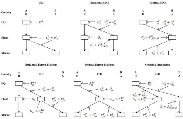
The model used in this study is a simple extension of the knowledge-capital model originally developed by Markusen (1997). This model is extended to include six types of operational strategies: national enterprises (NEs); horizontal MNEs (HMNEs); vertical MNEs (VMNEs); horizontal export-platforms (HEPs); vertical export-platforms (VEPs); and complexly integrated MNEs (CMNEs). In addition to the original assumption of two market countries in which MNE are established and there are markets for the commodity produced by these MNEs, the model also includes two non-market countries, in which the final assembly process of multinational production may take place while the finished products are exported rather than sold locally.

(7)

4

integration CI share identical technologies and productivity. In contrast, Z is the regular good produced by the non-MNE with a constant-returns-to-scale technology so that its market is perfectly competitive. Z is produced in every country r, and sold on the international market as a perfect substitute.

In the IRTS sector, two types of fixed costs (F and G) are required to start operating a firm. While G, measured in units of unskilled labor L, is needed to set up an assembly plant in country r (country specific), F, measured in units of skilled labor K, is required to establish a firm and its local subsidiary to operate on a trade-link between the home and a foreign country (firm-type/trade-link specific). There are trade costs (transportation costs and import tariffs) for the international transport of X and Y, which are specific to each trade link. We assume that unskilled labor L in the exporting country is used for transportation. On the other hand, it is assumed for simplicity that shipping Z does not generate any cost.

In this environment, there are two groups of firms producing Y. One is established and headquartered in country A and the other in B (country i). The markets for Y are limited to countries A and B (country j). Good Y is produced in two stages with IRTS technology by imperfectly competitive firms. In the first stage, each firm produces its components (the intermediate good) X only in its home country using skilled labor K. In the second stage, a firm sends its components to domestic and/or foreign subsidiaries to finalize the production of Y there, assembling components X using locally hired unskilled labor L. This assembly process can take place in any country r. If the assembly is taking place in a non-market country w, all of the final products are exported to one or both of the market countries j. If it is performed in the home country i, the products are sold domestically and/or exported to a foreign market j. If it takes place in a foreign market country i, the products are sold locally and/or exported back to the home market j.

(8)

5

Type-N: NEs that maintain a single plant with headquarters in country i. This type of firms produces both components X and final products Y in country i. A fraction of the production of product Y may or may not be exported to country j.

Type-H: HMNEs that maintain plants in both market countries, with headquarters in country i. This type of firm produces components X in country i, some of which are shipped to an assembly plant in country j. The final products Y are produced in both market countries. No fraction of product Y may be exported.

Type-V: VMNEs that maintain a single plant in the foreign market country j, with headquarters in country i. This type of firm produces components X in country i, which are then shipped to the assembly plant in country j. A fraction of the products Y may or may not be exported back to the home market in country i.

Type-EH: HEPs that maintain a plant in one of the non-market countries w, in addition to a plant and headquarters in home country i. This type of firms produces components X in country i, some of which are shipped to an assembly plant in country w. All of the final product Y produced in country w is exported to the foreign market in country j, while products produced in the home country are sold domestically.

Type-EV: VEPs that maintain a single plant in one of the non-market countries w, with headquarters in country i. This type of firm produces component X in country i, which is then shipped to the assembly plant in country w. All of the final product Y is exported to both of the market countries j.

Type-CI: CMNEs that maintain plants both in one of the non-market countries w and in the foreign market country j, with headquarters in country i. This type of firm produces component X in country i, which is then shipped to the assembly plant in countries w and j. All of the final product Y produced in country w is exported back to the home market in country i, while that produced in the foreign market country is sold locally.

(9)

6

group. The factor endowments for the group not being focused on are kept identical for the two countries in the group to avoid complexities in interpreting the results. Then, a box diagram à la Edgeworth box is drawn placing the total skilled labor endowment for the

focused group on one axis and the total unskilled labor endowment on another axis to capture the regime, welfare level, factor prices, and so on in each cell corresponding to the relative factor endowments of the two countries. The full set of the system of equations and inequalities that solves for an equilibrium is presented in Oyamada (2016).

Figure 1: Six Types of Production Patterns

Assumptions on the levels of fixed costs and their relationships play a crucial role in the predictions of the model. We made the following four assumptions on the firm-type/trade-link specific fixed cost F for a firm established in country A:

, (1)

, (2)

, (3)

(10)

7

. (4)

The case for a firm established in country B is the same. Relation (1) is based on the joint-input characteristic of knowledge-based services that enables simultaneous use in multiple production facilities. The cost for an additional plant may be reduced. Relation (2) is related to the headquarter cost. First, a type-H firm is more expensive compared with a type-N firm because additional skilled labor is required at headquarters for managerial and coordination activities. Second, the additional cost of managerial and coordination activities for the operation of a local subsidiary might be higher in a non-market country (type-EH and type-CI) than in a market country (type-H). A similar relationship applies to type-V and type-EV firms. Third, a type-N firm is costly compared to a type-V or type-EV firm because the latter may hire local skilled labor to train unskilled labor in the host country. Relation (3) is related to the local affiliate cost. In non-market countries, cheaper skilled labor is available. Relation (4) is related to the total cost. Type-V and type-EV firms are less costly compared to type-H and type-EH firms because the former has only one assembly plant in a non-market country and additional payment for managerial coordination activities is therefore not required. Among type-H and type-EH firms, we assume that operating an assembly plant is more costly in a market country than in a non-market country. A similar relationship applies to type-V and type-EV firms. The most costly firm is the type-CI because this type operates its headquarters and two assembly plants in three different countries. Relation (4) also implies that technology transfer incurs some amount of cost so that fragmentation is not perfect.

One point to note is that we presume the plant-level production of the type-Y good is less skilled-labor intensive than that of the type-Z, which represents the composite of all kinds of commodities, unlike the original theory (Carr, Markusen, and Maskus 2001:694; Markusen 2002:133). Based on the Global Trade Analysis Project (GTAP) 9A Data Base for 2011 (Hertel 1997), shares of skilled-labor in the total labor inputs with respect to the manufacturing sector, primary industries, and services are 37.837%, 56.795%, and 48.707%, respectively, in the 24 countries in which the world's top 100 non-financial MNEs for 2015 (UNCTAD 2016) are established, and the overall production in the rest of the world.1_{The countries with the top 100 investors can be regarded as the market}

1_{The 24 countries are: Australia, China, Hong Kong, Japan, Korea, Taiwan, Malaysia, United States,}

(11)

8

countries in this study, while the countries without are the non-market countries. Assuming that MNEs mainly reside in the manufacturing sector, we can then stipulate the skilled-labor intensity of activities as:

(Headquarters Only)

(Integrated Production of Type-Y) (Production of Type-Z)

(Plant Only).

This assumption on factor-intensity significantly affects the simulation results we will see later. While MNEs are considered in many cases as more skilled-labor intensive than local firms in developing countries, we suspect that the hypothesis holds only within the same industrial category.

Various operational patterns appear under different characteristics of the countries. When two market countries are similar in both size and relative endowment, type-H firms established in both market countries prevail. If the market countries differ in size while being similar in relative endowment, type-N firms established in the country with abundant factors dominate the production and occupy both markets. When the price of unskilled labor in a market country becomes cheaper, foreign type-H firms become active. If the price of unskilled labor becomes extremely high, firms established in the country move to other market countries as type-V firms. In this environment, MNEs never establish plants in non-market countries but instead go straight to market countries as type-N, type-H, or type-V firms if non-market countries are similar in relative endowment. The reason for this is that there is no substantial difference between relative factor prices among the non-market countries. On the other hand, type-EV firms become active if cheaper unskilled labor is available in either of the non-market countries. For instance, type-EV firms from both countries A and B operate in C when unskilled labor is relatively abundant in country C. Type-EH firms tend to arise in non-market countries where both low-trade-cost access to the final market and cheap unskilled labor is available. One example of this is the construction of factories in a free trade area to serve the markets of other members of the free trade agreement (FTA) while avoiding import tariffs. Type-CI firms emerge under a particular condition in which a market country and a non-market country liberalize trade in an environment in which the transportation cost of components is low while the cost of finished products concerning the trade-link between market countries is high. An example of a low transportation cost of components is the use of the internet to send blue prints from

(12)

9 headquarters to a local affiliate.

3. The Effects of BREXIT on FDI in the UK as a Destination Market

We now examine the potential effects of Brexit when the UK is considered as a destination market. As mentioned in Section 1, almost half of the inward FDI to the UK was from other EU countries. This kind of FDI from the EU area may not be for the purpose of building export-platforms but solely to serve the UK market. Therefore, the operational strategy of MNEs will be type-H or type-V. Suppose two market countries A and B are one of the EU countries, which is investing to the UK, and the UK, respectively.

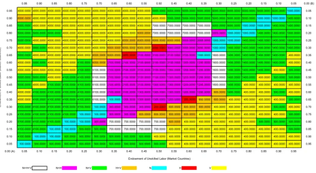
Figure 2: Operational Patterns when Import Tariff Is Low (Market Countries)

Then, let us examine Figure 2, a box diagram for the case when relative factor endowments for the two market countries are changed given the absolute levels of total endowments. To simulate the situation when the UK is still a member of the EU, import tariff rates levied on both the component X and the final product Y traded between countries A and B are set to zero. This will be the base case for comparison with the results obtained when a set of parameters or exogenous variables are changed. The vertical axis corresponds to the total endowment of skilled labor for the two market countries, and the horizontal axis to that of unskilled labor. The division of the factor endowments between

0.95 0.90 0.85 0.80 0.75 0.70 0.65 0.60 0.55 0.50 0.45 0.40 0.35 0.30 0.25 0.20 0.15 0.10 0.05 0.00 (B)

0.95 4000.0000 4000.0000 4000.0000 4000.0000 4000.0000 4000.0000 4000.0000 4000.0000 4000.0000 5000.0000 5000.0000 5000.0000 5000.0000 5000.0000 5000.0000 5000.0000 5000.0000 5000.0000 1000.0000 0.05

0.90 6000.0000 4000.0000 4000.0000 4000.0000 4000.0000 4000.0000 4000.0000 4000.0000 4000.0000 4000.0000 5000.0000 5000.0000 5000.0000 5000.0000 5000.0000 5000.0000 1000.0000 1000.0000 1400.0000 0.10

0.85 5000.0000 4000.0000 4000.0000 4000.0000 4000.0000 4000.0000 4000.0000 4000.0000 4000.0000 7000.0000 7000.0000 7000.0000 7000.0000 5000.0000 5000.0000 1000.0000 1000.0000 1400.0000 1400.0000 0.15

0.80 5000.0000 5000.0000 5000.0000 4000.0000 4000.0000 4000.0000 4000.0000 4000.0000 6000.0000 7000.0000 7000.0000 7000.0000 7000.0000 3000.0000 1000.0000 1000.0000 1400.0000 1400.0000 1500.0000 0.20

0.75 5000.0000 4000.0000 4000.0000 4000.0000 4000.0000 4000.0000 4000.0000 6000.0000 6000.0000 6000.0000 6000.0000 3000.0000 3000.0000 1000.0000 1000.0000 1400.0000 1400.0000 1400.0000 1500.0000 0.25

0.70 4000.0000 5000.0000 4000.0000 4000.0000 4000.0000 4000.0000 6000.0000 6000.0000 6000.0000 2000.0000 3000.0000 3000.0000 3000.0000 1000.0000 1400.0000 1400.0000 1400.0000 1400.0000 1400.0000 0.30

0.65 5000.0000 4000.0000 4000.0000 4000.0000 4000.0000 6000.0000 6000.0000 2000.0000 2100.0000 3100.0000 3100.0000 3100.0000 1000.0000 1600.0000 1400.0000 1400.0000 1400.0000 1400.0000 400.0000 0.35

0.60 4000.0000 5000.0000 4000.0000 4000.0000 4100.0000 6000.0000 2100.0000 2100.0000 3100.0000 3100.0000 3100.0000 1300.0000 1200.0000 1600.0000 1400.0000 1400.0000 1400.0000 1400.0000 400.0000 0.40

0.55 4000.0000 4000.0000 4000.0000 4000.0000 4100.0000 6100.0000 2100.0000 2100.0000 3100.0000 3100.0000 1300.0000 1200.0000 1200.0000 1600.0000 1400.0000 1400.0000 1400.0000 400.0000 500.0000 0.45

0.50 5000.0000 5000.0000 4000.0000 4100.0000 4100.0000 6100.0000 2100.0000 2100.0000 3100.0000 1100.0000 1300.0000 1200.0000 1200.0000 1600.0000 1400.0000 1400.0000 400.0000 500.0000 500.0000 0.50

0.45 5000.0000 4000.0000 4100.0000 4100.0000 4100.0000 6100.0000 2100.0000 2100.0000 3100.0000 1300.0000 1300.0000 1200.0000 1200.0000 1600.0000 1400.0000 400.0000 400.0000 400.0000 400.0000 0.55

0.40 4000.0000 4100.0000 4100.0000 4100.0000 4100.0000 6100.0000 2100.0000 3100.0000 1300.0000 1300.0000 1300.0000 1200.0000 1200.0000 600.0000 1400.0000 400.0000 400.0000 500.0000 400.0000 0.60

0.35 4000.0000 4100.0000 4100.0000 4100.0000 4100.0000 6100.0000 100.0000 1300.0000 1300.0000 1300.0000 1200.0000 200.0000 600.0000 600.0000 400.0000 400.0000 400.0000 400.0000 500.0000 0.65

0.30 4100.0000 4100.0000 4100.0000 4100.0000 4100.0000 100.0000 300.0000 300.0000 300.0000 200.0000 600.0000 600.0000 600.0000 400.0000 400.0000 400.0000 400.0000 500.0000 400.0000 0.70

0.25 4100.0000 4100.0000 4100.0000 4100.0000 100.0000 100.0000 300.0000 300.0000 600.0000 600.0000 600.0000 600.0000 400.0000 400.0000 400.0000 400.0000 400.0000 400.0000 500.0000 0.75

0.20 5100.0000 4100.0000 4100.0000 100.0000 100.0000 300.0000 700.0000 700.0000 700.0000 700.0000 600.0000 400.0000 400.0000 400.0000 400.0000 400.0000 500.0000 500.0000 500.0000 0.80

0.15 4100.0000 4100.0000 100.0000 100.0000 500.0000 500.0000 700.0000 700.0000 700.0000 700.0000 400.0000 400.0000 400.0000 400.0000 400.0000 400.0000 400.0000 400.0000 500.0000 0.85

0.10 4100.0000 100.0000 100.0000 500.0000 500.0000 500.0000 500.0000 500.0000 500.0000 400.0000 400.0000 400.0000 400.0000 400.0000 400.0000 400.0000 400.0000 400.0000 400.0000 0.90

0.05 100.0000 500.0000 500.0000 500.0000 500.0000 500.0000 500.0000 500.0000 500.0000 500.0000 400.0000 400.0000 400.0000 400.0000 400.0000 400.0000 400.0000 400.0000 400.0000 0.95

0.00 (A) 0.05 0.10 0.15 0.20 0.25 0.30 0.35 0.40 0.45 0.50 0.55 0.60 0.65 0.70 0.75 0.80 0.85 0.90 0.95

N+H+V N+H N+V H+V N H V

En do w m en t o f Ski lle d L ab or (M ar ke t C ou ntr ie s)

(13)

10

the two countries is shown with country A measured from the southwest corner and country B measured from the northeast corner. The model is repeatedly solved for each cell 361 (19 19) times, altering the distribution of factor endowments. Each cell represents an equilibrium regime and the number inside shows which type of firm is active in the regime. The regime number is defined as:

,

where

if type-N firms established in country A are active, otherwise 0; if type-N firms established in country B are active, otherwise 0;

if type-H firms established in country A are active, otherwise 0; if type-H firms established in country B are active, otherwise 0; 4 if type-V firms established in country A are active, otherwise 0; 4 if type-V firms established in country B are active, otherwise 0;

if type-EH firms established in country A operating in country C are active, otherwise 0;

if type-EH firms established in country A operating in country D are active, otherwise 0;

if type-EH firms established in country B operating in country C are active, otherwise 0;

if type-EH firms established in country B operating in country D are active, otherwise 0;

. if type-EV firms established in country A operating in country C are active, otherwise 0;

. if type-EV firms established in country A operating in country D are active, otherwise 0;

. if type-EV firms established in country B operating in country C are active, otherwise 0;

. if type-EV firms established in country B operating in country D are active, otherwise 0;

. if type-CI firms established in country A operating in country C are active, otherwise 0;

. if type-CI firms established in country A operating in country D are active, otherwise 0;

(14)

11 are active, otherwise 0; and

. if type-CI firms established in country B operating in country D are active, otherwise 0.

The situation in which firms established in one of the EU countries (country A) are investing in the UK as type-H or type-V is expressed with the number 2000, 3000, 4000, 5000, 6000, or 7000. The cells with those numbers show up in the northwestern half of Figure 2. Those firms are investing in the UK for the purpose of hiring relatively cheap unskilled labor compared with their home country.

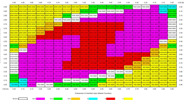
Figure 3: Operational Patterns when Import Tariff Is High (Market Countries)

In this environment, Brexit can be simulated through increases in import tariff rates on the trade between countries A and B. This is depicted by Figure 3. Notice that the cells with 2000 and 3000 increase, leaving the cells with 4000 and 5000 around the northwest corner unchanged. This implies that Brexit will not reduce FDI but increase type-H MNEs. Outward FDI from the UK to the EU also increases (numbered 200). Thus, Brexit may encourage firms in the EU to change their strategy from type-V to type-H, and firms in the UK from type-N to type-H. As long as the UK is attractive as a final market, Brexit will not reduce inward FDI to the UK but rather increase type-H activities between the UK and EU. It also works for the non-EU partners. If demand for consumption in the UK continues, firms from any country will continue investing as type-H to serve the UK market, regardless of Brexit.

0.95 0.90 0.85 0.80 0.75 0.70 0.65 0.60 0.55 0.50 0.45 0.40 0.35 0.30 0.25 0.20 0.15 0.10 0.05 0.00 (B)

0.95 4000.0000 4000.0000 4000.0000 4000.0000 4000.0000 4000.0000 4000.0000 4000.0000 4000.0000 5000.0000 5000.0000 5000.0000 5000.0000 5000.0000 7000.0000 7000.0000 3000.0000 1000.0000 1000.0000 0.05

0.90 4000.0000 4000.0000 4000.0000 4000.0000 4000.0000 4000.0000 4000.0000 4000.0000 5000.0000 5000.0000 7000.0000 7000.0000 7000.0000 3000.0000 3000.0000 3000.0000 3000.0000 1000.0000 1400.0000 0.10

0.85 4000.0000 4000.0000 4000.0000 4000.0000 4000.0000 4000.0000 5000.0000 7000.0000 7000.0000 7000.0000 3000.0000 3000.0000 3000.0000 3000.0000 3000.0000 3000.0000 3200.0000 1200.0000 1400.0000 0.15

0.80 4000.0000 4000.0000 4000.0000 4000.0000 4000.0000 7000.0000 7000.0000 7000.0000 3000.0000 3000.0000 3000.0000 3000.0000 3000.0000 3000.0000 3000.0000 3200.0000 3200.0000 1200.0000 1600.0000 0.20

0.75 4000.0000 4000.0000 4000.0000 4000.0000 6000.0000 6000.0000 2000.0000 2000.0000 2000.0000 2000.0000 2000.0000 2000.0000 2000.0000 3200.0000 3200.0000 3200.0000 3200.0000 1200.0000 1600.0000 0.25

0.70 4000.0000 4000.0000 4000.0000 6000.0000 6000.0000 2000.0000 2000.0000 2000.0000 2000.0000 2000.0000 2000.0000 2200.0000 2200.0000 3200.0000 3200.0000 3200.0000 3200.0000 1200.0000 1600.0000 0.30

0.65 4000.0000 4000.0000 4000.0000 6000.0000 2000.0000 2000.0000 2000.0000 2000.0000 2200.0000 2200.0000 2200.0000 2200.0000 3200.0000 3200.0000 3200.0000 3200.0000 1200.0000 1200.0000 1600.0000 0.35

0.60 4000.0000 4000.0000 6000.0000 2000.0000 2000.0000 2000.0000 2100.0000 2300.0000 2200.0000 2200.0000 2200.0000 2200.0000 3200.0000 3200.0000 3200.0000 3200.0000 1200.0000 1200.0000 1600.0000 0.40

0.55 4000.0000 4000.0000 6000.0000 2100.0000 2100.0000 2100.0000 2300.0000 2300.0000 2200.0000 2200.0000 2200.0000 2200.0000 3200.0000 3200.0000 3200.0000 1200.0000 1200.0000 1600.0000 400.0000 0.45

0.50 5000.0000 6000.0000 2100.0000 2100.0000 2100.0000 2300.0000 2300.0000 2300.0000 2200.0000 2200.0000 2200.0000 3200.0000 3200.0000 3200.0000 1200.0000 1200.0000 1200.0000 600.0000 500.0000 0.50

0.45 4000.0000 6100.0000 2100.0000 2100.0000 2300.0000 2300.0000 2300.0000 2200.0000 2200.0000 2200.0000 2200.0000 3200.0000 3200.0000 1200.0000 1200.0000 1200.0000 600.0000 400.0000 400.0000 0.55

0.40 6100.0000 2100.0000 2100.0000 2300.0000 2300.0000 2300.0000 2300.0000 2200.0000 2200.0000 2200.0000 2200.0000 3200.0000 1200.0000 200.0000 200.0000 200.0000 600.0000 400.0000 400.0000 0.60

0.35 6100.0000 2100.0000 2100.0000 2300.0000 2300.0000 2300.0000 2300.0000 2200.0000 2200.0000 2200.0000 2200.0000 200.0000 200.0000 200.0000 200.0000 600.0000 400.0000 400.0000 400.0000 0.65

0.30 6100.0000 2100.0000 2300.0000 2300.0000 2300.0000 2300.0000 2200.0000 2200.0000 200.0000 200.0000 200.0000 200.0000 200.0000 200.0000 600.0000 600.0000 400.0000 400.0000 400.0000 0.70

0.25 6100.0000 2100.0000 2300.0000 2300.0000 2300.0000 2300.0000 200.0000 200.0000 200.0000 200.0000 200.0000 200.0000 200.0000 600.0000 600.0000 400.0000 400.0000 400.0000 400.0000 0.75

0.20 6100.0000 2100.0000 2300.0000 2300.0000 300.0000 300.0000 300.0000 300.0000 300.0000 300.0000 300.0000 700.0000 700.0000 700.0000 400.0000 400.0000 400.0000 400.0000 400.0000 0.80

0.15 4100.0000 2100.0000 2300.0000 300.0000 300.0000 300.0000 300.0000 300.0000 300.0000 700.0000 700.0000 700.0000 500.0000 400.0000 400.0000 400.0000 400.0000 400.0000 400.0000 0.85

0.10 4100.0000 100.0000 300.0000 300.0000 300.0000 300.0000 700.0000 700.0000 700.0000 500.0000 500.0000 400.0000 400.0000 400.0000 400.0000 400.0000 400.0000 400.0000 400.0000 0.90

0.05 100.0000 100.0000 300.0000 700.0000 700.0000 500.0000 500.0000 500.0000 500.0000 500.0000 400.0000 400.0000 400.0000 400.0000 400.0000 400.0000 400.0000 400.0000 400.0000 0.95

0.00 (A) 0.05 0.10 0.15 0.20 0.25 0.30 0.35 0.40 0.45 0.50 0.55 0.60 0.65 0.70 0.75 0.80 0.85 0.90 0.95

N+H+V N+H N+V H+V N H V

En do w m en t o f Ski lle d L ab or (M ar ke t C ou ntr ie s)

(15)

12

(16)

13

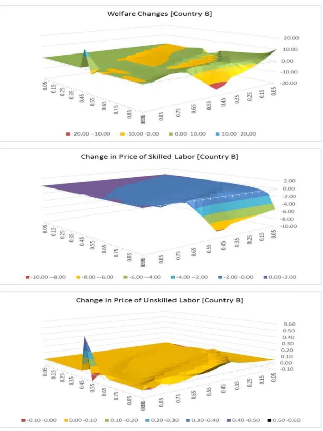
Figure 5: Effects of Reducing Fixed Cost F (Country B)

(17)

14

the price of unskilled labor, respectively in country B (the UK). In the panels, we are standing on the origin for country B, which corresponds to the northeast corner of the previously shown box diagrams.

Unexpectedly, the UK will be better off after Brexit if the country is moderately smaller than the partner country. Since the UK likely has a smaller relative endowment of skilled or unskilled labor compared with the EU or other market countries, the peaks around the left and the right corners are ignored at this time. The improvement in welfare is brought about by the increase in disposable income from the appreciation of the price of unskilled labor. The increases in import tariff rates after Brexit encourage firms to adopt a horizontal strategy so that demand for local unskilled labor increases and pushes its price up if the inward FDI mainly expands, or demand for the local skilled labor increases if the outward FDI increases compared to inward FDI, under the present assumption of skilled-labor intensity among activities. In general, income increases/decreases due to Brexit when the UK is relatively smaller/larger than the partner.

In cases when the depreciation of the price of unskilled labor causes a problem, efforts such as reducing the firm-type/trade-link specific fixed cost F, improving or developing infrastructures, may help. Since the fixed cost F is the cost of the managerial and coordination activities for the operation of a local affiliate, which requires skilled labor, the reduction of this cost saves the factor input so that its price depreciates. In turn, the cost reduction brings in inward FDI that hires more unskilled labor. Consequently, disposable income increases through the appreciation of the price of unskilled labor, improving welfare. Figure 5 captures this process.

4. The Effects of BREXIT on FDI in the UK as a Gateway to the EU

Market

In this section, we examine the potential effects of Brexit when the UK is a gateway to the EU market. This type of FDI is included in inward FDI to the UK from non-EU countries that is not for the purpose of serving the UK market. The operational strategy of MNEs will therefore be type-EH or type-EV. Suppose two non-market countries C and D are the UK and a non-EU country adjacent to the EU market, respectively. The market countries A and B are assumed to be an EU country and a non-EU market country, such as the US, Japan, or China.

(18)

15

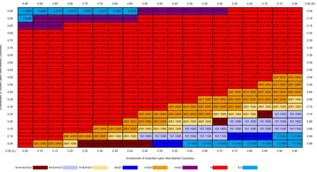
non-market countries are changed given the absolute levels of total endowments. To simulate the situation when the UK is still a member of the EU, import tariff rates levied on both the component X and the final product Y traded between countries A and C are set to zero. Analogous to the case of market countries, the division of the factor endowments between the two non-market countries is shown with country C measured from the southwest corner and country D measured from the northeast corner. The situation wherein firms established in one of the non-EU market countries (country B) are investing in the UK as type-EH or type-EV is expressed with the number 1 or 0.01. While the cells with those numbers show up around the southeastern corner of Figure 6, the type-EV may not be the case this time because it is not realistic to treat the UK as an extremely unskilled-labor-abundant country. We therefore focus on the orange colored area along the neighborhood of the southwest-northeast diagonal.

Figure 6: Operational Patterns when Import Tariff between Countries A and C Is Low (Non-Market Countries)

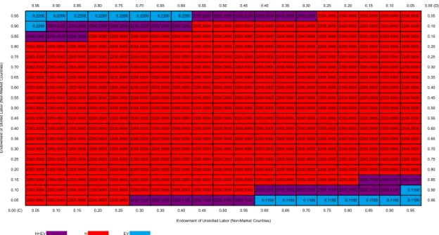
In this environment, Brexit is simulated through increases in import tariff rates on the trade between countries A and C. This is depicted in Figure 7. Notice that the cells with 1 completely disappear. This implies that the UK is no longer attractive as a gateway to the EU market and MNEs established in country B will change their strategy to build affiliate plants in the EU countries while withdrawing export-platforms from the UK. Thus, Brexit may encourage firms to go straight to the destination market as type-H.

0.95 0.90 0.85 0.80 0.75 0.70 0.65 0.60 0.55 0.50 0.45 0.40 0.35 0.30 0.25 0.20 0.15 0.10 0.05 0.00 (D)

0.95 0.2200 0.2200 0.2200 0.2200 0.2200 0.2200 0.2200 0.2200 2200.2200 2200.2200 2200.2200 2200.2200 2200.2200 2200.2200 2200.0000 2200.0000 2200.0000 2200.0000 2200.0000 0.05

0.90 0.2200 2200.2200 2200.2200 2200.2200 2200.2200 2200.2200 2200.2200 2200.2200 2200.0000 2200.0000 2200.0000 2200.0000 2200.0000 2200.0000 2200.0000 2200.0000 2200.0000 2200.0000 2200.0000 0.10

0.85 2200.2200 2200.2200 2200.2200 2200.0000 2200.0000 2200.0000 2200.0000 2200.0000 2200.0000 2200.0000 2200.0000 2200.0000 2200.0000 2200.0000 2200.0000 2200.0000 2200.0000 2200.0000 2200.0000 0.15

0.80 2200.0000 2200.0000 2200.0000 2200.0000 2200.0000 2200.0000 2200.0000 2200.0000 2200.0000 2200.0000 2200.0000 2200.0000 2200.0000 2200.0000 2200.0000 2200.0000 2200.0000 2200.0000 2200.0000 0.20

0.75 2200.0000 2200.0000 2200.0000 2200.0000 2200.0000 2200.0000 2200.0000 2200.0000 2200.0000 2200.0000 2200.0000 2200.0000 2200.0000 2200.0000 2200.0000 2200.0000 2200.0000 2200.0000 2200.0000 0.25

0.70 2200.0000 2200.0000 2200.0000 2200.0000 2200.0000 2200.0000 2200.0000 2200.0000 2200.0000 2200.0000 2200.0000 2200.0000 2200.0000 2200.0000 2200.0000 2200.0000 2200.0000 2200.0000 2200.0000 0.30

0.65 2200.0000 2200.0000 2200.0000 2200.0000 2200.0000 2200.0000 2200.0000 2200.0000 2200.0000 2200.0000 2200.0000 2200.0000 2200.0000 2200.0000 2200.0000 2200.0000 2200.0000 2200.0000 2200.0000 0.35

0.60 2200.0000 2200.0000 2200.0000 2200.0000 2200.0000 2200.0000 2200.0000 2200.0000 2200.0000 2200.0000 2200.0000 2200.0000 2200.0000 2200.0000 2200.0000 2200.0000 2200.0000 2200.0000 2200.0000 0.40

0.55 2200.0000 2200.0000 2200.0000 2200.0000 2200.0000 2200.0000 2200.0000 2200.0000 2200.0000 2200.0000 2200.0000 2200.0000 2200.0000 2200.0000 2200.0000 2200.0000 2200.0000 2200.0000 2200.0000 0.45

0.50 2200.0000 2200.0000 2200.0000 2200.0000 2200.0000 2200.0000 2200.0000 2200.0000 2200.0000 2200.0000 2200.0000 2200.0000 2200.0000 2200.0000 2200.0000 2200.0000 2200.0000 2201.0000 2201.0000 0.50

0.45 2200.0000 2200.0000 2200.0000 2200.0000 2200.0000 2200.0000 2200.0000 2200.0000 2200.0000 2200.0000 2200.0000 2200.0000 2200.0000 2200.0000 2200.0000 2200.0000 2201.0000 2201.0000 2001.0000 0.55

0.40 2200.0000 2200.0000 2200.0000 2200.0000 2200.0000 2200.0000 2200.0000 2200.0000 2200.0000 2200.0000 2200.0000 2200.0000 2200.0000 2200.0000 2201.0000 2201.0000 2001.0000 2001.0000 2001.0000 0.60

0.35 2200.0000 2200.0000 2200.0000 2200.0000 2200.0000 2200.0000 2200.0000 2200.0000 2200.0000 2200.0000 2200.0000 2200.0000 2201.0000 2201.0000 2001.0000 2001.0000 2001.0000 2001.0000 2001.1000 0.65

0.30 2200.0000 2200.0000 2200.0000 2200.0000 2200.0000 2200.0000 2200.0000 2200.0000 2200.0000 2200.0000 2201.0000 2201.0000 2001.0000 2001.0000 2001.0000 2001.1000 2001.1000 2001.1000 2001.1000 0.70

0.25 2200.0000 2200.0000 2200.0000 2200.0000 2200.0000 2200.0000 2200.0000 2200.0000 2201.0000 2201.0000 2201.0000 2001.0000 2001.0000 2001.1000 2001.1000 2001.1000 2101.1000 101.1000 101.1000 0.75

0.20 2200.0000 2200.0000 2200.0000 2200.0000 2200.0000 2200.0000 2200.0000 2201.0000 2201.0000 2001.0000 2001.1000 2001.1000 2001.1000 2101.1000 101.1000 101.1000 101.1000 101.1000 101.1000 0.80

0.15 2200.0000 2200.0000 2200.0000 2200.0000 2200.0000 2201.0000 2201.0000 2001.0000 2001.1000 2001.1000 2001.1000 101.1000 101.1000 101.1000 101.1000 101.1000 101.1000 101.1100 101.1100 0.85

0.10 2200.0000 2200.0000 2200.0000 2201.0000 2201.0000 2001.0000 2001.1000 2001.1000 101.1000 101.1000 101.1000 101.1000 101.1100 101.1100 100.1100 100.1100 100.1100 0.1100 0.1100 0.90

0.05 2200.0000 2201.0000 2201.0000 2001.1000 2101.1000 2301.1000 301.1000 301.1100 301.1100 100.1100 100.1100 0.1100 0.1100 0.1100 0.1100 0.1100 0.1100 0.1100 0.1100 0.95

0.00 (C) 0.05 0.10 0.15 0.20 0.25 0.30 0.35 0.40 0.45 0.50 0.55 0.60 0.65 0.70 0.75 0.80 0.85 0.90 0.95

N+H+EH+EV N+EH+EV H+EH+EV N+EV H+EH H+EV H EV

En do w m en t o f Ski lle d L ab or (N on -M ar ke t C ou ntr ie s)

(19)

16

Figure 7: Operational Patterns when Import Tariff between Countries A and C Is Raised (Non-Market Countries)

The effects of raising import tariff rates levied on the trade between countries A and C on the welfare and the prices of skilled and unskilled labor in country C (the UK) are shown in Figure 8. In the panels, we are standing on the origin for country C, which corresponds to the southwest corner of the box in Figure 6 or 7. Ignoring the area next to the right corner where unskilled labor is extremely abundant, country C will be worse off. After the complete withdrawal of the type-EH export-platform from country C, demand for unskilled labor falls such that the price of the factor depreciates, thereby lowering disposable income. Although the relative price of skilled labor appreciates, it is not enough to offset the reduction in the income from unskilled labor.

Since the level of trade costs plays a significant and crucial role in the firms' decision making when deciding whether to setup export-platforms in a country adjacent to the target market, long distances between the firms' home country and the target country can cause the trade cost burden to become relatively heavy when direct access is committed. The cost saving policy of reducing the firm-type/trade-link specific fixed cost F will therefore not help in this case. To cover the loss from the reduction in the number of export-platforms serving for the EU market after Brexit, efforts to increase horizontal FDI and increase its attractiveness as a destination market would be a solution in the short-run. Seeking new free trade agreements or economic partnership programs with both EU and non-EU countries