Optimal Monetary Policy at the Zero Interest Rate Bound:
The Case of Endogenous Capital Formation
Tamon Takamura
yTsutomu Watanabe
zTakeshi Kudo
xFirst Draft: December 2005
This Version: April 2012
Abstract
This paper examines optimal monetary policy at the zero interest rate bound in a sticky price economy with variable capital. We conduct a numerical comparison between the optimal discretionary and the optimal commitment policy in response to an adverse aggregate technology shock that brings about a negative natural rate of interest. We show that, when the shock is unanticipated, the outcome under discretion is inferior to that under commitment, as shown by previous studies with …xed capital models. However, when a shock is anticipated in advance, preemptive easing by a discretionary central bank stimulates investment and accelerates capital accumulation, thereby contributing to an increase in production capacity in post-liquidity-trap periods. In this sense, the suboptimality of discretion shrinks in an economy with variable capital. Under reasonable parameter settings, this “capital channel” makes up for the central bank’s inability to make a commitment about the future course of monetary policy at the zero interest rate bound.
JEL Classi…cation Numbers: E31; E52; E58; E61
Keywords: De‡ation; zero lower bound for interest rates; liquidity trap; endogenous capital formation
We would like to thank Kosuke Aoki, Ippei Fujiwara, Shigenori Shiratsuka, and seminar participants at Hitotsubashi University, Osaka University, the Bank of Japan, and Bank Indonesia for useful comments on an earlier version of this paper. We also appreciate detailed and extremely helpful comments from the editor, Carl Walsh, and three anonymous referees. This research forms part of a project on "Understanding In‡ation Dynamics of the Japanese Economy" funded by a JSPS Grant-in-Aid for Creative Scienti…c Research (18GS0101).
yCorrespondence: Tamon Takamura, Department of Economics, The Ohio State University, E-mail: [email protected].
zGraduate School of Economics, University of Tokyo, E-mail: [email protected]
1 Introduction
Recent papers on optimal monetary policy at the zero interest rate bound start their analysis by considering a situation in which the natural rate of interest falls below zero (e.g., Jung et al. 2005; Eggertsson and Woodford 2003a, b; Adam and Billi 2006, 2007; Nakov 2008). An important assumption commonly adopted in these papers is that the capital stock is …xed over time and therefore the natural rate of interest is exogenously given. This is a convenient assumption to simplify analysis, but it involves the risk that some important aspects of optimal policy responses to a negative natural rate of interest may be overlooked. In particular, it may potentially be inappropriate to ignore the consequences of monetary easing on capital accumulation as well as the e¤ect of changes in the capital stock on the natural rate of interest. In this paper, we depart from previous studies by employing a model with variable capital, in which the natural rate of interest is endogenously determined, and examine the optimal monetary policy response to adverse shocks that bring about a decline of the natural rate of interest to a negative level.
To illustrate the role of an endogenous capital stock in an economy subject to the zero interest rate bound, let us consider a case in which a substantial decline in aggregate technology growth in period T leads to a decline in the natural rate of interest to a negative level. For simplicity, it is assumed that this shock lasts only one period. The best action that a central bank can take in period T is to lower the policy rate to zero. However, because of the negative natural rate of interest in period T , the interest rate gap, de…ned as the di¤erence between the actual real interest rate and its natural rate counterpart, may take a positive value in period T , leading to a decline in consumption in period T .
How can a central bank cope with this problem? As shown by Jung et al. (2005) among others, a central bank can exploit the expectations channel to stimulate the economy through monetary policy if it can make a credible commitment about future monetary policy. Speci…cally, if the central bank commits to monetary easing in period T + 1, this leads to an increase in cT+1, thereby contributing to an increase in cT, even if the interest rate gap in period T remains unchanged. However, a central bank without commitment technology cannot exploit this expectations channel and has to conduct monetary policy in a discretionary manner. Since a discretionary central bank chooses to close an interest rate gap whenever possible, the consumption level in the period just after the shock, cT+1, must coincide with its natural rate, cnT+1, which is de…ned as the level of consumption in a ‡exible- price economy. Note that, according to Woodford’s (2003, 2005) de…nition of natural rates in an economy with variable capital, cnT+1 depends positively on the level of capital stock at the beginning of period T + 1; however, when capital is assumed to be …xed, cnT+1is exogenously given. Therefore, a discretionary central bank has no way of avoiding a decline in consumption in period T .
However, there may be another channel through which the central bank can mitigate a recession due to an anticipated shock if we relax the assumption of …xed capital. Consider an economy with variable capital and
suppose that the aggregate technology shock in period T is anticipated in period T 1. In this case, in‡ation and output fall in period T 1 due to the forward-looking behavior of economic agents who anticipate the adverse shock in period T . A discretionary central bank responds to this by lowering the policy rate in period T 1, as discussed by Adam and Billi (2007). This preemptive monetary easing a¤ects cT in two di¤erent ways. On the one hand, it stimulates investment in period T 1, so that the capital stock at the end of period T 1, as well as that at the end of period T , increases. Capital accumulation contributes to an expansion of production capacity in period T + 1, thereby increasing cnT+1. This leads to an increase in cT+1 and …nally to an increase in cT. On the other hand, capital accumulation in period T 1 drives down the natural rate of interest in period T even further and makes the zero bound constraint bind to an even greater extent. This leads to a further decline in cT. In this paper, we will conduct a numerical comparison of these two competing e¤ects to evaluate the role of preemptive monetary easing at the zero interest rate bound in an economy with variable capital.
The main questions we will address in this paper are as follows. First, we ask whether the zero bound on the interest rate can be a binding constraint in a model with endogenous capital. Through numerical simulations, we show that, given an adverse technology shock of a certain magnitude, the natural rate of interest is less likely to fall below zero in an economy with endogenous capital than one with …xed capital. This is a direct re‡ection of consumption smoothing through capital adjustments. At the same time, we show that a technology shock, when it is anticipated, can potentially cause the natural rate of interest to fall below zero under reasonable parameter settings. The second question we address in this paper is how the existence of endogenous capital changes the conclusion of previous studies with …xed capital models with respect to optimal policy under discretion and commitment. We show that, when shocks are unanticipated, the outcome under discretion is inferior to that under commitment, as shown by previous studies with …xed capital models. However, when a shock is anticipated in advance, discretionary and commitment policies deliver a similar outcome. In this sense, the suboptimality of discretion shrinks in an economy with variable capital. This happens because preemptive easing by a discretionary central bank stimulates investment and accelerates capital accumulation, thereby contributing to an increase in production capacity in post-liquidity-trap periods. Under reasonable parameter settings, this “capital channel” makes up for the central bank’s inability to make a commitment about the future course of monetary policy at the zero interest rate bound. The rest of the paper is organized as follows. Section 2 presents our model with endogenous capital formation. Speci…cally, it characterizes the steady state and presents the log-linearized system and the utility-based loss function. Section 3 discusses when and how frequently the zero bound constraint is binding. Section 4 characterizes the optimal commitment policy and the optimal discretionary policy, and Section 5 conducts numerical comparisons of outcomes under the two policies. Finally, Section 6 concludes the paper. Appendices A, B, and C provide technical details.
2 The model
2.1 The optimal decisions of economic agents
The analysis of this paper is based on the New Keynesian dynamic stochastic general equilibrium (DSGE) model with capital accumulation developed by Woodford (2005).1 There is a representative household that maximizes lifetime expected utility, E0P1t=0 t
n
u(Ct; t) R01v(ht(i) ; t) dio, by choosing the level of consumption, Ct, the quantity of specialized labor supply, ht(i), used to produce intermediate goods indexed by i 2 [0; 1], and the quantity of state-contingent bonds. Here, is the subjective discount factor and t and tare preference shocks. Sources of household income other than through the supply of labor are dividends from …rms and lump-sum transfers from government. There are two industries in this economy, each consisting of a particular type of …rms. The …rst industry consists of a type-I …rm which accumulates capital stock, while the second consists of type-II
…rms which hire capital and workers in competitive factor markets to produce intermediate goods that can be aggregated into private and government consumption goods as well as investment goods. The …rst-order conditions for the representative household are standard:
vh(ht(i); t)
uc(Ct; t) = wt(i); 8i 2 [0; 1]; (1)
uc(Ct; t) Qt;t+1
Pt+1
Pt
= uc(Ct+1; t+1) ; (2)
where uc( ) is the marginal utility of consumption, vh( ) is the marginal disutility of labor, wt(i) is the real wage for the supply of labor of type i, Qt;t+1is the nominal stochastic discount factor between periods t and t + 1, and Pt
is the price level. Equation (1) equates the marginal rate of substitution between consumption and leisure to their relative price and equation (2) is a state-by-state relationship derived from the optimal choice of state-contingent bonds. Using equation (2), the risk-free one-period gross nominal interest rate, Rt, can be de…ned as
Rt= fEt[Qt;t+1]g 1: (3)
The role of the type-I …rm is to rent the existing capital stock at the beginning of period t, Kt, at the rental price t and make an investment decision to adjust the level of capital in the next period. It is assumed that it has to pay an adjustment cost whenever it adjusts capital. The investment expenditure function, which includes the convex adjustment cost of capital, It = I (Kt+1=Kt) Kt, has the property that I(1) = >0, I0(1) = 1 and
1For tractability, we assume that capital is hired every period rather than accumulated at the …rm level.
I00(1) = >0; where is the depreciation rate of capital stock. The …rm’s maximization problem is given by
fKmaxt+1g1t=0E0
X1 t=0
Q0;t
Pt
P0[ tKt It] ;
subject to
It= I Kt+1 Kt
Kt: (4)
The …rst-order condition is
I0 Kt+1 Kt
= EtQt;t+1 t+1 t+1 I Kt+2 Kt+1
+ I0 Kt+2 Kt+1
Kt+2
Kt+1
; (5)
where t+1 Pt+1=Pt:
Type-II …rms are indexed by z 2 [0; 1] and operate in a monopolistically competitive environment. Each …rm hires workers, ht(z), and capital, kt(z), to produce the quantity demanded for intermediate goods by the private and the public sector, yt(z) = (pt(z)=Pt) Yt, using constant-returns-to-scale technology, yt(z) = f (Atht(z)=kt(z)) kt(z). Here, Atis an aggregate labor-augmenting technology shock, f ( ) is a strictly increasing and concave function, yt(z) is …rm z’s output, Ytis aggregate production, and is the elasticity of demand for intermediate goods. Each …rm faces time-dependent price stickiness á la Calvo (1983) and reoptimizes price pt(z) whenever possible in order to maximize the discounted sum of current and expected future pro…ts in states where the …rm is unable to adjust its price again. For simplicity, it is assumed that the government imposes a subsidy of = 1=( 1) per unit of production that completely removes the distortionary e¤ect of monopolistic competition in a steady state. In this environment, the pro…t maximization problem of …rm z is as follows:
fpmaxt(z)gEt
X1 k=0
kQ
t;t+k[(1 + ) pt(z)yt+k(z) Pt+kM(yt+k(z))] ;
subject to
yt+k(z) = pt(z) Pt+k
Yt+k; (6)
where denotes the probability that the …rm is not given the opportunity to reoptimize its price in each period and M is the cost function that is obtained from
M(yt+k(z)) = min
ht+k(z); kt+k(z)
wt+k(z) ht+k(z) + t+kkt+k(z) j yt+k(z) = f At+kht+k(z)
kt+k(z) kt+k(z) : (7)
It is then straightforward to derive the …rst-order condition:
pt(z) =Et P1
k=0( )
kuc(Ct+k; t+k) Pt+kYt+kSt+k(z) Et
P1 k=0( )
kuc(Ct+k; t+k) Pt+k1Yt+k
; (8)
where St(z) is the real marginal cost for …rm z.
Finally, the market-clearing conditions are Kt=R01kt(z)dz, ht(i) = ht(z) if i = z and
Yt= Ct+ It+ Gt: (9)
2.2 Log-linearized system and natural rates
In order to solve the model numerically, we log-linearize the structural equations around the zero-in‡ation steady state. The representative household’s Euler equation can be obtained from equations (2), (3), and (9):
Y^t I^t gt = Et Y^t+1 I^t+1 gt+1 R^t Et^t+1 ; (10)
where ^Yt (Yt Y) =Y , ^It (It I) =Y , gt (Gt G) =Y + ct, ( cY =C) 1, c ucc(C; 0) C=uc(C; 0), and ct is a preference shock to the utility of consumption.2 The log-linearized optimality condition for the type-I
…rm is obtained from equations (5) and (9):
K^t+1 K^t = 1Et
h Y^t+1 I^t+1 gt+1 Y^t I^t gt i
+ [1 (1 )] Et^t+1+ EtK^t+2 K^t+1 ; (11) I^t= khK^t+1 (1 ) ^Kt
i: (12)
From the optimality conditions for type-II …rms, the New Keynesian Phillips curve can be derived as follows:
^t= S^t+ Et^t+1; (13)
where (1 )(1 )= ( ) ; 1 + ( y !) = ( y ) ; vhh(h; 0) h=vh(h; 0) ; and ! and y are the elasticity of real marginal cost and the rental price of capital with respect to a …rm’s own output, respectively. The expression for the average real marginal cost, ^St
R1
0 S^t(z) dz, and the rental price of capital, ^t, can be obtained
2Variables without a time subscript indicate steady-state values and those with carets indicate the percentage deviation from the steady state.
from the type-II …rms’ cost-minimization problem, equation (7):
S^t= ! ^Yt K^t + K^t+ 1 Y^t I^t gt !qt; (14)
^t= y Y^t K^t + K^t+ 1 Y^t I^t gt !qt; (15)
where !qt (1 + )at+ ht .3 Given the path of nominal interest rates, equations (10) through (15) determine the equilibrium outcome.
In the class of DSGE models that we consider, the natural rates4 of endogenous variables often serve as the target for the central bank’s stabilization policy. That is, the objective of monetary policy is to make the equilibrium outcome of the actual economy as close as possible to that of a hypothetical ‡exible-price economy by controlling the short-term nominal interest rate. In contrast to models with a …xed capital stock, however, the target for the central bank and the nature of monetary policy in our model depend on each other. Before considering these issues further, though, two possible de…nitions of natural rates must be discussed. First, Neiss and Nelson (2003) propose to de…ne natural rates as a sequence of variables nY^tj0f; ^Itj0f ; ^Kt+1j0f ; ^Stj0f ;^ftj0;r^ftj0o1
t=0 that satis…es, in t = 0; 1; : : : , equations (10), (11), (12), (14), (15), as well as the mark-up pricing rule in a ‡exible-price economy, ^Stj0f = 0. Here, rt denotes the real interest rate. Note that the sequence of natural rates starts in period 0 in which the natural rates depend on the actual period-zero capital. However, the natural rates in subsequent periods depend on the level of capital determined in the hypothetical ‡exible-price economy. In a log-linearized form, the equilibrium law of motion for the natural rate of variable Xt(= Yt; It; Kt+1; t; rt) de…ned by Neiss and Nelson (2003) can be expressed as
X^tj0f = 8>
<
>:
x;zz^t+ x;kK^tj0f for t = 1; 2; : : : ,
x;zz^t+ x;kK^0 for t = 0;
(16)
where x;z and x;krepresent the equilibrium responses of X to a percentage deviation of the exogenous variables, zt, and capital, respectively, from their steady state levels. On the other hand, Woodford (2003) proposes that, in equation (16), natural rates depend on the actual capital, ^Kt, for all periods rather than on the natural level of capital, ^Ktj0f , which is determined in the hypothetical ‡exible-price economy. The natural rates under the two de…nitions diverge if the actual equilibrium capital stock is di¤erent from the ‡exible-price equilibrium counterpart. In our model, this occurs when a binding zero lower bound (ZLB) constraint on the nominal interest rate prevents monetary policy from guiding the actual equilibrium outcome to that under the ‡exible-price equilibrium.5 Unless the ZLB binds, however, our model exhibits perfect stabilization — the equilibrium outcome is equivalent to the
3Here, a
t log Atand htis a preference shock to the disutility of labor.
4Following Woodford (2003), we call the level of output in a ‡exible-price economy the natural rate of output. The same rule applies to consumption, investment and capital.
5If there was a mark-up shock, the two natural rates can di¤er even without a binding ZLB for the nominal interest rate.
‡exible-price equilibrium outcome.
2.3 Utility-based loss function
The analysis of optimal monetary policy requires a criterion on which the central bank can base its stabilization policy. Analogous to Edge (2003) and Onatski and Williams (2004), we take a second-order approximation to the utility function of the representative household around the steady state. The approximation entails an expansion of the utility from consumption and the disutility from hours worked. The derivation of the welfare criterion is given in Section A of the Appendix, which shows that the central bank’s loss function in period 0 can be expressed as the following quadratic function:
L0= E0
X1 t=0
tL^
t+ t.i.p. + O(3); where
L^t= 1 Y^t I^t gt 2
+ k K^t+1 K^t 2
+ ! ^Yt K^t 2
+ h1 K^t2+ 2 ^Kt Y^t K^t + 1 ^2t 2 ^Yt(!qt) + 2 h 1
h
(!qt) ^Kt; (17)
his the elasticity of f 1(y=k) with respect to y=k, and t.i.p. represents terms independent of policy. Note that this loss function nests the one in the standard …xed-capital model, ^Lt= 1+ ! ^Yt2 2 ^Yt 1gt+ !qt + 1 ^2t, as a special case when " ! 1 (hence ^Kt! 0). The loss function in our model contains additional stabilization objectives, for the following reasons. First, the variation in consumption depends on the variability of aggregate investment as well as output. While investment helps consumption smoothing, investment itself should also be smoothed out since the change in the capital stock leads to a welfare loss due to convex adjustment costs, as represented by the second term in equation (17). Second, hours worked vary as the level of capital changes, because the level of capital a¤ects the marginal product of labor and thus the hours of work required to produce a given level of output. Time variation in the average labor supply can be decomposed into the variation in the capital-output ratio, the variation in capital itself, and the interaction of the two. Similar to the …xed-capital model, the squared in‡ation term in equation (17) represents the cross-sectional variation in labor supply.
As shown in the Appendix, L0attains the global minimum if the equilibrium outcome is identical to the natural rate de…ned by Neiss and Nelson (2003) in every period. This implies that a central bank seeks to guide the economy as close as possible to the natural rates as de…ned by Neiss and Nelson (2003) if it has the technology to commit. In other words, a central bank with commitment technology ensures that stabilization targets remain consistent over time. On the other hand, a discretionary central bank changes its stabilization targets by updating
the natural rates in the way explained by Woodford (2003) whenever the actual level of capital, ^Kt, diverges from K^tj0f . This distinction is important to understand the nature of the optimal commitment policy and the optimal discretionary policy. While stabilization targets are completely exogenous for the optimal commitment policy, those for a discretionary central bank are endogenous in the sense that a current policy decision a¤ects the natural rates de…ned by Woodford (2003) in the next period through capital, ^Kt+1. Later, we will address the question of how a discretionary central bank takes into account the endogeneity of natural rates in their decision making.
3 When does the natural rate of interest fall below zero?
The main purpose of this paper is to consider the nature of optimal monetary policy when the ZLB on the nominal interest rate binds in the variable-capital DSGE model presented in Section 2:2. In our model, imperfect stabilization occurs only when the ZLB prevents the central bank from closing the real interest rate gap in some periods. As Rogo¤ (1998) points out, however, when the natural rate of interest is endogenously determined, there is reason to doubt the possibility of its falling below zero. In our variable-capital model, investment can help smooth consumption allocation over time, and this, in turn, diminishes the volatility of the real interest rate through the consumption Euler equation, equation (10). We argue that whether the ZLB binds in a variable-capital environment depends on the type and the size of shocks. To illustrate this, we consider a ‡exible-price version of the model discussed in Section 2:2 for two types of shocks – a technology shock and a government spending shock – to see if the equilibrium real interest rate (the natural rate of interest) falls below zero. The frequency of the model is quarterly and the baseline parameter values are shown in Table 1.
3.1 A technology shock
Our …rst …nding shows that the natural rate of interest is unlikely to be negative after an unexpected technology shock which follows an AR(1) process with a persistence level that is typically assumed in the literature. Suppose the process is expressed as at= aat 1+ ea;t, where a = 0:95 and ea;tis a zero-mean innovation with a standard deviation equal to a. Since Atis a labor-augmenting technology shock, we set the value of ain such a way that the innovation to log At has the same standard deviation as total factor productivity (TFP), where is the elasticity of f (x) with respect to x.6 Following Mankiw and Reis (2006), we set the standard deviation of the innovation to TFP to 0:0085. Together with = h1 = 0:75 in Table 1, this implies that the value of a is 0:0113. Figure 1 shows the impulse response functions to an unexpected positive technology shock of three standard deviations. We consider a positive shock in order to obtain negative expected growth in technology under the AR(1) assumption, because this leads to a drop in the natural rate of interest as the adjustment cost of capital becomes larger. To see
6In our model, = 1.
this, it is useful to express the natural rate of interest as
^
rtj0f = 1Et C^t+1j0f
= 1 c;aEt at+1+ c;k k;aat+ c;k( k;k 1) ^Ktj0f ; (18)
where c;a, k;a, and c;k are coe¢cients of the optimal consumption and capital functions, ^Ctj0f = c;aat+ c;kK^tj0f and ^Kt+1j0f = k;aat+ k;kK^tj0f .7 As the value of " increases, c;k ! 0 and the natural rate of interest is approximately equal to 1 c;a( a 1) at<0 for at>0.8 In Figure 1, we can see that the response of the natural rate of interest never falls below zero9 regardless of the size of the adjustment cost of capital, even though the shock is as large as three standard deviations. The reason is that the high persistence of the type of technology shock that is typically assumed in the literature gives rise to a low rate of expected growth in technology. Of course, the natural rate of interest can fall below zero if the value of a is as low as 0:3 when " = 3, but this is clearly not standard.10
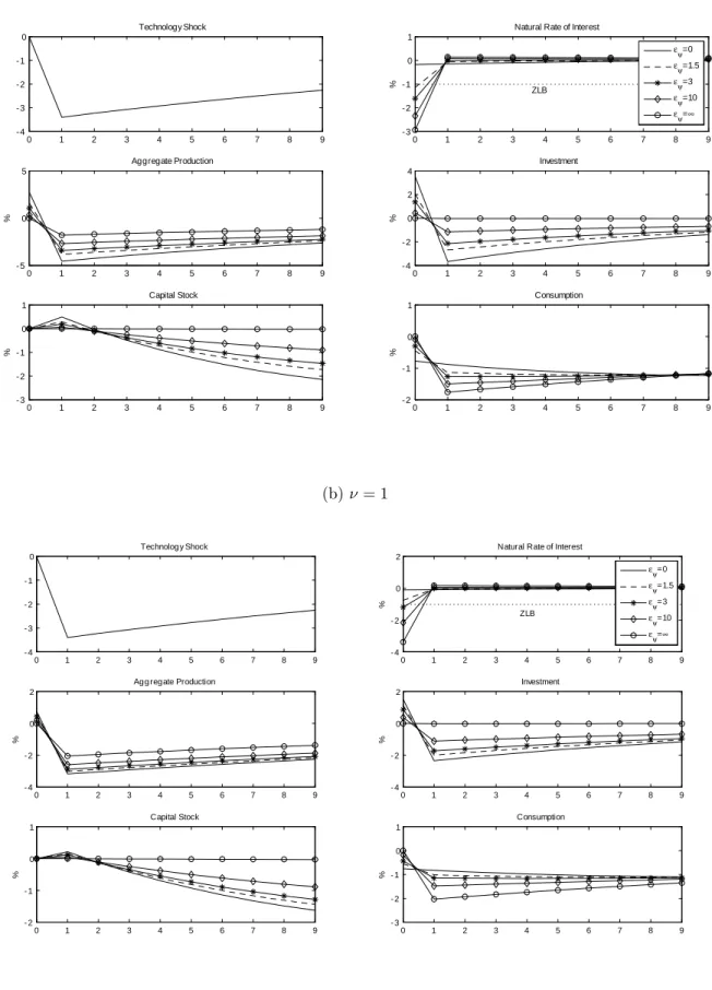
The preceding result shows that an unexpected technology shock that follows a mean reverting process such as AR(1) may not be a good candidate for explaining the underlying forces of a liquidity trap. However, equation (18) implies that, instead, a more likely candidate to account for the natural rate of interest falling below zero is a news shock that signals a decline in the expected technology level relative to the current one. Consider a perfect foresight equilibrium in which agents receive news in the initial period that a negative technology shock will hit the economy in the following period. After the shock materializes, the technology level will decay geometrically with a persistence of 0:95. In the initial period, the anticipated shock creates a sharp fall in the expected growth in technology as well as consumption. Figure 2(a) shows that the natural rate of interest will be negative for a three- standard-deviation drop in expected technology growth unless investment is extremely elastic.11 Note, however, that the declines become smaller as the adjustment cost of capital decreases. This implies that the negative impact that a liquidity trap might have on the economy is mitigated in the variable-capital model by the consumption smoothing of households.
To check the robustness of the results, we conduct a sensitivity analysis by varying the degree of relative risk aversion, c, and the inverse of the Frisch wage elasticity of labor supply, . Christiano (2004) points out that when = 1 rather than 0:11 as assumed by Woodford (2003), the ZLB will not bind for the preference shocks that
7Here, shocks other than aggregate technology shocks are suppressed for convenience.
8When capital is adjustable, the increase in current technology raises capital, and this will increase EtC^t+1j0f through c;k k;aatin equation(18). Figure 1 indicates that this e¤ect dominates the negative technology growth e¤ect when " becomes smaller and leads to an increasing consumption pro…le in some periods.
9In the log-linearized model, the natural rate of interest is less than zero when ^rtnis 100 ( 1) = = 1:01% away from its steady state level.
1 0In Woodford (2003), " = 3 is treated as a realistic value.
1 1In fact, under the baseline parameter values when " = 3, a two-standard-deviation shock is su¢cient to obtain a negative natural rate of interest.
he assumes in his variable-capital model. The logic is that the volatility of production becomes smaller when it is more costly to vary labor supply over time, which also makes the variation in consumption smaller. While this mechanism reduces the magnitude of the decline in the natural rate of interest, it still falls below zero for a three- standard-deviation technology news shock when " = 3 (Figure 2(b)). Regarding the relative risk aversion, the baseline parameter value implies a logarithmic utility function. If we assume a greater value for cthan used in the baseline case, for example one between 1 and 2, which is standard in the literature, this would make consumption less volatile while requiring a greater real interest rate response, holding the consumption pro…le …xed. Although we do not present the results here, we found that c has no signi…cant impact on whether the natural rate of interest falls below zero.
3.2 A government spending shock
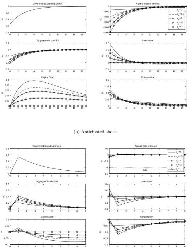
We also examine the response of the natural rate of interest to government spending shocks. To characterize the ex- ogenous process of government spending, we estimate an AR(1) model, Gt Gt =Yt= g Gt 1 Gt 1 =Yt 1+ eg;t, for the period 1970Q1-2009Q2, where Gtis real government consumption expenditure plus real gross govern- ment investment, Yt is real GDP, and variables with bars are HP-…ltered trends with a smoothing parameter of 1; 600.12 We arrive at an estimate for gof 0:75 and for the standard error of eg;t of 0:0018. Analogous to equation (18), the natural rate of interest can be expressed as ^rtj0f = 1 c;gEt gt+1+ c;k k;ggt+ c;k( k;k 1) ^Ktj0f , where c;g<0 and k;g>0. This implies that positive expected growth or an unexpected decline in government spending is required to induce a negative natural rate of interest.
In contrast to technology shocks, government spending shocks cannot cause the natural rate of interest to fall into negative territory. This is shown in Figure 3, in which the magnitude of the expected and the unexpected shock is again set to three standard deviations. Moreover, even if the size of the shocks is substantially larger, the natural rate of interest remains in positive territory. For example, it is still positive for an anticipated shock of twenty standard deviations in period 1 when " = 3.13
3.3 Preference shocks
The variable-capital model in our paper accommodates two types of preference shocks. The …rst, denoted by t, a¤ects the marginal utility of consumption, while the second, denoted by t, a¤ects the marginal disutility of labor. Although it may be di¢cult to calibrate the exogenous processes for these preference shocks, it is possible to infer which type of preference shock is more likely to cause a liquidity trap for a given level of shock. Recall that in the
1 2Data are taken from the Bureau of Economic Analysis.
1 3A shock of twenty standard deviations corresponds to an increase of approximately 3:6% in ^Gt= G=Y Gt G =G. Since in the United States G=Y ' 0:19, this means that government spending must increase by 19% from its steady state.
log-linearized model, gt is a linear combination of a government spending shock and the …rst type of preference shock, while !qt is a linear combination of a technology shock and the second type of preference shock. The preceding analysis thus indicates that whereas a preference shock that a¤ects the marginal disutility of labor may lead to a large fall in the natural rate of interest, a shock that a¤ects the marginal utility of consumption can only generate a small decline. In this context, it is interesting to note that Christiano (2004), analyzing a preference shock that is isomorphic to the …rst type of preference shock, concludes that the ZLB is unlikely to bind even when there is an extremely large shock. Our result is consistent with Christiano’s (2004) and provides an additional insight into what factors can potentially cause a liquidity trap.
The analysis in this section implies that the ZLB may bind in a variable-capital economy if a negative technology shock is anticipated and its size is su¢ciently large. Of course, in the case of the recent recession, in the wake of which short-term nominal interest rates are now close to zero not only in Japan but also in the United States and Europe, factors not taken into account in our model, such as the …nancial crisis, play a role. However, we believe that extreme pessimism with regard to the outlook for economic fundamentals may have been a factor contributing to the crisis and may have made it more di¢cult to deal with the liquidity trap in which these economies found themselves. The above results suggest that it is necessary to examine what an optimal monetary policy to respond to a negative natural rate of interest brought about by an anticipated technology shock looks like.
4 Optimal monetary policy at the ZLB
In this section, we analyze the optimal monetary policy for a central bank which has the technology to commit in a timelessly-optimal fashion (Woodford (2003)) and for a discretionary central bank that reoptimizes its behavior every period. We begin by characterizing the optimal commitment policy using a variable-capital version of the targeting rule that retains history dependence, as in the …xed-capital model. We then compare the optimal discre- tionary policy with the commitment policy as well as the discretionary policy in the …xed-capital model, with a particular focus on preemptive actions.
4.1 The optimal commitment policy
The commitment policy can be obtained by solving the Ramsey problem, which requires the minimization of the loss function, equation (17), subject to equations (10), (11), (12), (13), (14), (15), and the ZLB on the nominal interest rate, ^Rt 1 1 .14 We assume that the commitment policy is timelessly optimal, so that it can be characterized as if it has been in place from the in…nite past. After substituting out ^It, ^St, and ^t from the loss
1 4The last condition, ^Rt 1 1 , is required for the nominal interest rate to be non-negative, since the net nominal interest rate is 1 1 in the zero-in‡ation steady state.
function and the structural equations, we take the …rst-order conditions with respect to ^Yt, ^tand ^Kt+1:
0 = 1+ ! ^Yt 1gt+ !qt (! ) ^Kt 1k K^t+1 (1 ) ^Kt
+ 1t 1 1;t 1 !+ 1 2t+ 3t+ 1( y(1 (1 )) (1 )) 3;t 1; (19)
0 = 1 ^t 1 1;t 1+ 2t 2;t 1; (20)
0 = 1k2 K^t+1 (1 ) ^Kt 1k2(1 ) EtK^t+2 (1 ) ^Kt+1 + k K^t+1 K^t
k EtK^t+2 K^t+1 + kk(1 (1 )) ^Kt+1 1k ^Yt+ 1k(1 ) EtY^t+1 (! ) EtY^t+1
k(1 ) 1Etgt+1+ !Etqt+1 + 1kgt+ k!Etqt+1+ 1k 1;t 1 k(2 ) 1t+ k (1 ) Et 1;t+1
+ 1k 2t 1k(1 ) !+ Et 2;t+1+ [k (1 ) + ] 3;t 1
h
k+ (1 + ) + k (1 )2+ kf1 (1 )gi 3t+ [k (1 ) + ] Et 3;t+1; (21)
0 = 1t R^t+1 ; (22)
where 1t, 2t and 3t are the Lagrange multipliers associated with equations (10), (13) and (12), respectively. The Kuhn-Tucker condition requires that 1t >0 if and only if ^Rt = 1 1 . We show in Section B of the Appendix that 2t and 3t can be substituted out to express the …rst-order conditions in a single equation:
(1 1L)(1 3L) 1t = Et
1 L 1
1 2L 1
h^t+ 1 Y^t Y^f
tj0
i
; (23)
where denotes the …rst di¤erence and , 1 >1, 2 <1, 3 <1, and <1 are non-negative coe¢cients that depend on the structural parameters. Equation (23) expresses the condition that the central bank is required to meet by appropriately controlling the nominal interest rate. This condition nests the policy criterion for the
…xed-capital model, (1 1L)(1 3L) 1t= 0
h^t+ 1 Y^t Y^f
tj0
i
, since it is possible to check numerically that 2 = when " ! 1. Notice that equation (23) exhibits several similarities to the …xed-capital model of Jung et al. (2005) and Eggertsson and Woodford (2003a, b). First, policy responds to a linear combination of current in‡ation and the …rst di¤erence of the output gap, which is de…ned as the deviation of actual aggregate output from its natural rate, where the natural rate is de…ned following Neiss and Nelson (2003).15 Second, the lags of 1t represent policy inertia in the optimal commitment policy. If we interpret ^t+ 1 Y^t Y^tj0f as augmented in‡ation, denoted by ~t, the optimal commitment policy can be implemented through a history- dependent “in‡ation targeting scheme,” as explained below. A notable di¤erence from …xed-capital models is that the optimal commitment policy responds to a linear combination of expected future augmented in‡ation,
1 5As we argued in Section 2:3, a central bank with commitment technology maintains the consistency of its stabilization target, which is expressed in terms of natural rates as de…ned by Neiss and Nelson (2003).
which is de…ned as F~;t Et 1 1L 1 = 1 2L 1 ~t=P1j=0 jEt~t+j, where 0 = 1; 1 = 2 1; and
j= 2 j 1for j 2. The forecasts of endogenous variables matter for policy implementation due to the presence of a channel to a¤ect future states via the capital stock.
To understand the nature of the optimal commitment policy, it is useful to express equation (23) as a history- dependent in‡ation targeting rule.16 Intuitively, if the ZLB binds ( 1t >0) in period t, the subsequent policy stance will be in‡ationary. In order to implement such a policy, the central bank has a predetermined target for F~;t, denoted by F~;tT AR, and attempts to set F~;t= F~;tT ARwhenever possible. The only situation in which F~;tT ARcannot be achieved is when the ZLB prevents the central bank from providing su¢cient stimulus. In this case, the central bank simply sets the overnight interest rate to zero, which gives rise to a target shortfall of t FtT AR F~;t>0. To determine F~;tT AR, we posit that 1t = t; that is, the target shortfall is proportionate to the Lagrange multiplier on equation (10). Substituting this relationship into equation (23), we obtain the following updating rule for the target:
F~;t+1T AR = ( 1+ 3) t 1 3 t 1: (24)
Under the assumption that 1 = 2 = 0 (the ZLB has never been binding before period 0), equation (24) constitutes the in‡ation targeting rule to implement the optimal commitment policy. Clearly, the targeting rule can be interpreted as “history-dependent in‡ation-forecast targeting.” For example, suppose that t 1= 0. If the central bank fails to achieve the target due to the zero bound constraint in period t, t takes a positive value, and consequently the predetermined in‡ation target for the next period becomes higher than zero. Given the higher target, the central bank must adopt a looser policy stance, including a zero interest rate policy to raise in‡ation expectations. In sum, the optimal commitment policy in the variable-capital model …ts into the history-dependent framework, whose properties are analyzed in the …xed-capital models of Eggertsson and Woodford (2003a, b) and Iwamura et al. (2006).
On the other hand, the distinction from the …xed-capital model is that the scheme involves the central bank’s forecasts of future augmented in‡ation. When capital is adjustable, the central bank needs to take into account future developments in augmented in‡ation that are caused by expected changes in the capital stock. That is, the in‡ation-forecast targeting in the variable-capital model contains a new channel for preemptive action against future in‡ation or de‡ation. Note that there is a subtle di¤erence between preemptive action through this capital channel and the pre-shock behavior of a central bank discussed by Adam and Billi (2006, 2007) and Nakov (2005) among others in …xed-capital models. The preemptive action these papers focused on responds only to a decline in current augmented in‡ation and, more importantly, such action has no impact on future economic performance. Having said this, reactions through the existing channel of preemptive action and policy inertia are likely to be
1 6See Eggertsson and Woodford (2003a, b) and Iwamura et al. (2006) for a detailed discussion.
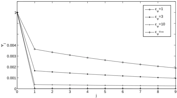
more important than those through the capital channel. To see why this might be the case, we compute the relative weights on expected augmented in‡ation, j (j = 1; 2; : : : ), for di¤erent values of " . Figure 4 shows that when = 3, the relative weights on the one-period and two-period ahead forecasts are merely 0:0019 and 0:0017, respectively. The …gure also indicates that the weights are extremely small even for a very small value of . Hence, the nature of the optimal commitment policy is largely explained by the properties already known from the
…xed-capital model.
4.2 The optimal discretionary policy
Unlike a central bank pursuing a commitment policy, one pursing a discretionary policy reoptimizes its policy every period, taking as given economic agents’ optimal behavior through which they form their expectations. Under a discretionary policy, economic agents will correctly anticipate that the central bank will set the nominal interest rate equal to the real interest rate as soon as the peril of a liquidity trap is gone. Since a promise to keep in‡ation high in the future is not credible, outcomes under a discretionary policy are suboptimal. As noted by Adam and Billi (2007), however, the inability to exploit inertial policy leads a discretionary central bank to act more preemptively than a central bank with commitment technology. Below, we focus on this aspect of discretionary policy in the variable-capital model.
The optimal discretionary policy is a time-consistent monetary policy that can be obtained by solving the following Bellman equation,
Vt K^t; st = max fY^t; ^t, ^Kt+1g
n Lt+ Vt+1 K^t+1; st+1
o
subject to equations (10), (11), (12), (13), (14), (15), and ^Rt 1 1 , given ^Kt and a vector of exogenous state variables, st. Here, the value function has a subscript t because we will assume a particular deterministic path of exogenous shocks in the numerical analysis in Section 5. In this problem, stand ^Ktare su¢cient to characterize the solution. Although a closed-form targeting rule for the optimal discretionary policy is not obtainable in the variable-capital model, the existence of this endogenous state variable distinguishes the optimal discretionary policy in the variable-capital model from that of the …xed-capital model. That is, the optimal policy decision must take into account the marginal e¤ect of variations in the capital stock on the behavior of economic agents.
More speci…cally, the capital stock can in‡uence the central bank’s decision-making in two ways. First, periodical reoptimization involves the revision of the target paths of endogenous variables (natural rates) when the central bank is unable in the previous period to match the actual level of capital to its natural rate.17 This implies that
1 7Note that a central bank with commitment technology keeps its promise to maintain the target paths of endogenous variables even if the actual capital stock deviated from the natural rate of capital as de…ned by Neiss and Nelson (2003).
a discretionary central bank wants to avoid large future deviations of capital from its own target path of capital. Therefore, if the future capital stock is expected to fall below the current target, the central bank has an incentive to encourage an increase in investment in advance to reduce the future decline in the capital stock.
In this context, an interesting question surrounding the optimal discretionary policy is whether the central bank has an incentive to raise the nominal interest rate to preemptively achieve a decumulation of capital stock to raise the natural rate of interest in the future. Such a policy may be considered as a preventive measure against falling into a liquidity trap. However, capital decumulation will make the future deviation of capital from the current target even larger when capital is already expected to decline below the natural rate in the future. For this reason, preemptively raising the nominal interest rate is costly in terms of stabilization.
The second way in which the capital stock can in‡uence the central bank’s decision-making is that a preemptive easing can strengthen the productive capacity of the actual economy through an increase of capital. More capital increases the marginal product of labor and helps reduce ine¢cient variation in consumption and labor supply when a worsening economic outlook generates signi…cant de‡ationary pressure in periods to come. As is discussed by Adam and Billi (2007), contemporaneous de‡ationary pressure that stems from the forward-looking behavior of economic agents is another reason why the central bank may choose to adopt a preemptive easing. If the central bank instead tightens its policy stance preemptively in an e¤ort to raise the future natural rate of interest, it will exacerbate the downward pressure on current in‡ation.
In sum, preemptive easing is an important policy tool for a discretionary central bank to cope with a liquidity trap caused by an anticipated technology shock. To what extent preemptive easing is important for discretionary monetary policy in the variable-capital model compared to …xed-capital models is a quantitative issue which will be addressed in the next section. Similarly, to what extent the implementation of the optimal discretionary policy entails forecasting because of the presence of capital and the lack of commitment technology is also an interesting question which will be considered below.
5 Numerical analysis
In this section, we solve the model numerically and discuss how equilibrium outcomes may di¤er under the optimal commitment and the optimal discretionary policy. In addition, we examine the nature of preemptive action taken by the discretionary central bank. For simplicity, we solve for a perfect foresight equilibrium in each exercise. In light of the results in Section 3, we assume that a technology shock will lead the ZLB to bind under the parameter values given in Table 1. The value of " is 3 unless otherwise stated. In each exercise, the economy has been in a steady state, and, in period 0, the central bank as well as economic agents receive information that the technology level will drop in the future. The size of the shock is set to 3 standard deviations, as in Section 3. If the shock
materializes in period 1, there will be an unexpected fall in the natural rate of interest in period 0. If the shock materializes later than period 1, there will be an anticipated fall in the natural rate of interest, which the optimal monetary policy will seek to counteract preemptively. In both cases, we assume that the technology shock will last for 3 periods and technology then returns to its steady-state level.
5.1 The optimal commitment and the optimal discretionary policy
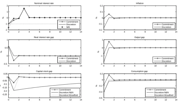
Consider an unexpected fall in the natural rate of interest in period 0, which is caused by the news that the technology level is expected to fall in period 1. Figure 5(a) shows the equilibrium paths under both types of policies. Here, real variables are expressed as the di¤erence between the actual outcome and the natural rate level. For output and the real interest rate, it turns out that the natural rate levels based on the two di¤erent de…nitions are graphically indistinguishable. Therefore, the …gure does not show separate lines for the two di¤erent de…nitions for these variables. On the other hand, the natural rate levels of capital and consumption based on Woodford’s (2003) de…nition and based on Neiss and Nelson’s (2003) de…nition clearly di¤er; hence, they are shown separately in the …gure. The reason why the natural rate of output is insensitive to which de…nition is used is that the percentage deviation of capital from its steady state level is small relative to that of labor supply. However, since the level of capital stock is large, a small variation in capital could lead to a large movement in investment. This is why the two de…nitions of natural rates lead to a large di¤erence in the natural rate of investment. Through the national income identity, equation (9), this translates into a di¤erence between the natural rate of consumption based on Neiss and Nelson (2003) and that based on Woodford (2003).
To see how the revision of target paths a¤ects equilibrium outcomes, we compare the responses under the optimal commitment policy and those under the optimal discretionary policy. In both types of policy, the nominal interest rate is lowered to the ZLB in response to a sharp decline in the natural rate of interest below zero in period 0. The inability to close the real interest rate gap in period 0 causes a recession, the depth of which depends on the policy reaction after period 1. In each period, the discretionary policy closes the real interest rate gap relative to the natural rate as de…ned by Woodford (2003) to achieve perfect stabilization in the sense that similarly-de…ned gaps for all variables are zero. However, there are persistent negative gaps for capital and consumption from their natural rates as de…ned by Neiss and Nelson (2003) since the discretionary central bank loses the incentive to aid economic recovery to the initially e¢cient paths. On the other hand, the commitment policy pushes the economy back to the targets that it has initially promised to achieve by stimulating investment in period 1, so that the level of capital stock will be closer to the natural rate of capital as de…ned by Neiss and Nelson (2003). As in the
…xed-capital model, the history-dependent nature of this policy smoothes the ‡uctuation of variables around the natural rates as de…ned by Neiss and Nelson (2003). This di¤erence in the target paths of real variables is unique
to the variable-capital model.
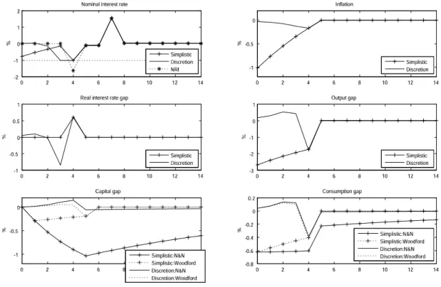
Next, let us consider an expected fall in the natural rate of interest in period 4, which follows an anticipated negative three-standard-deviation technology shock in periods 5 through 7. Since the shock is anticipated, the optimal policy can react preemptively to counter the future contraction in the production possibility frontier. From Figure 5(b), it can be seen that preemptive action under the commitment policy is fairly modest. The central bank lowers the nominal interest rate slightly below the natural rate of interest in period 3, just one period before the ZLB constraint binds. As in the …xed-capital model examined by Adam and Billi (2006), aggressive preemptive policies are relatively unimportant for a central bank with commitment technology, because policy inertia can e¤ectively stabilize the expectations of economic agents. In contrast, for a discretionary central bank, the inability to keep promises makes it necessary to react more aggressively prior to period 4. In our example, monetary easing begins in period 1 and the nominal interest rate is decreased to the ZLB from period 3 to 4. This is consistent with the …nding of Adam and Billi (2007), although the motive for preemptive action is slightly more complicated in the variable-capital model than in the …xed-capital model.
As in …xed-capital models, the de‡ationary pressure stemming from the forward-looking behavior of economic agents who rationally anticipate the future shock needs to be mitigated. In addition, the discretionary central bank recognizes that future central bank decisions will not necessarily be consistent with current decisions. Naturally, the discretionary central bank has an incentive to prevent future natural rates to deviate greatly from the paths that it perceives to be desirable. Speci…cally, before the shock, the central bank engages in monetary easing in successive steps to stimulate consumption, investment and aggregate output to levels that exceed their natural levels. These e¤orts not only counteract part of the de‡ationary pressure arising from period 4, but also push up the capital stock to exceed the natural rate level. In period 5, capital begins to fall due to the positive real interest rate gap in period 4. However, in period 5, the negative capital gap relative to the natural rate as de…ned by Neis and Nelson (2003) is much smaller than that in period 1 in Figure 5(a), since capital was already accumulated in earlier periods well above the natural rate as de…ned by Neiss and Nelson (2003). In fact, the level of capital is close to the commitment outcome. As the level of capital in period 5 is close to the natural rate as de…ned by Neiss and Nelson (2003) when the preemptive policy has been implemented, it is not surprising that, after period 5, the policy outcome is closer to the commitment case in Figure 5(b) than in Figure 5(a). Clearly, the capital and consumption gaps relative to their natural rates as de…ned by Neiss and Nelson (2003) in Figure 5(b) are considerably smaller than in Figure 5(a), where the central bank had no time to encourage the build-up of a bu¤er stock of capital. These results indicate that although the outcome of the optimal discretionary policy is inferior to the commitment outcome, particularly before period 5, such a policy can nevertheless improve welfare in the sense that gaps relative to the natural rates as de…ned by Neiss and Nelson (2003) become smaller if the central bank has time to act preemptively.
To highlight this point further, we consider a simplistic rule of the form ^Rt = maxnr^tn+ Et^t+1;1 1= o. This policy controls the nominal interest rate in such a way that the real interest rate is equal to the natural rate of interest as de…ned by Woodford (2003) whenever possible, which is su¢cient to achieve perfect stabilization after a negative natural-rate-of-interest shock. As Figure 6 shows, however, under such a simplistic rule, the nominal interest rate is raised in periods 2 and 3 to close the real interest rate gap. As a result, not only is the recession exacerbated, but the negative capital gap relative to its natural rate as de…ned by Neiss and Nelson (2003) also becomes enormous. Even though all gaps from the natural rates as de…ned by Woodford (2003) will be zero in and after period 5 under the simplistic policy, the capital and consumption gaps relative to their natural rates as de…ned by Neiss and Nelson (2003) are unambiguously larger than under the optimal discretionary policy. This example illustrates that an inappropriate policy response in anticipation of a liquidity trap may be detrimental to the economy even after the danger has passed. Such a policy implication for a central bank without commitment technology does not exist in …xed-capital models or even in models with in‡ation inertia (but without capital) where future natural rates are independent of the history of economic outcomes.18
5.2 Preemptive policy and the variability of capital
How does the variability of capital a¤ect equilibrium outcomes before and during the liquidity trap? To address this question, we compare the equilibrium outcomes under the optimal discretionary policy when " = 3 and 500. In Figure 7, equilibrium outcomes are expressed in gaps relative to the natural rates as de…ned by Neiss and Nelson (2003). The …gure shows that the in‡ation and consumption gaps are smaller and smoother as capital becomes more variable. That is, given the magnitude of the technology shock, the di¤erences in the in‡ation and consumption paths under commitment and discretion are smaller the more variable capital becomes. The reason why the suboptimality of discretion shrinks is that, …rst, more variable capital leads to a smaller fall in the natural rate of interest in period 4, as we saw in Section 3. When the same technology shock translates into a smaller natural-rate-of-interest shock, the impact on in‡ation and the output gap will be smaller. And second, an increase in capital caused by preemptive easing contributes to increases in the production capacity in post-liquidity-trap periods, thereby mitigating at least partially the decline in in‡ation and output in pre-liquidity-trap periods. As a result, the optimal discretionary policy does not need to cut the nominal interest rate as far in advance as in the
…xed-capital environment, as Figure 7 indicates.
1 8In models with in‡ation inertia, natural rates do not depend on lagged in‡ation since in‡ation is constant in a ‡exible-price economy.
5.3 Is forecasting important for the optimal discretionary policy?
The optimal discretionary policy has no closed-form representation and it is not clear which variables play a critical role for the implementation of the policy. Moreover, the exposition in Section 4:2 does not answer to what extent the presence of capital and the ZLB makes the forecasting of future economic variables important when a discretionary central bank takes preemptive action. In order to address these issues, we consider a policy which attempts to satisfy the following relationship whenever possible:
0 =h^t+ 1 Y^t Y^tn i: (25)
When the ZLB prevents the policy from meeting this criterion, the nominal interest rate is set to zero and the right hand side of equation (25), which can be viewed as augmented in‡ation for the discretionary policy, is negative. The implementation criterion of the optimal discretionary policy in the …xed-capital model has the same representation as equation (25) and this static policy is su¢cient to achieve perfect stabilization in the variable-capital model if the ZLB does not bind in any period. This means that the comparison of equilibrium outcomes under the optimal discretionary policy and the …xed-capital policy, equation (25), can provide us with some information on whether forecasting is critical in determining to what extent preemptive action taken by a discretionary central bank will be successful.
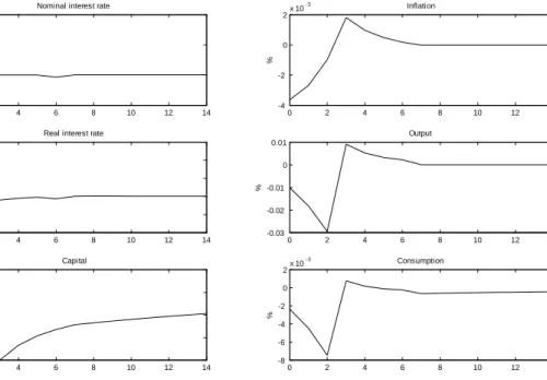
Figure 8 presents the di¤erences in equilibrium outcomes when monetary policy follows the optimal discretionary rule and the …xed-capital rule. In each panel, the equilibrium outcome under the …xed-capital rule is subtracted from that of the optimal discretionary policy. Clearly, the magnitudes of the di¤erences in each panel are extremely small. For example, the nominal interest rate di¤ers by no more than 1 basis point except in period 2, where the di¤erence is still only 1:6 basis points. Consequently, the impact of forecasting on outcomes in the optimal discretionary policy is quantitatively small in our model. The gains from forecasting future variables are limited since the current variables re‡ect a su¢cient amount of information about the future recession through the forward- looking behavior of private agents. Moreover, our result suggests that, despite the introduction of investment in the model, the optimal discretionary policy can be approximated well with a criterion which only includes a linear combination of in‡ation and the output gap. Note that the output gap is measured by the distance from the natural rate of output following Woodford’s de…nition (2003) rather than from that when capital is …xed. This carries the practical implication that a discretionary central bank should make greater e¤orts to precisely measure current in‡ation and the natural rate of output than to accurately forecast their future values.