Sparse Additive Matrix Factorization for Robust PCA
and Its Generalization
Shinichi Nakajima [email protected]
Nikon Corporation, Tokyo, 140-8601, Japan
Masashi Sugiyama [email protected]
Tokyo Institute of Technology, Tokyo 152-8552, Japan
S. Derin Babacan [email protected]
Beckman Institute, University of Illinois at Urbana-Champaign, Urbana, IL 61801, USA
Editor:Steven C.H. Hoi and Wray Buntine
Abstract
Principal component analysis (PCA) can be regarded as approximating a data matrix with a low-rank one by imposing sparsity on its singular values, and its robust variant further captures sparse noise. In this paper, we extend such sparse matrix learning methods, and propose a novel unified framework called sparse additive matrix factorization (SAMF). SAMF systematically induces various types of sparsity by the so-called model-induced reg- ularizationin the Bayesian framework. We propose an iterative algorithm called the mean update (MU) for the variational Bayesian approximation to SAMF, which gives the global optimal solution for a large subset of parameters in each step. We demonstrate the useful- ness of our method on artificial data and the foreground/background video separation. Keywords: Variational Bayes, Robust PCA, Matrix Factorization, Sparsity, Model- induced Regulariztion
1. Introduction
Principal component analysis (PCA) (Hotelling, 1933) is a classical method for obtaining low-dimensional expression of data. PCA can be regarded as approximating a data ma- trix with a low-rank one by imposing sparsity on its singular values. A robust variant of PCA further copes with sparse spiky noise included in observations (Candes et al., 2009; Babacan et al.,2012).
In this paper, we extend the idea of robust PCA, and propose a more general framework called sparse additive matrix factorization (SAMF). The proposed SAMF can handle various types of sparse noise such as row-wise and column-wise sparsity, in addition to element-wise sparsity (spiky noise) and low-rank sparsity (low-dimensional expression); furthermore, their arbitrary additive combination is also allowed. In the context of robust PCA, row-wise and column-wise sparsity can capture noise observed when some sensors are broken and their outputs are always unreliable, or some accident disturbs all sensor outputs at a time.
Technically, our approach induces sparsity by the so-called model-induced regularization (MIR) (Nakajima and Sugiyama,2011). MIR is an implicit regularization property of the Bayesian approach, which is based on one-to-many (i.e., redundant) mapping of parameters and outcomes (Watanabe,2009). In the case of matrix factorization, an observed matrix is
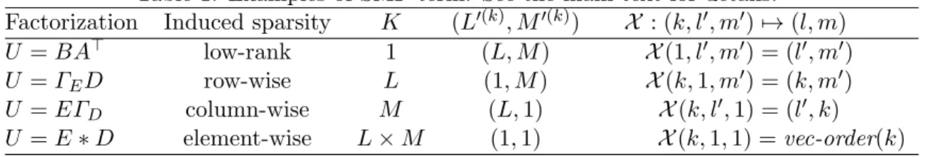
Table 1: Examples of SMF term. See the main text for details. Factorization Induced sparsity K (L′(k), M′(k)) X : (k, l′, m′) 7→ (l, m) U = BA⊤ low-rank 1 (L, M ) X (1, l′, m′) = (l′, m′) U = ΓED row-wise L (1, M ) X (k, 1, m′) = (k, m′) U = EΓD column-wise M (L, 1) X (k, l′, 1) = (l′, k) U = E ∗ D element-wise L × M (1, 1) X (k, 1, 1) = vec-order(k)
decomposed into two redundant matrices, which was shown to induce sparsity in the singular values under the variational Bayesian approximation (Nakajima and Sugiyama,2011).
We also show that MIR in SAMF can be interpreted as automatic relevance determi- nation (ARD) (Neal, 1996), which is a popular Bayesian approach to inducing sparsity. Nevertheless, we argue that the MIR formulation is more preferable since it allows us to derive a practically useful algorithm called the mean update (MU) from a recent theoreti- cal result (Nakajima et al.,2011): the MU algorithm is based on the variational Bayesian approximation, and gives the global optimal solution for a large subset of parameters in each step. Through experiments, we show that the MU algorithm compares favorably with a standard iterative algorithm for variational Bayesian inference. We also demonstrate the usefulness of SAMF in foreground/background video separation, where sparsity is induced based on image segmentation.
2. Formulation
In this section, we formulate the sparse additive matrix factorization (SAMF) model. 2.1. Examples of Factorization
In ordinary MF, an observed matrix V ∈ RL×M is modeled by a low rank target matrix U ∈ RL×M contaminated with a random noise matrix E ∈ RL×M.
V = U + E.
Then the target matrix U is decomposed into the product of two matrices A ∈ RM ×H and B ∈ RL×H:
Ulow-rank= BA⊤=
∑H h=1
bha⊤h, (1)
where ⊤ denotes the transpose of a matrix or vector. Throughout the paper, we denote a column vector of a matrix by a bold smaller letter, and a row vector by a bold smaller letter with a tilde:
A = (a1, . . . , aH) = (ea1, . . . ,eaM)⊤, B = (b1, . . . , bH) = (eb1, . . . , ebL)⊤.
�→
G
U =
U1,1 U1,2 U1,3 U1,4 U2,1 U2,2 U2,3 U2,4 U3,1 U3,2 U3,3 U3,4 U4,1 U4,2 U4,3 U4,4
U�(1)
=�U1,1 U1,2 U1,3 U1,4
�
= B(1)A(1)� U�(2)
=
�U2,1 U2,2 U2,3 U2,4
�
= B(2)A(2)� U�(3)=�U3,1 U3,2 U4,1 U4,4�= B(3)A(3)� U�(4)
=�U3,3 U4,3
�
= B(4)A(4)� U�(5)
=�U3,4
�
= B(5)A(5)� U�(6)
=�U4,2
�
= B(6)A(6)�
�→
� G �
�
�→
� G
�→
� G
�
�
�
�
�
�
Figure 1: An example of SMF term construc- tion. G(·; X ) with X : (k, l′, m′) 7→ (l, m) maps the set {U′(k)}Kk=1 of the PR matrices to the target ma- trix U , so that Ul′(k)′,m′ = UX(k,l′,m′)= Ul,m.
�→
G
U =�UU1,1 U1,2 U1,3 2,1 U2,2 U2,3
� U�(1)
=�U1,1 U1,2 U1,3�= B(1)A(1)� U�(2)
=�U2,1 U2,2 U2,3�= B(2)A(2)�
�→
G
U =�UU1,1 U1,2 U1,3 2,1 U2,2 U2,3
� U
�(1)=�U1,1
U2,1
�
= B(1)A(1)�
U�(2)
=
�U1,2 U2,2
�
= B(2)A(2)� U�(3)=�U1,3
U2,3
�
= B(3)A(3)�
�→
G
U =�UU1,1 U1,2 U1,3 2,1 U2,2 U2,3
� U�(1)
=�U1,1
�
= B(1)A(1)�
U�(6)=�U2,3�= B(6)A(6)� U�(2)=�U2,1�= B(2)A(2)�
U�(3)=�U1,2�= B(3)A(3)�
U�(4)=�U2,2�= B(4)A(4)� U�(5)
=�U1,3
�
= B(5)A(5)�
Figure 2: SMF construction for the row- wise (top), the column-wise (middle), and the element-wise (bottom) sparse terms.
The last equation in Eq.(1) implies that the plain matrix product (i.e., BA⊤) is the sum of rank-1 components. It was elucidated that this product induces an implicit reg- ularization effect called model-induced regularization (MIR), and a low-rank (singular- component-wise sparse) solution is produced under the variational Bayesian approximation (Nakajima and Sugiyama,2011).
Let us consider other types of factorization:
Urow= ΓED = (γ1ede1, . . . , γLeedL)⊤, (2) Ucolumn = EΓD = (γd1e1, . . . , γMd eM), (3) where ΓD = diag(γ1d, . . . , γMd ) ∈ RM ×M and ΓE = diag(γ1e, . . . , γLe) ∈ RL×L are diagonal matrices, and D, E ∈ RL×M. These examples are also matrix products, but one of the factors is restricted to be diagonal. Because of this diagonal constraint, the l-th diagonal entry γle in ΓE is shared by all the entries in the l-th row of Urow as a common factor. Similarly, the m-th diagonal entry γmd in ΓD is shared by all the entries in the m-th column of Ucolumn.
Another example is the Hadamard (or element-wise) product:
Uelement= E ∗ D, where (E ∗ D)l,m= El,mDl,m. (4) In this factorization form, no entry in E and D is shared by more than one entry in Uelement. In fact, the forms (2)–(4) of factorization induce different types of sparsity, through the MIR mechanism. In Section2.2, they will be derived as a row-wise, a column-wise, and an element-wise sparsity inducing terms, respectively, within a unified framework.
2.2. A General Expression of Factorization
Our general expression consists of partitioning, rearrangement, and factorization. The following is the form of a sparse matrix factorization (SMF) term:
U = G({U′(k)}Kk=1; X ), where U′(k)= B(k)A(k)⊤. (5)
Figure 1shows how to construct an SMF term. First, we partition the entries of U into K parts. Then, by rearranging the entries in each part, we form partitioned-and-rearranged (PR) matrices U′(k)∈ RL′(k)×M′(k)for k = 1, . . . , K. Finally, each of U′(k)is decomposed into the product of A(k)∈ RM′(k)×H′(k) and B(k)∈ RL′(k)×H′(k), where H′(k)≤ min(L′(k), M′(k)). In Eq.(5), the function G(·; X ) is responsible for partitioning and rearrangement: It maps the set {U′(k)}Kk=1 of the PR matrices to the target matrix U ∈ RL×M, based on the one-to-one map X : (k, l′, m′) 7→ (l, m) from indices of the entries in {U′(k)}Kk=1 to indices of the entries in U , such that
(G({U′(k)}Kk=1; X ))
l,m= Ul,m= UX(k,l′,m′)= U
′(k)
l′,m′. (6)
As will be discussed in Section 4.1, the SMF term expression (5) under the variational Bayesian approximation induces low-rank sparsity in each partition. Therefore, partition- wise sparsity is induced, if we design a SMF term so that {U′(k)} for all k are rank-1 matrices (i.e., vectors).
Let us, for example, assume that row-wise sparsity is required. We first make the row-wise partition, i.e., separate U ∈ RL×M into L pieces of M -dimensional row vectors U′(l) = ue⊤l ∈ R1×M. Then, we factorize each partition as U′(l) = B(l)A(l)⊤ (see the top illustration in Figure2). Thus, we obtain the row-wise sparse term (2). Here, X (k, 1, m′) = (k, m′) makes the following connection between Eqs.(2) and (5): γle= B(k)∈ R, edl= A(k)∈ RM ×1 for k = l. Similarly, requiring column-wise and element-wise sparsity leads to Eqs.(3) and (4), respectively (see the bottom two illustrations in Figure 2). Table 1 summarizes how to design these SMF terms, where vec-order(k) = (1 + ((k − 1) mod L), ⌈k/L⌉) goes along the columns one after another in the same way as the vec operator forms a vector by stacking the columns of a matrix (in other words, (U′(1), . . . , U′(K))⊤= vec(U )).
In practice, SMF terms should be designed based on side information. In robust PCA (Candes et al., 2009; Babacan et al., 2012), the element-wise sparse term is added to the low-rank term for the case where the observation is expected to contain spiky noise. Here, we can say that the ‘expectation of spiky noise’ is used as side information. Using the SMF expression (5), we can similarly add a row-wise term and/or a column-wise term when the corresponding type of sparse noise is expected.
The SMF expression enables us to use side information in a more flexible way. In Section 5.2, we apply our method to a foreground/background video separation problem, where moving objects are considered to belong to the foreground. The previous approach (Candes et al.,2009;Babacan et al.,2012) adds an element-wise sparse term for capturing the moving objects. However, we can also use a natural assumption that the pixels in an image segment with similar intensity values tend to belong to the same object and hence share the same label. To use this side information, we adopt a segment-wise sparse term, where the PR matrix is constructed based on a precomputed over-segmented image. We will show in Section 5.2 that the segment-wise sparse term captures the foreground more accurately than the element-wise sparse term.
The SMF expression also provides a unified framework where a single theory can be applied to various types of factorization. Based on this framework, we derive a useful algorithm for variational approximation in Section 3.
2.3. Formulation of SAMF
We define a sparse additive matrix factorization (SAMF) model as a sum of SMF terms (5):
V =∑Ss=1U(s)+ E, (7)
where U(s)= G({B(k,s)A(k,s)⊤}Kk=1(s); X(s)). (8) Let us summarize the parameters as follows:
Θ = {Θ(s)A , Θ(s)B }Ss=1,
where Θ(s)A = {A(k,s)}Kk=1(s), ΘB(s)= {B(k,s)}Kk=1(s).
As in the probabilistic MF (Salakhutdinov and Mnih, 2008), we assume independent Gaussian noise and priors. Thus, the likelihood and the priors are written as
p(V |Θ) ∝ exp (
− 1 2σ2
V −∑Ss=1U(s)
2
Fro
)
, (9)
p({ΘA(s)}Ss=1) ∝ exp(−1 2·
∑S s=1
∑K(s) k=1 tr
(A(k,s)CA(k,s)−1A(k,s)⊤)), (10)
p({ΘB(s)}Ss=1) ∝ exp(−1 2·
∑S s=1
∑K(s) k=1 tr
(B(k,s)CB(k,s)−1B(k,s)⊤)), (11)
where ∥ · ∥Fro and tr(·) denote the Frobenius norm and the trace of a matrix, respectively. We assume that the prior covariances of A(k,s) and B(k,s) are diagonal and positive-definite:
CA(k,s)= diag(c(k,s)2a1 , . . . , c(k,s)2aH ), CB(k,s)= diag(c(k,s)2b
1 , . . . , c(k,s)2b
H ).
Without loss of generality, we assume that the diagonal entries of CA(k,s)CB(k,s) are arranged in the non-increasing order, i.e., c(k,s)ah c(k,s)b
h ≥ c
(k,s) ah′ c(k,s)b
h′ for any pair h < h′. 2.4. Variational Bayesian Approximation
The Bayes posterior is written as
p(Θ|V ) = p(V |Θ)p(Θ)
p(V ) , (12)
where p(V ) = ⟨p(V |Θ)⟩p(Θ) is the marginal likelihood. Here, ⟨·⟩p denotes the expectation over the distribution p. Since the Bayes posterior (12) is computationally intractable, the variational Bayesian (VB) approximation was proposed (Bishop,1999;Lim and Teh,2007; Ilin and Raiko, 2010;Babacan et al.,2012).
Let r(Θ), or r for short, be a trial distribution. The following functional with respect to r is called the free energy:
F (r|V ) =
⟨
log r(Θ) p(Θ|V )
⟩
r(Θ)
− log p(V ). (13)
The first term is the Kullback-Leibler (KL) distance from the trial distribution to the Bayes posterior, and the second term is a constant. Therefore, minimizing the free energy (13) amounts to finding a distribution closest to the Bayes posterior in the sense of the KL distance. In the VB approximation, the free energy (13) is minimized over some restricted function space.
Following the standard VB procedure (Bishop,1999;Lim and Teh,2007;Babacan et al., 2012), we impose the following decomposability constraint on the posterior:
r(Θ) =∏Ss=1r(s)A (ΘA(s))rB(s)(ΘB(s)). (14) Under this constraint, it is easy to show that the VB posterior minimizing the free energy (13) is written as
r(Θ) =
∏S s=1
K∏(s) k=1
(M′(k,s)
∏
m′=1
NH′(k,s)(ae(k,s)m′ ; eab(k,s)m′ , ΣA(k,s)) ·
L∏′(k,s) l′=1
NH′(k,s)(eb(k,s)l′ ; ebb(k,s)l′ , ΣB(k,s)) )
, (15) where Nd(·; µ, Σ) denotes the d-dimensional Gaussian distribution with mean µ and co- variance Σ.
3. Algorithm for SAMF
In this section, we first give a theorem that reduces a partial SAMF problem to the ordinary MF problem, which can be solved analytically. Then we derive an algorithm for the entire SAMF problem.
3.1. Key Theorem
Let us denote the mean of U(s), defined in Eq.(8), over the VB posterior by Ub(s)= ⟨U(s)⟩r(s)
A (Θ (s) A )r
(s) B (Θ
(s) B )
= G({ bB(k,s)Ab(k,s)⊤}Kk=1(s); X(s)). (16) Then we obtain the following theorem (the proof is omitted because of the space limitation): Theorem 1 Given{ bU(s′)}s′̸=sand the noise varianceσ2, the VB posterior of(Θ(s)A , ΘB(s)) = {A(k,s), B(k,s)}Kk=1(s) coincides with the VB posterior of the following MF model:
p(Z′(k,s)|A(k,s), B(k,s)) ∝ exp (
− 1 2σ2
Z′(k,s)− B(k,s)A(k,s)⊤ 2Fro )
, (17)
p(A(k,s)) ∝ exp (
−1 2tr
(
A(k,s)CA(k,s)−1A(k,s)⊤)), (18)
p(B(k,s)) ∝ exp (
−1 2tr
(B(k,s)CB(k,s)−1B(k,s)⊤)), (19)
for each k = 1, . . . , K(s). Here, Z′(k,s) ∈ RL′(k,s)×M′(k,s) is defined as Zl′(k,s)′,m′ = ZX(s)(s)(k,l′,m′), where Z(s)= V −∑
s′̸=s
Ub(s). (20)
The left formula in Eq.(20) relates the entries of Z(s) ∈ RL×M to the entries of {Z′(k,s) ∈ RL′(k,s)×M′(k,s)}k=1K(s) by using the map X(s): (k, l′, m′) 7→ (l, m) (see Eq.(6) and Figure1).
When the noise variance σ2 is unknown, the following lemma is useful (the proof is omitted):
Lemma 2 Given the VB posterior for {ΘA(s), ΘB(s)}Ss=1, the noise variance σ2 minimizing the free energy (13) is given by
σ2 = 1 LM
{∥V ∥2Fro− 2
∑S s=1
tr (
Ub(s)⊤ (
V −
∑S s′=s+1
Ub(s′) ))
+∑Ss=1∑Kk=1(s)tr(( bA(k,s)⊤Ab(k,s)+ M′(k,s)ΣA(k,s)) · ( bB(k,s)⊤Bb(k,s)+ L′(k,s)ΣB(k,s)))}. (21) 3.2. Partial Analytic Solution
Theorem 1 allows us to utilize the results given in Nakajima et al. (2011), which give the global analytic solution for VBMF. Combining Theorem 1 above and Corollaries 1–3 in Nakajima et al.(2011), we obtain the following corollaries. Below, we assume that L′(k,s)≤ M′(k,s) for all (k, s). We can always take the mapping X(s) so, without any practical restriction.
Corollary 1 Assume that { bU(s′)}s′̸=sand the noise variance σ2 are given. Letγ(k,s)h (≥ 0) be the h-th largest singular value of Z′(k,s), and let ω(k,s)ah and ω(k,s)b
h be the associated right and left singular vectors:
Z′(k,s) =
L∑′(k,s) h=1
γh(k,s)ω(k,s)b
h ω
(k,s)⊤ ah .
Let bγh(k,s) be the second largest real solution of the following quartic equation with respect to t:
fh(t) := t4+ ξ3(k,s)t3+ ξ2(k,s)t2+ ξ1(k,s)t + ξ0(k,s)= 0, (22) where the coefficients are defined by
ξ3(k,s)= (L
′(k,s)− M′(k,s))2γ(k,s) h
L′(k,s)M′(k,s) , ξ2(k,s)= −
ξ3γh(k,s)+
(L′(k,s)2+ M′(k,s)2)η(k,s)2h L′(k,s)M′(k,s) +
2σ4 c(k,s)2ah c
(k,s)2 bh
,
ξ1(k,s)= ξ3(k,s)
√ ξ(k,s)0 , ξ0(k,s)=
η(k,s)2h − σ
4
c(k,s)2ah c
(k,s)2 bh
2
,
η(k,s)2h = (
1 −σ
2L′(k,s)
γh(k,s)2 ) (
1 −σ
2M′(k,s)
γh(k,s)2 )
γh(k,s)2.
Let
eγh(k,s)=
√
τ +√τ2− L′(k,s)M′(k,s)σ4, (23)
where
τ = (L
′(k,s)+ M′(k,s))σ2
2 +
σ4 2c(k,s)2ah c
(k,s)2 bh
. Then, the global VB solution can be expressed as
Ub′(k,s)VB= ( bB(k,s)Ab(k,s)⊤)VB=
H∑′(k,s) h=1
bγh(k,s)VBω (k,s) bh ω
(k,s)⊤ ah ,
where bγh(k,s)VB=
{bγh(k,s) if γ (k,s)
h > eγh(k,s),
0 otherwise. (24)
Corollary 2 Given { bU(s′)}s′̸=s and the noise variance σ2, the global empirical VB so- lution is given by
Ub′(k,s)EVB =
H∑′(k,s) h=1
bγh(k,s)EVBω (k,s) bh ω
(k,s)⊤ ah ,
where bγh(k,s)EVB=
{˘γh(k,s)VB if γh(k,s)> γ(k,s)h and∆(k,s)h ≤ 0,
0 otherwise. (25)
Here,
γ(k,s)h = (√L′(k,s)+√M′(k,s))σ, (26)
˘
c(k,s)2h = 1 2L′(k,s)M′(k,s)
(γh(k,s)2− (L′(k,s)+ M′(k,s))σ2
+√(γ(k,s)2h − (L′(k,s)+ M′(k,s))σ2)2− 4L′(k,s)M′(k,s)σ4 )
, (27)
∆(k,s)h = M′(k,s)log
( γh(k,s) M′(k,s)σ2˘γ
(k,s)VB
h + 1
)
+ L′(k,s)log
( γh(k,s) L′(k,s)σ2γ˘
(k,s)VB
h + 1
)
+ 1 σ2
(−2γh(k,s)γ˘(k,s)VBh + L′(k,s)M′(k,s)˘c(k,s)2h ), (28)
and ˘γh(k,s)VB is the VB solution for c(k,s)ah c
(k,s) bh = ˘c
(k,s)
h .
Corollary 3 Given { bU(s′)}s′̸=s and the noise variance σ2, the VB posteriors are given by
rAVB(k,s)(A(k,s)) =
H∏′(k,s) h=1
NM′(k,s)(a(k,s)h ;ab(k,s)h , σ(k,s)2ah IM′(k,s)),
rVBB(k,s)(B(k,s)) =
H∏′(k,s) h=1
NL′(k,s)(b(k,s)h ; bb(k,s)h , σb(k,s)2
h IL′(k,s)),
where, for bγh(k,s)VB being the solution given by Corollary 1, b
a(k,s)h = ±
√
bγh(k,s)VBbδh(k,s)· ω(k,s)ah , bb
(k,s)
h = ±
√
bγh(k,s)VBδb(k,s)−1h · ω(k,s)bh ,
σa(k,s)2h = 1
2M′(k,s)(bγh(k,s)VBbδh(k,s)−1+ σ2c(k,s)−2ah )
{
−(ηb(k,s)2h − σ2(M′(k,s)− L′(k,s)))
+
√
(bηh(k,s)2− σ2(M′(k,s)− L′(k,s)))2+ 4M′(k,s)σ2ηbh(k,s)2 }
,
σb(k,s)2
h =
1
2L′(k,s)(bγh(k,s)VBδb(k,s)h + σ2c(k,s)−2b
h )
{
−(bη(k,s)2h + σ2(M′(k,s)− L′(k,s)))
+
√
(bηh(k,s)2+ σ2(M′(k,s)− L′(k,s)))2+ 4L′(k,s)σ2ηbh(k,s)2
} ,
bδh(k,s)= 1
2σ2M′(k,s)c(k,s)−2ah
{
(M′(k,s)− L′(k,s))(γh(k,s)− bγ(k,s)VBh )
+ vu
t(Mu ′(k,s)− L′(k,s))2(γh(k,s)− bγh(k,s)VB)2+4σ
4L′(k,s)M′(k,s)
c(k,s)2ah c
(k,s)2 bh
} ,
b ηh(k,s)2=
ηh(k,s)2 if γh(k,s) > eγh(k,s),
σ4
c(k,s)2ah c(k,s)2bh otherwise.
When σ2 is known, Corollary 1and Corollary 2provide the global analytic solution of the partial problem, where the variables on which { bU(s′)}s′̸=sdepends are fixed. Note that they give the global analytic solution for single-term (S = 1) SAMF.
3.3. Mean Update Algorithm
Using Corollaries 1–3 and Lemma 2, we propose an algorithm for SAMF, called the mean update (MU). We describe its pseudo-code in Algorithm1, where 0(d1,d2)denotes the d1× d2
matrix with all entries equal to zero.
Although each of the corollaries and the lemma above guarantee the global optimality for each step, the MU algorithm does not generally guarantee the simultaneous global optimality over the entire parameter space. Nevertheless, experimental results in Section5 show that the MU algorithm performs very well in practice.
4. Discussion
In this section, we first discuss the relation between MIR and ARD. Then, we introduce the standard VB iteration for SAMF, which is used as a baseline in the experiments. 4.1. Relation between MIR and ARD
The MIR effect (Nakajima and Sugiyama, 2011) induced by factorization actually has a close connection to the automatic relevance determination (ARD) effect (Neal,1996). As-
Algorithm 1 Mean update (MU) algorithm for (empirical) VB SAMF.
1: Initialization: bU(s)← 0(L,M ) for s = 1, . . . , S, σ2← ∥V ∥2Fro/(LM ).
2: fors = 1 to S do
3: The (empirical) VB solution of U′(k,s) = B(k,s)A(k,s)⊤ for each k = 1, . . . , K(s), given { bU(s′)}s′̸=s, is computed by Corollary1 (Corollary 2).
4: Ub(s)← G({ bB(k,s)Ab(k,s)⊤}K(s) k=1; X(s)). 5: end for
6: σ2 is estimated by Lemma 2, given the VB posterior on {Θ(s)A , Θ(s)B }Ss=1 (computed by Corollary3).
7: Repeat 2 to 6 until convergence.
sume that CA= IH, where Id denotes the d-dimensional identity matrix, in the plain MF model (17)–(19) (here we omit the suffixes k and s for brevity), and consider the following transformation: BA⊤7→ U ∈ RL×M. Then, the likelihood (17) and the prior (18) on A are rewritten as
p(Z′|U ) ∝ exp (
− 1 2σ2∥Z
′− U ∥2 Fro
)
, (29)
p(U |B) ∝ exp (
−1 2tr
(U⊤(BB⊤)†U)), (30)
where † denotes the Moore-Penrose generalized inverse of a matrix. The prior (19) on B is kept unchanged. p(U |B) in Eq.(30) is so-called the ARD prior with the covariance hyper- parameter BB⊤ ∈ RL×L. It is known that this induces the ARD effect, i.e., the empirical Bayesian procedure where the hyperparameter BB⊤ is also estimated from observations induces strong regularization and sparsity (Neal, 1996) (see also Efron and Morris (1973) for a simple Gaussian case).
In the current context, Eq.(30) induces low-rank sparsity on U if no restriction on BB⊤ is imposed. Similarly, we can show that (γle)2 in Eq.(2) plays a role of the prior variance shared by the entries in uel∈ RM, (γmd)2 in Eq.(3) plays a role of the prior variance shared by the entries in um∈ RL, and El,m2 in Eq.(4) plays a role of the prior variance on Ul,m∈ R, respectively. This explains the mechanism how the factorization forms in Eqs.(2)–(4) induce row-wise, column-wise, and element-wise sparsity, respectively.
When we employ the SMF term expression (5), MIR occurs in each partition. Therefore, low-rank sparsity in each partition is observed. Corollary 1 and Corollary 2 theoretically support this fact: Small singular values are discarded by thresholding in Eqs.(24) and (25). 4.2. Standard VB Iteration
Following the standard procedure for the VB approximation (Bishop, 1999; Lim and Teh, 2007;Babacan et al.,2012), we can derive the following algorithm, which we call the stan-
dard VB iteration:
Ab(k,s)= σ−2Z′(k,s)⊤Bb(k,s)ΣA(k,s), (31)
ΣA(k,s)= σ2(Bb(k,s)⊤Bb(k,s)+L′(k,s)ΣB(k,s)+σ2CA(k,s)−1)−1, (32)
Bb(k,s)= σ−2Z′(k,s)Ab(k,s)ΣB(k,s), (33)
ΣB(k,s)= σ2(Ab(k,s)⊤Ab(k,s)+M′(k,s)ΣA(k,s)+σ2CB(k,s)−1)−1. (34) Iterating Eqs.(31)–(34) for each (k, s) in turn until convergence gives a local minimum of the free energy (13).
In the empirical Bayesian scenario, the hyperparameters {CA(k,s), CB(k,s)}Kk=1,(s)Ss=1 are also estimated from observations. The following update rules give a local minimum of the free energy:
c(k,s)2ah = ∥ab(k,s)h ∥2/M′(k,s)+ (ΣA(k,s))hh, (35) c(k,s)2b
h = ∥bb
(k,s)
h ∥2/L′(k,s)+ (Σ (k,s)
B )hh. (36)
When the noise variance σ2 is unknown, it is estimated by Eq.(21) in each iteration. The standard VB iteration is computationally efficient since only a single parameter in { bA(k,s), ΣA(k,s), bB(k,s), ΣB(k,s), c(k,s)2ah , c(k,s)2b
h }
K(s)
k=1,Ss=1 is updated in each step. However, it is known that the standard VB iteration is prone to suffer from the local minima problem (Nakajima et al., 2011). On the other hand, although the MU algorithm also does not guarantee the global optimality as a whole, it simultaneously gives the global optimal so- lution for the set { bA(k,s), ΣA(k,s), bB(k,s), ΣB(k,s), c(k,s)2ah , c
(k,s)2 bh }
K(s)
k=1, for each s in each step. In Section5, we will experimentally show that the MU algorithm gives a better solution (i.e., with a smaller free energy) than the standard VB iteration.
5. Experimental Results
In this section, we first experimentally compare the performance of the MU algorithm and the standard VB iteration. Then, we demonstrate the usefulness of SAMF in a real-world application.
5.1. Mean Update vs. Standard VB
We compare the algorithms under the following model: V = ULRCE+ E,
where ULRCE=∑4s=1U(s)= Ulow-rank+ Urow+ Ucolumn+ Uelement. (37) Here, ‘LRCE’ stands for the sum of the Low-rank, Row-wise, Column-wise, and Element- wise terms, each of which is defined in Eqs.(1)–(4). We call this model ‘LRCE’-SAMF. We also evaluate ‘LCE’-SAMF, ‘LRE’-SAMF, and ‘LE’-SAMF models. These models can be regarded as generalizations of robust PCA (Candes et al., 2009; Babacan et al., 2012), of which ‘LE’-SAMF corresponds to a SAMF counterpart.
0 50 100 150 200 250 4.1
4.2 4.3 4.4 4.5 4.6 4.7
Iteration
F/(LM)
MeanUpdate Standard(iniML) Standard(iniMLSS) Standard(iniRan)
(a) Free energy
0 50 100 150 200 250
0 2 4 6 8 10
Iteration
Time(sec)
MeanUpdate Standard(iniML) Standard(iniMLSS) Standard(iniRan)
(b) Computation time
0 50 100 150 200 250
0 5 10 15 20 25 30
Iteration b H
MeanUpdate Standard(iniML) Standard(iniMLSS) Standard(iniRan)
(c) Estimated rank
0 1 2 3 4 5
kb U−
U∗k2 Fro/(LM) Overall Low−rank Row Column Element
MeanUpdate Standard(iniML) Standard(iniMLSS) Standard(iniRan)
(d ) Reconstruction error
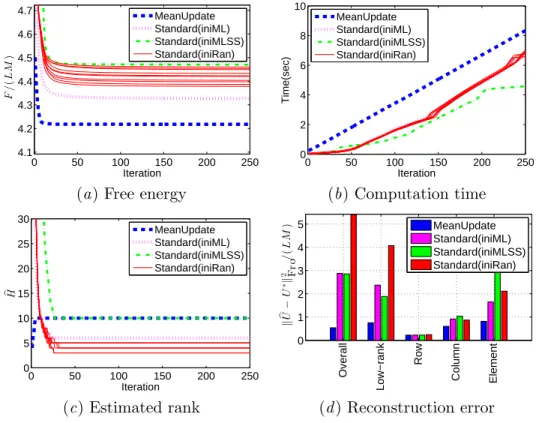
Figure 3: Experimental results with ‘LRCE’-SAMF for an artificial dataset (L = 40, M = 100, H∗ = 10, ρ = 0.05).
We conducted an experiment with artificial data. We assume the empirical VB sce- nario with unknown noise variance, i.e., the hyperparameters {CA(k,s), CB(k,s)}Kk=1,(s)Ss=1 and the noise variance σ2 are also estimated from observations. We use the full-rank model (H = min(L, M )) for the low-rank term Ulow-rank, and expect the MIR effect to find the true rank of Ulow-rank, as well as the non-zero entries in Urow, Ucolumn, and Uelement.
We created an artificial dataset with the data matrix size L = 40 and M = 100, and the rank H∗ = 10 of the true low-rank matrix Ulow-rank∗= B∗A∗⊤. Each entry in A∗ ∈ RM ×H∗ and B∗ ∈ RL×H∗ follows N1(0, 1). The true row-wise (column-wise) part Urow∗ (Ucolumn∗) was created by first randomly selecting ρL rows (ρM columns) for ρ = 0.05, and then adding a noise subject to NM(0, 100 · IM) (NL(0, 100 · IL)) to each of the selected rows (columns). The true element-wise part Uelement∗ was similarly created by first selecting ρLM entries, and then adding a noise subject to N1(0, 100) to each of the selected entries. Finally, an observed matrix V was created by adding a noise subject to N1(0, 1) to each entry of the sum ULRCE∗ of the four true matrices.
It is known that the standard VB iteration (given in Section 4.2) is sensitive to initial- ization (Nakajima et al., 2011). We set the initial values in the following way: the mean parameters { bA(k,s), bB(k,s)}Kk=1,(s)Ss=1were randomly created so that each entry follows N1(0, 1). The covariances {ΣA(k,s), ΣB(k,s)}Kk=1,(s)Ss=1and the hyperparameters {CA(k,s), CB(k,s)}Kk=1,(s)Ss=1were
set to the identity matrix. The initial noise variance was set to σ2= 1. Note that we rescaled V so that ∥V ∥2Fro/(LM ) = 1, before starting iteration. We ran the standard VB algorithm 10 times, starting from different initial points, and each trial is plotted by a solid line (labeled as ‘Standard(iniRan)’) in Figure 3.
Initialization for the MU algorithm (described in Algorithm 1) is simple. We just set initial values as follows: bU(s)= 0L,M for s = 1, . . . , S, and σ2 = 1. Initialization of all other variables is not needed. Furthermore, we empirically observed that the initial value for σ2 does not affect the result much, unless it is too small. Note that, in the MU algorithm, initializing σ2 to a large value is not harmful, because it is set to an adequate value after the first iteration with the mean parameters kept bU(s) = 0L,M. The result with the MU algorithm is plotted by the dashed line in Figure 3.
Figures3(a)–3(c) show the free energy, the computation time, and the estimated rank, respectively, over iterations, and Figure3(d )shows the reconstruction errors after 250 iter- ations. The reconstruction errors consist of the overall error ∥ bULRCE− ULRCE∗∥Fro/(LM ), and the four component-wise errors ∥ bU(s)− U(s)∗∥Fro/(LM ). The graphs show that the MU algorithm, whose iteration is computationally slightly more expensive, immediately converges to a local minimum with the free energy substantially lower than the standard VB iteration. The estimated rank agrees with the true rank bH = H∗ = 10, while all 10 trials of the standard VB iteration failed to estimate the true rank. It is also observed that the MU algorithm well reconstructs each of the four terms.
We can slightly improve the performance of the standard VB iteration by adopting dif- ferent initialization schemes. The line labeled as ‘Standard(iniML)’ in Figure3indicates the maximum likelihood (ML) initialization, i.e, (ba(k,s)h , bb(k,s)h ) = (γh(k,s)1/2ω(k,s)ah , γh(k,s)1/2ω(k,s)b
h ).
Here, γh(k,s) is the h-th largest singular value of the (k, s)-th PR matrix V′(k,s) of V (such that Vl′(k,s)′,m′ = VX(s)(k,l′,m′)), and ω(k,s)ah and ω(k,s)b
h are the associated right and left singu- lar vectors. Also, we empirically found that starting from a small σ2 alleviates the local minima problem. The line labeled as ‘Standard(iniMLSS)’ indicates the ML initialization with σ2 = 0.0001. We can see that this scheme tends to successfully recover the true rank. However, the free energy and the reconstruction error are still substantially worse than the MU algorithm.
We tested the algorithms with other SAMF models, including ‘LCE’-SAMF, ‘LRE’- SAMF, and ‘LE’-SAMF, under different settings for L, M, H∗, and ρ. We empirically found that the MU algorithm generally gives a better solution with lower free energy and smaller reconstruction errors than the standard VB iteration.
We also conducted experiments with benchmark datasets available from UCI repository (Asuncion and Newman, 2007), and found that, in most of the cases, the MU algorithm gives a better solution (with lower free energy) than the standard VB iteration.
5.2. Real-world Application
Finally, we demonstrate the usefulness of the flexibility of SAMF in a foreground (FG)/background (BG) video separation problem. Candes et al. (2009) formed the ob- served matrix V by stacking all pixels in each frame into each column, and applied robust PCA (with ‘LE’-terms)—the low-rank term captures the static BG and the element-wise (or pixel-wise) term captures the moving FG, e.g., people walking through. Babacan et al.
(2012) proposed a VB variant of robust PCA, and performed an extensive comparison that showed advantages of the VB robust PCA over other Bayesian and non-Bayesian robust PCA methods (Ding et al.,2011;Lin et al.,2010), as well as the Gibbs sampling inference method with the same probabilistic model. Since their state-of-the-art method is concep- tually the same as our VB inference method with ‘LE’-SAMF (although the prior design is slightly different), we use ‘LE’-SAMF as a baseline method for comparison.
The SAMF framework enables a fine-tuned design for the FG term. Assuming that the pixels in an image segment with similar intensity values tend to share the same label (i.e., FG or BG), we formed a segment-wise sparse SMF term: U′(k) for each k is a col- umn vector consisting of all pixels within each segment. We produced an over-segmented image of each frame by using the efficient graph-based segmentation (EGS) algorithm (Felzenszwalb and Huttenlocher, 2004), and substituted the segment-wise sparse term for the FG term. We call this method a segmentation-based SAMF (sSAMF). Note that EGS is very efficient: it takes less than 0.05 sec on a laptop to segment a 192 × 144 grey image. EGS has several tuning parameters, to some of which the obtained segmentation is sensitive. However, we confirmed that sSAMF performs similarly with visually different segmentations obtained over a wide range of tuning parameters. Therefore, careful parameter tuning of EGS is not necessary for our purpose.
We compared sSAMF with ‘LE’-SAMF on the ‘WalkByShop1front’ video from the Caviar dataset.1 Thanks to the Bayesian framework, all unknown parameters (except the ones for segmentation) are estimated automatically with no manual parameter tuning. For both models (‘LE’-SAMF and sSAMF), we used the MU algorithm, which has been shown in Section5.1 to be practically more reliable than the standard VB iteration. The original video consists of 2360 frames, each of which is an image with 384 × 288 pixels. We resized each image into 192 × 144 pixels, and sub-sampled every 15 frames. Thus, V is of the size of 27684 (pixels) × 158 (frames). We evaluated ‘LE’-SAMF and sSAMF on this video, and found that both models perform well (although ‘LE’-SAMF failed in a few frames).
To contrast the methods more clearly, we created a more difficult video by sub-sampling every 5 frames from 1501 to 2000 (100 frames). Since more people walked through in this period, BG estimation is more unstable. The result is shown in Figure 4.
Figure 4(a) shows an original frame. This is a difficult snap shot, because the person stayed at the same position for a moment, which confuses separation. Figures4(b)and4(c) show the BG and the FG terms obtained by ‘LE’-SAMF, respectively. We can see that
‘LE’-SAMF failed to separate (the person is partly captured in the BG term). On the other hand, Figures4(e)and 4(f ) show the BG and the FG terms obtained by sSAMF based on the segmented image shown in Figure4(d ). We can see that sSAMF successfully separated the person from BG in this difficult frame. A careful look at the legs of the person makes us understand how segmentation helps separation—the legs form a single segment (light blue colored) in Figure 4(d ), and the segment-wise sparse term (4(f )) captured all pixels on the legs, while the pixel-wise sparse term (4(c)) captured only a part of those pixels.
We observed that, in all frames of the difficult video, as well as the easier one, sSAMF gave good separation, while ‘LE’-SAMF failed in several frames.
1.http://groups.inf.ed.ac.uk/vision/CAVIAR/CAVIARDATA1/
(a) Original (b) BG (‘LE’-SAMF) (c) FG (‘LE’-SAMF)
(d ) Segmented (e) BG (sSAMF) (f ) FG (sSAMF)
Figure 4: ‘LE’-SAMF vs segmentation-based SAMF. 6. Conclusion
In this paper, we formulated a sparse additive matrix factorization (SAMF) model, which allows us to design various forms of factorization that induce various types of sparsity. We then proposed a variational Bayesian (VB) algorithm called the mean update (MU), based on a theory built upon the unified SAMF framework. The MU algorithm gives the global optimal solution for a large subset of parameters in each step. Through ex- periments, we showed that the MU algorithm compares favorably with the standard VB iteration. We also demonstrated the usefulness of the flexibility of SAMF in a real-world foreground/background video separation experiment, where image segmentation is used for automatically designing a SMF term.
Acknowledgments
The authors thank anonymous reviewers for their suggestions, which improved the paper, and will improve its journal version. Shinichi Nakajima and Masashi Sugiyama thank the support from Grant-in-Aid for Scientific Research on Innovative Areas: Prediction and Decision Making, 23120004. S. Derin Babacan was supported by a Beckman Postdoctoral Fellowship.
References
A. Asuncion and D.J. Newman. UCI machine learning repository, 2007. URL http://www.ics.uci.edu/~mlearn/MLRepository.html.
S. D. Babacan, M. Luessi, R. Molina, and A. K. Katsaggelos. Sparse Bayesian methods for low-rank matrix estimation. IEEE Trans. on Signal Processing, 60(8):3964–3977, 2012.