control design for an L-shaped
arm driven by linear motor
Yanfeng Wu
Department of Electronic and Information Engineering
The Graduate School of Engineering
(Doctoral Course)
TOKYO UNIVERSITY
OF AGRICULTURE AND TECHNOLOGY
The guidance and support of the following people are invaluable. I would like to express my sincere appreciation to everyone who helped me scientifically and emotionally throughout my Ph.D study.
Firstly, I would like to express my sincere gratitude to my supervisor Prof. Mingcong Deng, for his continuous support for my Ph.D study and the related research, for his patience, encouragement, and immense knowledge. His insightful guidance has helped me in all the time of research and writing of this dissertation. Without his guidance, it would be impossible to complete this dissertation.
Besides my supervisor, I would like to express my gratitude to this dis-sertation committee: Prof. Yasuhiro Takaki, Prof. Ken Nagasaka, Prof. Toshihisa Tanaka and Prof. Kenta Umebayashi, their insightful comments, valuable suggestions incent me to widen my research from various perspec-tives.
In this dissertation, the operator-based robust nonlinear vibration control is proposed for an L-shaped arm driven by a linear pulse motor. The aim of this study is to allow the motor move fast and reduce the arm vibration by controlling the motion of the motor and the behaviour of the piezoelectric actuator simultaneously.
Much manipulating devices in the industrial system are constructed with flexible arms and driven by motors. When the system works, the vibration of the arm will degrade the system performance. To control the vibrations, there are mainly two active ways. One way is controlling the motor motion such that the vibrations are reduced. Another way uses smart materials as actuator on the flexible arms to suppress the vibrations. In this dissertation, the L-shaped arm pasted with a piezoelectric actuator is driven by a linear pulse motor. It is difficult to control the linear motor and the piezoelec-tric actuator at same time to meet all the requirements, while the system has uncertainties and hysteresis nonlinearities. The operator-based nonlin-ear control approach is effective and easy implemented for these nonlinnonlin-ear systems. Therefore, two robust nonlinear controls based on the nonlinear operator control theory are designed to control the motor motion and the behavior of the piezoelectric actuator simultaneously, such that the motor moves fast while the arm vibration is reduced as much as possible.
can-uncertainties which are compensated in the control design. Prandtl-Ishlinskii model is utilized to model the behaviour of the piezoelectric actuator. The model is divided into two parts, one part is linear to be combined into the operator among the control design; the residual part including the hystere-sis is to be compensated in the tracking controller such that the stability of the system is guaranteed. Based on the operator-based nonlinear control approach, two controllers are designed to control the system in parallel. One controller controls the motor motion in optimal trajectory while reducing the arm vibration. Another one controls the behaviour of the piezoelectric actuator such that the arm vibration is further reduced. The hysteresis non-linearity of the actuator is compensated in a tracking controller. Simulations are conducted in Matlab comparing with the Proportional-Integral (PI) con-trol to confirm the effectiveness of the proposed concon-trol design. The results illustrate that the operator-based control systems designed in this disserta-tion is effective to reduce the arm vibradisserta-tion while control the motor modisserta-tion in less time and can guarantee robust stability of the system.
controller. The operator-based right coprime factorization method is utilized to guarantee the robust stability of the motor-arm system. The piezoelectric actuator is controlled to further reduce the arm vibration. With a modified compensator, the hysteresis of the piezoelectric actuator is compensated in the control design by using a Prandtl-Ishlinskii hysteresis model. The load is estimated by DWT and fast Fourier transform (FFT) method based on the relationship between vibration model of the L-shaped arm and the mass of load, such that the main parameters of the system dynamic is determined. The DWT is used to decompose the arm vibration signal and extract the first mode of the arm vibration, FFT is then used to transform the arm vibration signal from time domain into frequency domain. Simulation results compar-ing with previous control are demonstrated to validate performance of the proposed control design. The results show that the on-line DWT is effective to remove the influence of some uncertainties and improve the performance of the operator-based control; the load estimation method is workable.
improved and the load mass is estimated.
1 Introduction 1
1.1 Background . . . 1
1.2 Current development of arm vibration control . . . 3
1.3 Motivations of the dissertation . . . 6
1.4 Contributions of the dissertation . . . 8
1.5 Organization of the dissertation . . . 10
2 Preliminaries and problem statement 13 2.1 Introduction . . . 13
2.2 Flexible arm vibration model . . . 14
2.3 Model of piezoelectric actuator . . . 15
2.4 Operator-based nonlinear control approach . . . 17
2.4.1 Definitions of spaces . . . 17
2.4.2 Definitions of operators . . . 18
2.4.3 Right coprime factorization . . . 21
2.5 Fundamental theories on discrete wavelet transform . . . 25
2.5.1 Wavelet transform . . . 25
3 Operator-based control design for the L-shaped arm without
load 31
3.1 Introduction . . . 31
3.2 Model of the L-shaped arm vibration . . . 32
3.3 Proposed robust nonlinear control design . . . 36
3.3.1 Control scheme for the Arm-Motor system . . . 36
3.3.2 Operator-base system representation . . . 37
3.3.3 Optimal control for the linear pulse motor . . . 39
3.3.4 Control system for Arm 2 vibration with piezoelectric actuator . . . 42
3.4 Simulation results and discussion . . . 45
3.5 Conclusion . . . 50
4 Operator-based control design for the L-shaped arm with unknown load 55 4.1 Introduction . . . 55
4.2 Modelling of the system with load . . . 56
4.2.1 Model of arm vibration with load . . . 56
4.2.2 Load estimation method . . . 59
4.3 On-line wavelet transform . . . 61
4.4 Operator-based control design with DWT . . . 63
electric actuator . . . 68
4.5 Numerical simulations and discussion . . . 71
4.5.1 The modified contol without DWT . . . 71
4.5.2 Operator-based control with DWT . . . 72
4.6 Conclusion . . . 78
5 Experimental study on the control design 83 5.1 Introduction . . . 83
5.2 Experiment system structure . . . 84
5.3 Experiments on system without load . . . 86
5.4 Experiments on system with load . . . 91
5.5 Conclusion . . . 96
6 Conclusions 99 Bibliography 103 Appendix A Model analysis of the L-shaped arm with load 119 A.1 Free vibration of the arm . . . 119
A.2 Free vibration of the L-shaped arm . . . 121
A.3 Forced vibration due to initial conditions . . . 125
2.1 Transverse vibration of a uniform thin arm . . . 14
2.2 Right factorization of a nonlinear plant . . . 22
2.3 Right coprime factorization of a nonlinear plant . . . 22
2.4 Nonlinear feedback control system with uncertainties . . . 24
2.5 DWT processing scheme . . . 26
3.1 Schematic diagram of L-shaped arm system . . . 32
3.2 Proposed control scheme . . . 36
3.3 Proposed control loop structure . . . 37
3.4 The proposed control flowchart . . . 38
3.5 Operator-based control system for linear motor . . . 41
3.6 Control scheme for Arm 2 vibration . . . 43
3.7 Equivalent control system with hysteresis compensator . . . . 44
3.8 Displacement of Arm 1 with and without feedback control . . 47
3.9 Position and speed of motor (with PI control) . . . 48
3.13 Displacement of Arm 2 without and with actuator control
(without hysteresis compensation) . . . 52
3.14 Control input for actuator without hysteresis compensation . . 52
3.15 Displacement of Arm 2 without and with hysteresis compen-sation . . . 53
3.16 Control input for actuator with hysteresis compensation . . . 53
4.1 System structure . . . 57
4.2 The sketch of the L-shaped arm . . . 58
4.3 The relationship between the first mode frequency and load mass . . . 60
4.4 On-line DWT processing flow . . . 62
4.5 Nonlinear operator-based robust control with DWT . . . 63
4.6 Proposed control scheme for the arm with load . . . 64
4.7 Proposed control flow chart . . . 65
4.8 Operator-based linear motor motion control using DWT . . . 67
4.9 Operator-based control for Arm 2 with DWT considering hys-teresis . . . 70
4.10 Vibration of Arm 1 with and without control . . . 72
4.11 Vibration of Arm 1 with new model . . . 73
4.12 Vibration of Arm 2 with and without control . . . 74
4.16 Position and speed of the linear motor . . . 78
4.17 Vibration of Arm 1 with and without control . . . 79
4.18 Vibration control of Arm 1 with and without DWT . . . 80
4.19 Vibration of Arm 2 with piezoelectric actuator . . . 80
4.20 Vibration of Arm 2 with and without compensation . . . 81
4.21 Robustness of the proposed control . . . 81
5.1 Experimental device . . . 84
5.2 Schematic diagram of the arm . . . 85
5.3 Vibration of Arm 1 with motion control (without piezoelectric actuator) . . . 87
5.4 Vibration of Arm 2 with and without actuator (linear motor with operator control) . . . 89
5.5 Cumulative vibration intensity of Arm 2 with and without actuator . . . 90
5.6 Robustness of the proposed system . . . 91
5.7 Position and force input of the linear motor . . . 93
5.8 Vibration of Arm 1 with and without control . . . 94
5.9 Vibration of Arm 1 with and without DWT . . . 95
5.10 Vibration of Arm 1 with and without control . . . 96
5.11 Vibration of Arm 1 with and without DWT . . . 97
3.1 Some parameters of the L-shaped Arm . . . 45
3.2 Parameters of the linear pulse motor . . . 46
4.1 Load mass estimation in simulation . . . 73
5.1 Parameters of the Piezoelectric Actuator . . . 85
Introduction
1.1
Background
sen-sors to feed back the real time vibration states and reducing the unwanted vibration by the anti-force generated by powered actuators [3–6].
The traditional actuating components usually use pneumatic devices, lin-ear motors, electromagnetic devices etc. in vibration control. Thanks to the reciprocal physical characteristic of smart materials including magnetostric-tive materials, shape memory alloys and piezoelectric materials etc., they are much commonly used in modern engineering to suppress the structural vibrations. Among them, piezoelectric material is one kind of such materials that produces strain and stress when voltages are applied, and vice versa. Therefore, it has been utilized as sensors and actuators and being studied by much researchers [7–9].
has become more comprehensive and effective. It has been used in many practical applications [19–24].
The wavelet transform can convert the signal into time-scale domain, has attracted increasing attentions for its ability to extract signal features [25–30]. Wavelet transform has been extended to civil engineering, machining condition monitoring and detection [31–33]. However, most approaches are off-line precess or need the whole length of signals, which limits its on-line applications for time control. Some researchers propose on-line or real-time segmented wavelet transform applying for wheel system, rotor and other rotational machines [34–38].
1.2
Current development of arm vibration
con-trol
the rotation and translation of the rotational-translational actuator systems influenced by nonvanishing matched disturbances [76]. In this study, the whole system is a Multi-Input Multi-Output (MIMO) plant. For the MIMO nonlinear plants, some operator-based approaches are proposed for tackling the coupling problem in [53–56]. However, these plants have the same number of inputs as outputs, not suitable for the plants with unequal inputs and outputs.
utilized to describe hysteresis nonlinearity using stop hysteresis operators or play hysteresis operators because of its simplicity, accuracy and ease of im-plementation. However, these operators are symmetric, which will still result in compensation error. Al Janaidehet al[82] proposed an analytic inverse of a generalized Prandtl-Ishlinskii model, it can be conveniently implemented as a real-time feed-forward compensator to compensate for hysteresis nonlin-earities. A non-symmetric Prandtl-Ishlinskii hysteresis model with unknown slopes was given to describe the hysteresis in [73], the nonlinear compensator based on this model can compensate the hysteresis more effectively.
An operator-based nonlinear control method has been given to control the vibration of a flexible arm using the piezoelectric actuator [86]. However that paper only studied the free vibration of a simple uniform clamped-free beam and without considering the hysteresis of actuator. For controlling the free vibration of an aircraft-tail-like plate using the piezoelectric actua-tor, an operator-based nonlinear system control technique has been given by Katsurayama et al. [74], the lower order modes of vibration are considered. However, that study only considered the free vibration the plate without driving source control.
sliding-mode control, fuzzy control and optimal control. Wenet al. [52] used data-based support vector machine (SVM) to estimate the swing angle, found an optimal trajectory to reduce the payload swing using operator-based con-trol. However the control object in that paper is a payload driven by a linear motor with cable, the swaying of the payload is much more slowly and quite different from the arm vibration. As the L-shaped arm has a more compli-cated vibration dynamics, it is difficult for the SVM to learn. Therefore the control method in that paper is not suitable for this L-shaped arm vibration.
1.3
Motivations of the dissertation
Scaled down from a real industrial transported system, a flexible L-shaped arm driven by a linear pulse motor is studied in this dissertation. When the system is working, vibration of the arm is inevitable. It is necessary to seek appropriate methods to control the motor motion while reduce the arm vibration at the same time.
Motivated by the optimal motor motion control for the underactuated system, this dissertation intend to set up an optimal control method for the linear motor. The motor is controlled with optimal trajectory resulting in less time consumption and less arm vibration. It means that the arm vibration status will be measured by sensors and feed back into the motor motion control. The main difficulty is to meet two output requirements with one control input while keep the system stable and robust.
measure and suppress the arm vibration. Prandtl-Ishlinskii model is used to model the hysteresis of the piezoelectric actuator and modify it accord-ing to the control design method, its nonlinearity will be considered to be compensated to improve the control performance.
system. The on-line DWT is constructed to estimate the unknown load, re-move the influence of some uncertainties and improve the performance of the operator-based control.
In summary, this dissertation intend to use operator-based nonlinear con-trol approach and on-line DWT in concon-trol design for actively concon-trol the L-shaped arm vibration system, and validate the control design in simulation and experiment. The aim of this research is to allow the motor move fast and reduce the arm vibration as much as possible while keep the system stable and robust.
1.4
Contributions of the dissertation
For the L-shaped arm experiment system control design, the difficulty is controlling the linear motor and the piezoelectric actuator at same time to meet all the requirements, while the system has uncertainties and hysteresis nonlinearities. We design two controllers based on the nonlinear operator control theory to accomplish it. One controller allows the fast movement to destination while reducing the vibration of the arm, the other one con-trols the piezoelectric actuator to further reduce the vibration. The main contributions of this study are summarized as follows.
(1) The vibration of the Motor-Arm system with and without
load is modelled.
dimen-sional Euler beam by mechanical analysis based on Euler-Bernoulli theory, and the relationship between the load and the vibration mode is given. By introducing a evaluation index, the dominant modes of the arm vibration are considered in the control design, other higher modes are considered as uncertainties compensated in the control design.
(2) The load estimation method is given by using DWT and
FFT.
Based on the vibration model of the L-shaped arm with load, the relation-ship between the load mass and the natural frequency of the arm vibration is obtained. When the arm vibration is measured in time domain signal, after decomposing by the DWT, the first mode vibration is isolated and transformed into frequency domain by FFT. The load is estimated using the obtained relationship, such that the main parameters of the system dynamic is determined.
(3) Two operator-based nonlinear controllers for motor motion
and arm vibration are designed employing a short-symmetrical
on-line DWT.
1.5
Organization of the dissertation
Beginning with theoretical preliminaries and problem statement, this disser-tation is organized as follows.
In Chapter 2, some fundamental definitions and the theoretical basis are provided for the system modelling and control design in this dissertation. Euler-Bernoulli beam theory is utilized to model the flexible arm vibration; Prandtl-Ishlinskii model is used to model the hysteresis of the piezoelectric actuator. Some fundamental definitions of operator theory are introduced, the operator-based nonlinear control approach and the discrete wavelet trans-form are given. Based on the background and these theories, the problem to be studied in this dissertation is stated.
In Chapter 3, the forced vibration of the L-shaped arm driven by a linear pulse motor is modelled by considering it as two connected Euler-Bernoulli beams. Based on the operator-based nonlinear control approach, two controllers are designed to control the system in parallel. One controller aims to control the motor motion in optimal trajectory while reducing the arm vibration. Another one aims to control the behaviour of the piezoelectric actuator to further reduce the arm vibration. The hysteresis nonlinearity of the actuator is compensated in a tracking controller. Simulation is conducted to confirm the effectiveness of the proposed control design.
im-prove the performance of the operator-based control. Involving the on-line DWT, two operator-based controllers are proposed. One is to control the mo-tor motion resulting in less arm vibration. Another one is to further reduce the arm vibration by using a piezoelectric actuator. Simulations comparing with previous control are demonstrated to validate performance of the pro-posed control design. The load estimation method using FFT and DWT is given based on the system model.
InChapter 5, the structure of the L-shaped arm vibration experimental system is introduced, the main parameters of the devices are identified. Using the operator-based nonlinear optimal control proposed in Chapter 3, exper-iments are conducted comparing with the conditional PI control to test the experimental performance of the control design. Using the operator-based nonlinear control with on-line DWT proposed in Chapter 4, comparative ex-periments are conducted for the L-shaped arm with unknown load to validate the load estimation method and test the performances of the control designs correspondingly.
Preliminaries and problem
statement
2.1
Introduction
This chapter provides the mathematical and theoretical basis for the system modelling and control design in the following chapters of this dissertation. It also specify the aims and objectives of this research.
InSection 2.2, the dynamics of flexible arm vibration is introduced, and its modelling method based on Euler-Bernoulli beam theory is provided.
InSection 2.3, the dynamics of the piezoelectric actuator is introduced, the hysteresis of the piezoelectric actuator is modelled using a Prandtl-Ishlinskii hysteresis model.
InSection 2.4, the fundamental definitions of operator theory are intro-duced, the operator-based nonlinear control approach is outlined.
In Section 2.5, the theoretical basis of wavelet transform is given, some related definitions of DWT is introduced.
Primarily, the framework of modelling the L-shaped arm vibration and hys-teresis of the piezoelectric actuator, operator-based control design utilizing DWT is outlined.
2.2
Flexible arm vibration model
If a thin uniform arm has external distributed transverse force q(x, t) on it, shown as in Fig. 2.1(a), take any element of the beam with length dx as object, its free-body diagram is shown in Fig. 2.1(b), where V(x, t) is the shear force, M(x, t) is the bending moment, ρ is the mass density.
Figure 2.1: Transverse vibration of a uniform thin arm
[77], force and moment equilibrium, the forced transverse vibration of the uniform arm is obtained as:
EaI ∂4w
∂x4 +csI
∂5y(x, t)
∂x4∂t +ρS
∂2w
∂t2 =q(x, t) (2.1)
whereq(x, t) is the external distributed forces on the arm, including the linear motor driving force and the piezoelectric actuator moment. w, standing for
w(x, t), is the transverse displacement along the neutral axis of the arm.
Ea, I, ρ, S, cs are the Young’s modulus, moment of inertia, density,
cross-sectional area and strain-rate damping coefficient of the arm, respectively. The equation (2.1) can be solved using the boundary conditions and the arm’s initial conditions.
2.3
Model of piezoelectric actuator
imple-mentation. To consider this effect in the system model, in this dissertation, the Prandtl-Ishlinskii hysteresis model based on the play hysteresis operator is utilized, represented as follows.
Mp(t) =DP I(u)(t) + ∆P I(u)(t) (2.2)
The output of piezoelectric actuator is represented as two terms. The first term DP I is an invertible operator for certain parameters, the residual term
∆P I is the nonlinear part of the model, which will change with the inputu(t)
and be influenced by the design parameters, it needs to be compensated by the controller. The details ofDP I and ∆P I are shown as follows.
DP I(u(t)) =Ku(t) =u(t)
∫ H
0
p(h)dh, (2.3)
∆P I(u(t)) =−
∫ hx
0
Snhp(h)dh+
∫ H
hx
p(h)[Fh(u(ti))−u(t)]dh, (2.4)
Sn =sign(u(t)−Fh(u(ti)))
Fh(u(t)) =
u(t) +h u(t)≤Fh(u(ti))−h Fh(u(ti)) −h < u(t)−Fh(u(ti))< h u(t)−h u(t)≥Fh(u(ti)) +h
ti < t≤ti+1, 0≤i≤N −1 (2.5)
0 =t0 < t1 <· · ·< tN =tE, [0, tE].
where, u(t) and h are the input voltage and the threshold of play hys-teresis operator, respectively. The initial condition is given by Fh(u)(0) =
max(u(0)−h,min(u(0) +h,(u1)∗). hx is the upper limit of h that satisfies h ≤ |u(t)−Fh(u(ti))|. p(h) is the density function satisfying p(h)≥ 0 with
∫∞
2.4
Operator-based nonlinear control approach
2.4.1
Definitions of spaces
In this dissertation, the operator theory is based on several spaces in math-ematics, which are defined as follows.
Normed linear space:
Denote a space X of time functions, it is said to be a vector space if it is closed under addition and scalar multiplication. It is said to be normed
if each element x in X is endowed with norm ∥ · ∥X, satisfying the follow
conditions:
1) ∥x∥>0, if x̸= 0.
2) ∥ax∥=|a|∥x∥.
3) ∥x1+x2∥ ≤ ∥x1∥+∥x2∥.
Banach space:
A Banach space is a vector space X over the real or complex numbers with a norm ∥ · ∥ such that every Cauchy sequence (with respect to the metric
d(x, y) = ∥x −y∥) in X has a limit in X. Many spaces of sequences or functions are infinite dimensional Banach spaces.
Extended linear space:
Pro-jection operator mapping fromZ to another linear space, ZT, of measurable
functions such that
fT(t) := PT(f)(t) =
{
f(t), t≤T
0, t > T (2.6)
where, fT(t)∈ ZT is called the truncation of f(t) with respect to T. Then,
for any given Banach spaceX of measurable functions, if
Xe ={f ∈Z : ∥fT∥X <∞,for all T <∞}, (2.7)
the space Xe is called the extended linear space associated with the Banach
space X.
This dissertation uses the extended linear space because the control sig-nals are finite time-duration in experiments.
2.4.2
Definitions of operators
Let U and Y be linear spaces over the field of real numbers, and let Us
and Ys be normed linear subspaces, called the stable subspaces of U and Y,
respectively.
Operator:
An operator Q : U → Y is a mapping defined from input space U to the output space Y. The operator Q can be expressed as y(t) =Q(u)(t) where
u(t) is the element of U and y(t) is the element ofY.
Invertible:
An operatorQis said to be invertible if there exists an operator P such that
P is called the inverse of Q and is denoted by Q−1, where, I is identity
operator, and Q◦P (or simplyQ(P(·)) or QP) is an operation satisfying
D(Q◦P) =P−1(
R(P)∩ D(Q)). (2.9)
Unimodular operator:
Let S(U, Y) be the set of stable operators mapping from U to Y. Then, S(U, Y) contains a subset defined by
U(U, Y) = {M :M ∈ S(U, Y), M is invertible with M−1 ∈ S(Y, U)}.(2.10)
Elements of U(U, Y) are called unimodular operators.
Lipschitz operator:
For any subset D ⊆U, let F(D, Y) be the family of nonlinear operators Q
such thatD(Q) =Dand R(Q)⊆Y. Introduce a (semi)-norm into (a subset of) F(D, Y) by
∥Q∥ := sup
x,x˜∈D x̸= ˜x
Q(x)−Q(˜x)
Y
∥x−x˜∥U
if it is finite. In general, it is a semi-norm in the sense that ∥Q∥ = 0 does not necessarily implyQ= 0. In fact, it can be easily seen that∥Q∥= 0 if Q
is a constant operator (need not to be zero) that maps all elements from D
to the same element in Y.
operator Q on D. A Lipschitz operator is bounded and continuous on its own domain.
Generalized Lipschitz operator:
Let Ue and Ye be extended linear spaces associating respectively with two
given Banach spaces U and Y of measurable functions defined on the time domain [0,∞), and letDbe a subset ofUe. A nonlinear operatorQ:D→Ye
is called a generalized Lipschitz operator on D if there exists a constant L
such that
[Q(x)]T −[Q(˜x)]T
Y ≤L∥xT −x˜T∥U (2.11)
for all x,x˜∈ D and for all T ∈ [0,∞). Note that the least such constant L
is given by the norm of Q with
∥Q∥Lip:= ∥Q(x0)∥Y +∥Q∥
= ∥Q(x0)∥Y
+ sup
T∈[0,∞)
sup
x,x˜∈D xT̸= ˜xT
[Q(x)]T −[Q(˜x)]T
Y
∥xT −x˜T∥U
(2.12)
for any fixedx0 ∈D.
Based on (2.12), it follows immediately that for any T ∈[0,∞)
[Q(x)]T −[Q(˜x)]T
Y ≤ ∥Q∥∥xT −x˜T∥U
≤ ∥Q∥Lip∥xT −x˜T∥U. (2.13)
Lemma 2.1Let Ue andYe be extended linear spaces associating respectively
of Ue. The following family of Lipschitz operators is a Banach space: Lip(D, Ye) =
{
Q:D→Ye∥Q∥Lip <∞ onD }
. (2.14)
Bounded input bounded output (BIBO) stability:
LetQbe a nonlinear operator with its domainD(Q)⊆Ueand rangeR(Q)⊆ Ye. If Q(U) ⊆ Y, Q is said to be input output stable. If Q maps all input
functions fromUs into the output spaceYs, that isQ(Us)⊆Ys, then operator Q is said to be bounded input bounded output (BIBO) stable or simply, stable. Otherwise, if Q maps some inputs from Us to the set Ye\Ys (if not
empty), then Q is said to be unstable. For any stable operators defined following in this dissertation stands for BIBO stable.
2.4.3
Right coprime factorization
Represent a nonlinear time varying system with uncertainties as operator
P + ∆P : U → Y. Where P is the nominal plant, ∆P stands for the uncertainties, U and Y denote the input and output space of the plant.
Right factorization:
By introducing an intermediate variable ω ∈ W, W is called a quasi-state space of P, the input and output of the operator P are expressed as y =
N(ω) and u = D(ω). If D is invertible, ω(t) =D−1(u)(t) , then P(u)(t) =
N(ω)(t) = N D−1(u)(t); if further N and D are two stable operators, the
Figure 2.2: Right factorization of a nonlinear plant
Right coprime factorization:
After right factorization of a plant P into (N, D), if two operators A and
B satisfy the following Bezout identity, the factorization is said to be right coprime factorization.
AN +BD=M (2.15)
Where B is invertible and M ∈ U(W, U) is a unimodular operator. The block diagram of the right coprime factorization of a nonlinear system P
is shown in Fig. 2.3. Fig. 2.3 is therefore to be said as a operator-based
Figure 2.3: Right coprime factorization of a nonlinear plant
feedback control for the nonlinear plant P, and the operatorsAand B serve as controllers.
dissertation,t0 = 0 andw0 =w0(t0) are selected.
Well-posedness:
The feedback control system shown in Fig. 2.3 is said to be well-posed, if for every input signal r∈U, all signals in the system (i.e., e, u,w, b and y) are uniquely determined.
Overall stable:
The feedback control system shown in Fig. 2.3 is said to be overall stable, if
r∈Us, implies that u∈Us, y∈Vs, w∈Ws, e∈Us and b ∈Us.
Lemma 2.2 Assume that the system shown in Fig. 2.3 is well-posed. If the system has a right factorizationP =N D−1, then the system is overall stable
if and only if the operator M in (2.15) is a unimodular operator. Robustness:
For a nonlinear plat ˜P, it is represented as a nominal plant P and bounded uncertainty ∆P, and ˜P = P + ∆P. The right factorization of the nominal plan P and the overall plant ˜P are
P =N D−1 (2.16)
and
P + ∆P = (N + ∆N)D−1 (2.17)
the following Bezout identity is satisfied,
A(N + ∆N) +BD= ˜M (2.18)
and ˜M is a unimodular operator, the the nonlinear feedback control system is said to be BIBO stable.
With the determined operators A and B, if they further satisfy the fol-lowing condition,
∥[A(N + ∆N)−AN]M−1∥Lip <1 (2.19)
then the robustness of the uncertain system is guaranteed, where ∥ · ∥Lip is
a Lipschitz operator norm. The robust feedback control system is shown in Fig. 2.4.
Figure 2.4: Nonlinear feedback control system with uncertainties
Lemma 2.3 Let Ue
s be a linear subspace of the extended linear space Ue
associated with a given Banach space UB, and let(A(N−∆N) +AN)M−1 ∈ Lip(Ue
s). With the Bezout identity of the nominal plant and the overall plant AN +BD=M ∈ U(W, U), A(N+ ∆N) +BD= ˜M, respectively. If
∥(A(N + ∆N)−AN)M−1∥<1 (2.20)
then the system shown in Fig. 2.4 is said to be robust stable.
2.5
Fundamental theories on discrete wavelet
transform
2.5.1
Wavelet transform
Wavelet transform is performed by using wavelet functions for time domain signal, the wavelet function is usually expressed in the following form.
Ψa,b=
1 √
bΨ( t−a
b ) (2.21)
Where a is the shifting parameter and b is the scaling parameter.
For a time domain signal x(t), the one-dimensional continuous wavelet transform (CWT) is a convolution of x(t) and the complex conjugate of a wavelet function, which can be expressed as follows.
cwt(a, b) = √1
b
∫
x(t)Ψ∗(t−a
b ) (2.22)
where Ψ∗(
·) is the complex conjugate of a wavelet function Ψ(·).
2.5.2
Discrete wavelet transform
CWT need a large amount of computation and resources, which is not suit for the control in practice. It is needed to transit from CWT to discrete wavelet transform (DWT). By insinuate the parametersaandb with a dyadic scales, the DWT is changed in the follow form.
ψm,k(t) = 2−m/2ψ(2−mt−k) (2.23)
high-pass filter h. A sampled signal x is decomposed by passing the filters. At one certain decompose level, the outputs giving the detail coefficients (from the high-pass filter) and approximation coefficients (from the low-pass) as follows.
ylow[n] =
∑
n
x[k]g[2n−k]
yhigh[n] =
∑
n
x[k]h[2n−k] (2.24)
The number of decomposition levels are decided by the frequency band of every level and the frequency frequency of desired signal. The frequency band for the approximation ACj and the detail DCj at level j are given by
0≤fACj ≤ fs
2j+1
fs
2j+1 ≤fDCj ≤ fs
2j
(2.25)
where j is the wavelet decomposition level, fs is the signal sampling
fre-quency. If the reconstruction level is determined by (2.25), by selecting the gains Ka1, Kdj (j = 1,2,· · · , L), the processed signal is reconstructed, as
shown in Fig. 2.5.
2.6
Problem statement
In this dissertation, the L-shaped arm pasted with a piezoelectric actuator is driven by a linear pulse motor. The motor is required to move to desti-nation with less time consuming, while the arm vibration is required to be reduced as much as possible. The difficulty is controlling the linear motor and the piezoelectric actuator at same time to meet all the requirements, while the system has uncertainties and hysteresis nonlinearities. Moreover, if the arm has different loads, the mass of load will impact the system dynamics, therefore, the load mass is required to be determined before control.
There-fore, one of the objectives is how to design an optimal controller to control this underactuated system such that the motor move fast in a optimal tra-jectory, the arm results in less vibration, while keep the system stable and robust.
Secondly, motivated by the superior advantages of the piezoelectric ma-terial, this dissertation intend to use piezoelectric material as sensors and ac-tuator, to measure and suppress the arm vibration. Prandtl-Ishlinskii model is used to model the hysteresis of the piezoelectric actuator and modify it according to the control design method. The main difficulty is how to use the model and design controller to compensate the hysteresis of the piezoelectric actuator.
Thirdly, motivated by the superior advantages of the operator-based non-linear control method, this dissertation intend to utilize the method to fac-torize the system model and design optimal controllers to control the linear motor motion and reduce the L-shaped arm vibration at the same time. The system has two control inputs including driving force of linear pulse motor and voltage for the piezoelectric actuator, three outputs including the mov-ing distance of linear motor and the vibrations of two parts of arm. The main difficulty is how to design the two controllers working together to meet the system requirements.
be processed by appropriate measures, wavelet transform can undertake such tasks. An on-line DWT is to be proposed to use in the operator-based non-linear control, working together for the nonnon-linear L-shaped arm vibration system. Operator-based right coprime factorization method is used to guar-antee the robust stability of the system. The on-line DWT is constructed to estimate the unknown load, remove some uncertainties and improve the performance of the operator-based control.
In summary, this dissertation intend to use operator-based nonlinear con-trol approach and on-line DWT in the concon-trol design for actively concon-trol the L-shaped arm vibration system, and validate the control design in simulation and experiment. The aim of this research is to allow the motor move fast and reduce the arm vibration as much as possible while keeping the system to be robust stable.
2.7
Conclusion
Operator-based control design
for the L-shaped arm without
load
3.1
Introduction
To address the problems mentioned in Chapter 2, in this chapter, the dy-namics on L-shaped arm vibration involving linear motor and piezoelectric actuator is modelled, controls for the motor motion and arm vibration are designed.
In Section 3.2, the vibration of the L-shaped arm is modelled by con-sidering it as two connected Euler-Bernoulli beams, the relationship between the arm vibration and linear motor, piezoelectric actuator is given.
actuator to further reduce the arm vibration. The hysteresis nonlinearity of the actuator is modelled using a Prandtl-Ishlinskii hysteresis model, and the nonlinear part is compensated in the tracking controller.
In Section 3.4, simulation is conducted using the experimental data and comparing with the PI control, the results are shown to confirm the effectiveness of the proposed control design.
In Section 3.5, the conclusion of this chapter is given.
3.2
Model of the L-shaped arm vibration
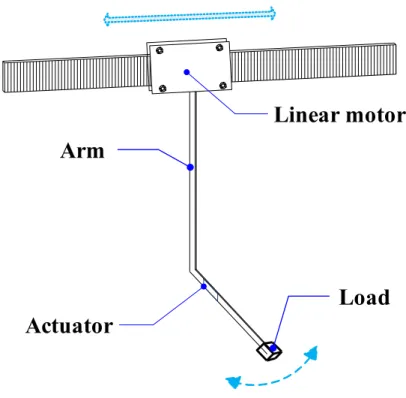
In this dissertation, the L-shaped arm driven by a linear pulse motor which running along the horizontal motor guide is studied, the schematic diagram of the system is shown in Fig. 3.1. When the motor starts running, the arm will unavoidably vibrate.
Figure 3.1: Schematic diagram of L-shaped arm system
part and Arm 2 for horizontal part. The arm is connected with the motor, when the motor moves, the acceleration or deceleration will cause vibration of the arm. In addition, the transient vibration of motor and the uneven friction between the motor and guide will cause the arm additional vibration. In this chapter, the influences beside the acceleration of the motor will be considered as uncertainties or disturbances of the plant. The transverse vibration of Arm 1 is subjected to the excitation of linear pulse motor, and the Arm 2 subjected to the excitation from Arm 1, both are seen as clamped-free Euler-Bernoulli beams [77]. When modelling the vibration of Arm 1, the Arm 2 is considered as a tip mass at the free end. The excitation on Arm 2 depends on the relative transverse vibrations of Arm 1. Neglecting the external damping factor, only considering the strain-rate damping, the vibration of the arm is represented as
ρS∂
2y
i(x, t)
∂t2 +EaI
∂4y
i(x, t) ∂x4 +csI
∂5y
i(x, t)
∂x4∂t =qi(x, t) (3.1)
where yi(x, t) is the transverse displacement relative to the clamped end of
the arm along neutral axis, qi(x, t) is external distributed force on the arm, i(i= 1,2) is the order number representing for Arm 1 and Arm 2. ρ, S, Ea, I
and cs are density, cross-sectional area, Young’s modulus, moment of inertia
and strain-rate damping coefficient of the arm, respectively. The external force on Arm 1 is represented as
q1(x, t) = −
[
ρS+m2δ(x−L1)
]
F01(t)
m1+m2
(3.2)
whereδ(·) is the Dirac delta function,F01(t) is the force from the linear motor
Remark 3.1: In Equation (3.2), the linear motor driving force F01 is an
equivalent term, because the linear motor used in the experimental system is controlled using the speed mode. The certain level friction between slider and stator does not influence the motor motion, unless it exceeds the output range of the motor.
The external forces on Arm 2 include the force from Arm 1 and the moment from the piezoelectric actuator, it is represented as
q2(x, t) =−
F12(t)
L2
+Mp ∂2
∂x2[H(x−xp2)−H(x−xp1)] (3.3)
where F12(t) is the equivalent force from Arm 1 driving Arm 2, Mp is the
moment generated by the piezoelectric actuator. H(·) is a Heaviside function,
xp1,xp2 are positions of the piezoelectric actuator on Arm 2.
Considering the boundary conditions of the arm, based on the expansion theorem, the solutions of Equation (3.1) are obtained as
y1(x, t) =
∞
∑
m=1
J1m(x)
∫ t
0
[
e−αm1(t−τ)sinωm
1d(t−τ)f1mu1(τ)
]
dτ, (3.4)
y2(x, t) =
∞
∑
m=1
J2m(x)
∫ t
0
[
e−αm2(t−τ)sinωm
2d(t−τ)(f2mF12(τ) +f3mu˜2(τ))
]
dτ.
(3.5)
where m(m = 1,2,3,· · ·) is the vibration mode order, u1(t) = F01(t) is the
piezoelectric actuator. fm
i are coefficients relative to the external forces.
f1m =− 1
m1+m2
[
ρS
∫ l1
0
Φm1 (x)dx+m2Φm1 (l1)
]
f2m =−
1
L2
∫ L2
0
Φm2 (x)dx
f3m = ∂Φ
m
2 (xp2)
∂x −
∂Φm
2 (xp1)
∂x
F12 =m2
∂y2 1(l1, t)
∂t2
Other parameters in Equations (3.4) and (3.5) are expressed as follows.
Jm i (x) =
Φm i (x) ωm
id
, ωm
i = ( λm
i Li
)2
√
EaI ρS ,
ζim = csω
m i
2E , ω
m id =ωim
√
1−ζm i 2,
αmi =ζimωim, cs =cmEa.
where Φm
i (x) is the mass normalized eigenfunction of the clamped-free arm
for the m-th mode [77]. ωm
i is the undamped natural frequency of the m-th
mode, ωm
id is the damped natural frequency, σim is the damping ratio. The
dimensionless frequency parameter of the m-th mode λm
i could be obtained
from the corresponding characteristic equations. The details about the vi-bration model arm with load are shown in Appendix A.
3.3
Proposed robust nonlinear control design
3.3.1
Control scheme for the Arm-Motor system
In the whole plant of the L-shaped arm system, there are three outputs and two inputs. By controlling the linear pulse motor and the piezoelectric ac-tuator, Arm 1 and Arm 2 track the reference trajectories. In addition, the piezoelectric actuator and the arm vibration coupling with unknown distur-bances from the motor are both nonlinear systems. To guarantee the robust stability of the system, in this dissertation, we design two controllers based on operator theory, the control scheme is shown in Fig. 3.2.
Figure 3.2: Proposed control scheme
outputsy1 and y2 are measured by the two piezoelectric sensors.
In detail, the relationship between the two control loops is shown as in Fig. 3.3. For the linear motor control, the inner loop is designed using operator theory to keep the plant stable and asymptotically convergence. The outer control loop is designed using Proportional-Integral (PI) controller combined with the feedback signals generated by the inner control loop, so as to control the linear motor motion with less time consuming and resulting in smaller arm vibration.
Figure 3.3: Proposed control loop structure
To reduce the measurement noise, filters are designed before the signals feedback. The appropriate filter type and structure depends on the noise feature. In this dissertation, we use an IIR low-pass filter and a notch filter [92–98], which will be discussed later. For simplicity, the filters are not shown in the following control designs, the feedback signals default to filtered signals from the sensors. The flowchart of the proposed control is shown in Fig. 3.4.
3.3.2
Operator-base system representation
Figure 3.4: The proposed control flowchart
of the control object including linear pulse motor and piezoelectric actuator are expressed as follows.
[P1 + ∆P1] (u1)(t) =(1 + ∆1) 3
∑
n=1
J1nf1n
∫ t
0
[
e−αn(t−τ)
·sinωdn(t−τ)u1(τ)
]
dτ, (3.6)
[P2 + ∆P2] (u2)(t) =(1 + ∆2) 3
∑
n=1
Jn
2
∫ t
0
[
e−αn(t−τ)
·sinωdn(t−τ)u∗2(τ)
]
dτ. (3.7)
whereP1,P2 represent for the plants of Arm 1 and Arm 2 vibration,
respec-tively. u∗
2(t) = f2nF12(t)+f3nu˜2(t) is the input for plant 2. ∆iare uncertainties
other influencing factors. The first three modes of arm vibration are consid-ered in the plant; the other modes are regarded as uncertainty included in ∆Pi.
According to robust right coprime factorization, plantPi+ ∆Pi is
factor-ized as follows.
D1(δ1)(t) = e−αt¯ δ1(t), (3.8)
[N1+ ∆N1](δ1)(t) = (1 + ∆1) 3
∑
n=1
fn
1J1ne−αnt
·
∫ t
0
e−αˆnτsinω
dn(t−τ)δ1(τ)dτ, (3.9)
D2(δ2)(t) =e−αt¯ δ2(t), (3.10)
[N2+ ∆N2](δ2)(t) = (1 + ∆2) 3
∑
n=1
J2ne−αnt
·
∫ t
0
e−αˆnτsinω
dn(t−τ)δ2(τ)dτ. (3.11)
where ¯α = ∑3
n=1αn, ˆαn = ¯α −αn. (3.8) and (3.10) can be written as
δ1(t) = D−11(u1)(t) = eαt¯ u1(t) and δ2(t) = D2−1(u∗2)(t) = eαt¯ u∗2(t). Then we
can obtain that P1 =N1D1−1 and P2 =N2D−21.
3.3.3
Optimal control for the linear pulse motor
motor can be seen as a linear system and its acceleration or deceleration decide the arm vibration, the arm vibration displacement can be reduced by controlling the motor motion. However, reducing the acceleration of linear motor will consume more time to get to the destination, there must be a trade-off between the duration of linear motor and vibrating displacement of arm. Therefore, an optimal trajectory for the linear motor motion that consume short travel time with less arm vibration displacement is needed. A cost function is defined as follows.
J =tf −t0+
σ tf
∫ tf+∆t t0
y12(t)dt (3.12)
where J is the cost index, t0 and tf are the starting time and final time,
respectively. σ is a weighting factor for tuning the weight of arm vibration in the cost index. To reflect the vibration during and after motion, the vibration in a period ∆t after the motion stop is considered in the function. The optimal problem is to minimize the cost index J.
To make the motor move for a distance r0 in finite time, we firstly design
a Proportional-Integral (PI) tracking controller C0, b1 from the operator A1
is considered as compensation for motor control to reduce the arm vibration. Then, for the plant of Arm 1, operator-based controllers A1 and B1 keep it
stable. The control scheme for linear motor control considering arm vibration is shown as in Fig. 3.5, Where y0, y1, r0 and C0 are the moving distance of
a linear system and the output is proportional to its real input, so we can combine it in the right coprime factorization, namely, B1(u)(t) = B0(u)(t).
C0(e0)(t) =KI1
∫ t
0
e0(τ)dτ+KP1e0(t) (3.13)
where KI1 and KP1 are design parameters, e0(t) is the error between the
outputy0(t) and the target value r0(t).
Figure 3.5: Operator-based control system for linear motor
With certain final time tf and weighting factor σ, the cost index J
de-pends on the gain parameters in operator-based controller and KI1 or KP1.
Therefore, by selecting a weighting factorσ, the appropriate control param-eters can be determined by the minimum cost index J. The linear pulse motor used in this system has speed and acceleration constraints in practical experiments. Under the limits of linear motor, the minimum consuming time
tf min can be determined, starting from tf min, the different cost index J can
be obtained by iterative algorithm.
B1 for the plant P1 can be obtained as
A1(y1)(t) =b1(t) =
e−α1t −K1
J1ω1d
η1(t), (3.14)
η1(t) = ¨y1+ 2α1y˙1+ (α21+ω21d)y1, (3.15)
B1(u1)(t) = K1u1(t). (3.16)
whereK1 is a design parameter for tuning the feedback signal from operator
A1. The controllers A1 and B1 guarantee the control system to be BIBO
stable and robust, the PI tracking controller C0 with optimization makes
the linear motor track the target value r0. Therefore the motor moves to
the desired position with less arm vibration during and after its travel. The operator based optimal control ensures the arm vibration to be stable, and asymptotically converge to zero.
3.3.4
Control system for Arm 2 vibration with
piezo-electric actuator
Considering the advantages of piezoelectric materials, in this dissertation, we use piezoelectric sensors and actuator to control the vibration of arm. Because of the hysteresis nonlinear property, the relationship between the moment output Mp of the piezoelectric actuator and the control input is a
nonlinear process. In this dissertation, the hysteresis model is represented as follows.
Mp(t) =DP I(u)(t) + ∆P I(u)(t) (3.17)
where DP I and ∆P I are represented by the Prandtl-Ishlinskii model using
invertible operator, ∆P I is the residual part stands for the nonlinear part
of the model, it changes with the input u(t) and is influenced by design parameters, so it needs to be compensated in the control.
Figure 3.6: Control scheme for Arm 2 vibration
By controlling the motor motion, the first controller can only reduce the vibration of arm at a certain degree but never eliminate it. For Arm 2, we use piezoelectric actuator to suppress the rest vibration. The control inputu2 is the voltage applied to piezoelectric actuator, the output y2 is the
displacement of Arm 2. The control target is to eliminate the vibration of Arm 2, namely,r2 = 0. The control design is shown in Fig. 3.6.
For a certain piezoelectric actuator, DP I is a constant. It is combined
into the plant P2, and denote that ˜D =D−P I1D. The residual part ∆P I is a
bounded uncertainty, will be compensated by a compensator Tc. Under the
new equivalent plant ˜D, based on Equation (2.15), the operators A2 and B2
are obtained as follows.
A2(y2)(t) =
e−α2t
−K2K−1
J2ω2d
η2(t), (3.18)
η2(t) = ¨y2+ 2α2y˙2+ (α22+ω22d)y2,
B2(u2)(t) =K2K(u2)(t). (3.19)
where K2 is a design parameter. According to the robust right coprime
fac-torization approach, with operators A2 and B2, the control system is
guar-anteed to be BIBO stable. Moreover, if robust condition (2.19) is satisfied, the designed control system is said to be robust.
Remark 3.3: In Equations (3.14) and (3.18), the output signals y1 and y2
are ideal displacement of Arm 1 and Arm 2, respectively. In the experimental system, they may include measuring errors caused by disturbances. There-fore, appropriate filters should be designed, and use the filtered signal in the controllers A1 and A2.
Figure 3.7: Equivalent control system with hysteresis compensator
The compensator Tc is designed to compensate ∆P I and the external
force F12 on Arm 2. Therefore, an equivalent diagram of control system in
Fig. 3.6 is shown as in Fig. 3.7, and the equivalent plant output is expressed as follows.
From Fig. 3.7, we can find that the dis-invertible part ∆P I and external
forceF12 can be compensated in the tracking controller C2, and the control
pant is kept BIBO stable and tracks the reference.
Based on the above two operator-based control designs, the robust sta-bility of the whole plant is guaranteed, the three outputs track the reference values. It means that the linear motor runs to destination in finite time, while the vibrations of Arm 1 and Arm 2 are reduced as small as possible.
3.4
Simulation results and discussion
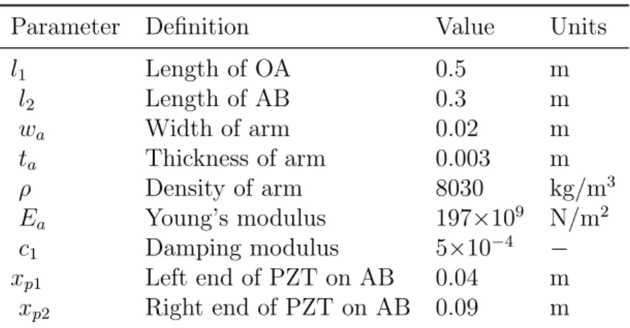
To demonstrate the effectiveness of the proposed design scheme, simulations were conducted by using MATLAB. Parameters of the L-shaped arm and the linear pulse motor are shown in Table 3.1 and Table 3.2, respectively.
Table 3.1: Some parameters of the L-shaped Arm
Parameter Definition Value Units
l1 Length of OA 0.5 m
l2 Length of AB 0.3 m
wa Width of arm 0.02 m
ta Thickness of arm 0.003 m
ρ Density of arm 8030 kg/m3
Ea Young’s modulus 197×109 N/m2 c1 Damping modulus 5×10⁻⁴ −
xp1 Left end of PZT on AB 0.04 m
xp2 Right end of PZT on AB 0.09 m
In the simulation, the sampling interval was 0.01 s, the output y0 was
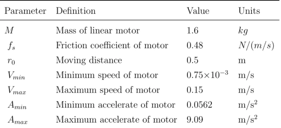
Table 3.2: Parameters of the linear pulse motor
Parameter Definition Value Units
M Mass of linear motor 1.6 kg
fs Friction coefficient of motor 0.48 N/(m/s)
r0 Moving distance 0.5 m
Vmin Minimum speed of motor 0.75×10⁻³ m/s Vmax Maximum speed of motor 0.15 m/s Amin Minimum accelerate of motor 0.0562 m/s2 Amax Maximum accelerate of motor 9.09 m/s2
motor motion control is to reduce the tip displacement of Arm 1 while the motor running as faster as possible with an optimal trajectory.
To be consistent with the experimental conditions, the speed and accel-eration of linear motor were limited within a scope. For the piezoelectric actuator control, the voltage was applied when t > 0 s, output y2 was
con-trolled to track zero.
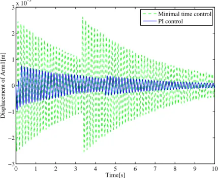
For comparison, firstly we conduct a simulation of the linear motor with minimal time feed-forward control, namely, the motor runs under the maxi-mum speed and acceleration. The vibration of Arm 1 during and after the linear motor motion is shown as the dashed line in Fig. 3.8. As can be seen from the results, the linear motor stops with minimum time consumption at 3.4 s, which leads to biggest arm vibrations, especially at the moment the linear motor starts and stops, which was caused by its biggest accelerations and decelerations, respectively.
0 1 2 3 4 5 6 7 8 9 10 −3
−2 −1 0 1 2 3x 10
−3
Time[s]
Displacement of Arm1[m]
Minimal time control PI control
Figure 3.8: Displacement of Arm 1 with and without feedback control
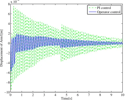
of arm, the motor position and speed is shown in Fig. 3.9. The corresponding vibration of Arm 1 with PI control is compared with the result under minimal time control, as shown in Fig. 3.8, the solid line is displacement under PI control. It illustrates that with PI control, the arm vibration was reduced, but the travel time of the linear motor was longer, arriving at the destination within 4.5 s.
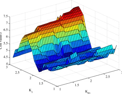
For the optimization problem as shown in Equation (3.12), under a certain weighting factorσ = 1.5×10⁷, and the after stop duration was setted as 0.15
s, with different design parameters, the corresponding cost index J is shown in Fig. 3.10. It illustrates that, by selecting appropriate parameters PI gains
0 1 2 3 4 5 6 7 8 9 10 0
0.2 0.4 0.6 0.8
Time[s]
Motor position[m]
0 1 2 3 4 5 6 7 8 9 10
0 0.05 0.1 0.15 0.2
Time[s]
Motor speed[m/s]
Figure 3.9: Position and speed of motor (with PI control)
minimized, namely, the linear motor motion and arm vibration are balanced.
1 1.5 2 2.5 3 1 1.5 2 2.5 3 4 4.5 5 5.5 6 6.5 7 7.5 K P1 K1 Cost value/J
Figure 3.10: Cost indexes under optimal control with different parameters
be stable.
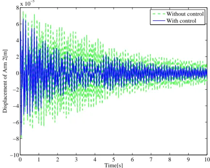
The vibration of Arm 2 without actuator, with actuator no hysteresis compensation and with hysteresis compensation were simulated for compar-ison. Displacement of Arm 2 without the piezoelectric actuator control and with control but without considering hysteresis are shown in Fig. 3.13, the dashed line is vibration of Arm 2 without control, the solid line is vibration of Arm 2 with actuator control, which indicates that the piezoelectric actuator can reduce the arm vibration with the proposed control. The corresponding control input is shown in Fig. 3.14.
Furthermore, by using the hysteresis compensation tracking controllerTC,
0 1 2 3 4 5 6 7 8 9 10 0
0.2 0.4 0.6 0.8
Time[s]
Motor position[m]
0 1 2 3 4 5 6 7 8 9 10
0 0.2 0.4 0.6 0.8 1
Time[s]
Focre input[N]
Figure 3.11: Position speed of motor (with optimal control)
shown in dashed line, the solid line the result using the compensator. The corresponding control input is shown in Fig. 3.16. Fig. 3.15 shows that the proposed controller is effective to further reduce the vibration of arm, which means that both the model of hysteresis and the designed hysteresis compensator are effective.
3.5
Conclusion
0 1 2 3 4 5 6 7 8 9 10 −10
−8 −6 −4 −2 0 2 4 6 8x 10
−4
Time[s]
Displacement of Arm1[m]
PI control Operator control
Figure 3.12: Displacement of Arm 1 with PI motor control and proposed motor control
0 1 2 3 4 5 6 7 8 9 10 −10
−8 −6 −4 −2 0 2 4 6 8x 10
−5
Time[s]
Displacement of Arm 2[m]
Without control With control
Figure 3.13: Displacement of Arm 2 without and with actuator control (with-out hysteresis compensation)
0 1 2 3 4 5 6 7 8 9 10
−50 −40 −30 −20 −10 0 10 20 30 40 50
Time[s]
Control input[v]
0 1 2 3 4 5 6 7 8 9 10 −8
−6 −4 −2 0 2 4 6 8x 10
−5
Time[s]
Displacement of Arm 2[m]
Without compensation With compensation
Figure 3.15: Displacement of Arm 2 without and with hysteresis compensa-tion
0 1 2 3 4 5 6 7 8 9 10
−50 −40 −30 −20 −10 0 10 20 30 40 50
Time[s]
Control input[v]
Operator-based control design
for the L-shaped arm with
unknown load
4.1
Introduction
InSection 4.2, different from last Chapter, the L-shaped arm is modelled as a whole, the load is considered in it. The load estimation method is given based on the model.
In Section 4.3, base on the DWT theory, a short-symmetrical on-line DWT is constructed to use it in the operator-based control design.
In Section 4.4, based on the right coprime factorization method, two operator-based controllers are proposed by using the on-line DWT in it. One controls the motor motion resulting in less arm vibration. Another one further reduces the arm vibration by using a piezoelectric actuator.
In Section 4.5, simulations comparing with previous control are demon-strated to validate performance of the proposed control design.
In Section 4.6, the main contends of this Chapter is summarized.
4.2
Modelling of the system with load
4.2.1
Model of arm vibration with load
In this chapter, the uniform steel L-shaped arm with load is considered, the Motor-Arm structure is shown in Fig. 4.1. The arm is driven by a linear pulse motor to the destination along the motor guide in y direction.
Figure 4.1: System structure
opposite side of AB segment to suppress the arm vibration. The linear motor runs in y direction along the frame, which will result in the arm vibration. Denoting the vibration displacement with time as w(x, t), neglecting the torsional vibration, being seen as an Euler-Bernoulli beam [77], the forced transverse arm vibration is approximated as
EaI ∂4w
∂x4 +csI
∂5y(x, t)
∂x4∂t +ρS
∂2w
∂t2 =q(x, t) (4.1)
where q(x, t) is the external distributed forces on the arm, including the linear motor driving force and the piezoelectric actuator moment. w, stands for w(x, t), is the transverse displacement along the neutral axis of the arm.
cross-Figure 4.2: The sketch of the L-shaped arm
sectional area of the arm, respectively. The arm vibrations at two segments OA and AB can be determined by variables separation method based on the the boundary conditions and the initial conditions of the system, the details about the vibration model arm with load are shown in Appendix A.
We name the OA segment of the arm as Arm 1 and the AB segment as Arm 2, the relative vibration along Arm 1 as y1, and vibration along Arm 2
as y2, they are expressed as follows.
y1(x1, t) =
∞
∑
n=1
J1n(x1)
∫ t
0
[
e−αn(t−τ)sinω
dn(t−τ)f1nu1(τ)]dτ, (4.2)
y2(x2, t) =
∞
∑
n=1
J2n(x2)
∫ t
0
[
e−αn(t−τ)sinω
dn(t−τ)(f2nu2(τ) +f3n)
]
dτ. (4.3)
where, n(n = 1,2,3,· · ·) is the vibration mode order, u1 is the motor force
acted on the arm, u2 = Mp is the moment generated by the piezoelectric
actuator. Jn
1 = Φn1(x1)/ωdn, J2n = Φ2n(x2)/ωdn, αn = c1ωn2 is the damping
factor of the arm vibration. fn
forces, shown as follows.
f1n=−ρS
ms
∫ l1
0
Φn1(x1)dx1,
f2n= ∂Φ
n
2(xp2)
∂x2 −
∂Φn2(xp1)
∂x2
,
f3n=−ρS
ms
∫ l2
0
Φn2(x2)dx2−mtΦn2(l2).
wherems =ma+mt is the total weight of the arm with load,ma is the mass
of the arm. xp1, xp2 are the positions of the both end of the actuator on AB
section as shown in the arm sketch Fig. 4.2.
4.2.2
Load estimation method
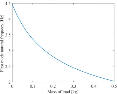
As shown in the Appendix A, the mass of the load will impact the arm vibration dynamics, especially the important parameters in the vibration model, such as the natural frequency of every mode, the frequency decreases with the increasing of the load mass. According to Eq. (A.24), it obtains that
βn=
4
√
ρS(2πfn)2 EaI
(4.4)
From the Eq. (A.21) shown in Appendix A, it yields
mt= PI PII
ρS
β (4.5)
where
PI = sinβl−sinhβl+−sinhβl−sinβl+−2 cosβl2coshβl2−2 cosβl1coshβl1
−2 cosβl+coshβl+−2
PII = 2 cosβl+sinhβl+−2 coshβl+sinβl++ 2 cosβl2sinhβl2−coshβl2sinβl2
According to Eq. (4.5), the relationship between the first mode frequency and load mass is shown in Fig. 4.3.
0 0.1 0.2 0.3 0.4 0.5
Mass of load [kg] 2
2.5 3 3.5 4 4.5
First mode natural frequecy [Hz]
Figure 4.3: The relationship between the first mode frequency and load mass
If we can measure the natural frequency of one mode of the arm vibration in experiment, such as f1 (Hz), according to the relationship in Eq. (4.4),β1
is obtained, substitute it into the frequency equation (4.5), the mass of load could be estimated.
The load mass estimation flow is given as: initial vibration → y1(t) →
4.3
On-line wavelet transform
The DWT decomposes a time domain signal into an orthogonal set of wavelets, presented in time-frequency domain, which is useful for different purposes. However, most DWT applications are off-line needing the entire signal. These approaches are not suitable for the real-time vibration control. To solve the problem and apply wavelet transforms to arm vibration controls, a real-time wavelet approach is implemented in this section.
The on-line DWT usually utilizes a moving window . When the control loop starts, the on-line DWT must wait for the available signal with length equal to ln. The lager the ln, the more significant time delay. On the other
hand, with smallerln, the DWT results in lower accuracy. In this dissertation,
the size of the moving windowln depends on the sampling frequency and the
vibration frequency band considered in the controller. For a certain fs, the
considered frequency band decides the wavelet decomposition levels L, then the size of the moving window ln is decided.
To deal with the boundary effects, one of the methods is artificially extend the signals at boundaries before processing. Symmetric extension is usually adopted to keep the continuity. However, the whole symmetrization will increase the computation load, probably causes time delay for the control and lower the performance. Therefore, we extend the data stream using short-symmetrical, the length of extension is denoted aslt,lw =ln+lt, lw is
and ˆy are defined as follows.
Wi =
{
none, i < ln
y(i−ln+ 1),· · · , y(i), y(extension), i≥ln
(4.6)
y(extension) = [y(i),· · · , y(i−lt+ 1)]
ˆ
y(i) =
{
y(i), i < ln ywti(ln), i≥ln
(4.7)
where ywti = DW T(Wi) is the output of the on-line DWT for the moving
window Wi. The on-line DWT process is shown in Fig. 4.4.
4.4
Operator-based control design with DWT
For some nonlinear systems, the disturbances are complicated and unknown. It is difficult to satisfy the factorization conditions and robustness condition as shown in (2.19). In addition, if the disturbances include high frequency signal, the system output will fluctuate severely; the performances of the system will degrade. Therefore, we use an on-line DWT in the operator-based control, the control scheme is shown in Fig. 4.5. A DWT processor is added between the system outputyaand operatorAto decompose the output yainto time-frequency domain. According to the characteristics of the system
dynamic, the necessary signal components are extracted and reconstructed as ˆy. If the unwanted disturbances are fully removed, namely ˆy ≃ y, the coprime condition (2.18) approximates the condition (2.15), then the desired operatorsA and B could be obtained more easily.
Figure 4.5: Nonlinear operator-based robust control with DWT

![Figure 3.15: Displacement of Arm 2 without and with hysteresis compensa- compensa-tion 0 1 2 3 4 5 6 7 8 9 10−50−40−30−20−1001020304050 Time[s]Control input[v]](https://thumb-ap.123doks.com/thumbv2/123deta/6857954.243250/71.918.245.680.232.590/figure-displacement-hysteresis-compensa-compensa-time-control-input.webp)