MEASURING OVERALL HEALTH SYSTEM PERFORMANCE FOR 191 COUNTRIES
Ajay Tandon, Christopher JL Murray
Jeremy A Lauer David B Evans
GPE Discussion Paper Series: No. 30 EIP/GPE/EQC
World Health Organization
1. Introduction
Performance of health systems has been a major concern of policy makers for many years. Many countries have recently introduced reforms in the health sector with the explicit aim of improving performance (1,2). There exists an extensive literature on health sector reform, and recent debates have emerged on how best to measure performance so that the impact of reforms can be assessed (3). Measurement of performance requires an explicit framework defining the goals of a health system against which outcomes can be judged and performance quantified (4).
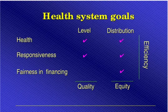
In a previous paper, Evans et al. (5) describe how the performance of countries in terms of meeting one important goal – that of maximising population health – can be measured. In this companion paper, we assess the performance of countries in terms of achieving a broader set of health system outcomes. In addition to considering health, we include attainment in terms of 4 other indicators linked to the intrinsic goals of a health system. The analytical framework used for characterising the goals of a health system is derived from Murray and Frenk (6). They differentiate intrinsic goals of the health system from instrumental goals. In their framework, an intrinsic goal is one: (a) whose attainment can be raised while holding other intrinsic goals constant (i.e., there is at least partial independence among the different intrinsic goals), and (b) raising the attainment of which is in itself desirable, irrespective of any other considerations. Instrumental goals, on the other hand, are goals that are pursued to attain the instrinsic goals. Murray and Frenk identify three intrinsic goals of a health system (Figure 1).
Health system goals
Health system goals
Health
Health
Responsiveness
Responsiveness
Fairness in financing
Fairness in financing
Level
Level Distribution Distribution
✔
✔
✔
✔
✔
✔
✔
✔
✔
✔
Effic ienc y Effic ienc y
Quality
Quality Equity Equity
Figure 1: Health System Goals
The first is improvement in the health of the population (both in terms of levels attained and distribution). The second is enhanced responsiveness of the health system to the legitimate expectations of the population. Responsiveness in this context explicitly refers
to the non-health improving dimensions of the interactions of the populace with the health system, and reflects respect of persons and client orientation in the delivery of health services, among other factors.1 As with health outcomes, both the level of responsiveness and its distribution are important. The third intrinsic goal is fairness in financing and financial risk protection. The aim is to ensure that poor households should not pay a higher share of their discretionary expenditure on health than richer households, and all households should be protected against catastrophic financial losses related to ill health.2
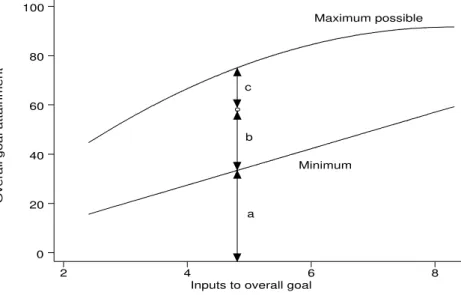
Methodologically, overall health system performance in relation to this broader set of goals is assessed in a similar fashion as described in Evans et al. (5). Specifically, overall performance measures how well a country achieves all five goals of the health system simultaneously, relative to the maximum it could be expected to achieve given its level of resources and non-health system determinants. Adjustment is also made for the fact that overall goal attainment may not be zero in the absence of a modern health system. The framework of frontier production functions (a concept typically used in the measurement of the technical efficiency of firms and farms) is applied, in which the health system as a whole is viewed as a macro-level production unit. The concept is illustrated in Figure 2. The vertical axis measures overall goal attainment and inputs are measured on the horizontal axis.
Inputs to overall goal
2 4 6 8
0 20 40 60 80 100
a b c
Maximum possible
Minimum
Overall goal attainment
Figure 2: Health System Performance (Overall Efficiency)
The upper line represents the frontier, or the maximum possible level of attainment that can be achieved for given levels of inputs. The lower line, labelled “minimum”, represents the minimum level of attainment that would exist even in the absence of any health system inputs (e.g., the entire population will not be dead in the absence of a functioning health system). Assume a country is observed to achieve (a+b) units of the overall goal attainment. Murray and Frenk define overall system performance as b/(b+c). This indicates what a system is achieving relative to its potential at given input levels.
1 Health-improving responsiveness dimensions of the system would be included in the attainment of the goal of improving population health. See de Silva et al. (18) for additional details.
2 See Murray et al. (19) for details.
The idea is very similar to that of technical efficiency in the frontier production function literature.3 Accordingly, we use the term “overall efficiency” to refer to overall health system performance in the remainder of this paper.
2. Estimation Methods a) Composite Index
In order to assess overall efficiency, the first step was to combine the individual attainments on all five goals of the health system into a single number, which we call the composite index. The composite index is a weighted average of the five component goals specified above. First, country attainment on all five indicators (i.e., health, health inequality, responsiveness-level, responsiveness-distribution, and fair-financing) were rescaled restricting them to the [0,1] interval. Then the following weights were used to construct the overall composite measure: 25% for health (DALE), 25% for health inequality, 12.5% for the level of responsiveness, 12.5% for the distribution of responsiveness, and 25% for fairness in financing. These weights are based on a survey carried out by WHO to elicit stated preferences of individuals in their relative valuations of the goals of the health system.4
The idea of using a weighted average as an index of several goals is not new. A recent example is the Human Development Index (HDI), an index based on the average of three indicators: longevity, educational attainment (including literacy and enrolment), and income per capita. (7). The HDI is commonly used to assess the state of development of a country. Factors such as health and educational levels of the populace are not viewed as instrumental goals aimed at achieving higher productivity and thereby higher income levels, but are viewed as intrinsic goals of development.5 A similar idea underlies the construction of the composite index as a measure of the overall attainment of the intrinsic goals of the health system.
Figure 3 reports the rank correlation between attainment on each of the individual components and attainment on the overall composite index for the 191 countries which are members of the World Health Organization (WHO) in 1997.
3 Technical efficiency is typically defined as (a+b)/(a+b+c) in Figure 2. The primary difference between performance and technical efficiency is that the former accounts for the non-zero outcome even in the absence of inputs.
4 See Gakidou et al. (20) for details of the survey.
5 For an extension of the HDI that incorporates inequalities in income, education, and health, see Hicks (21).
Responsiveness Level
1 191
1 191
1 191
1 191
Responsiveness
Fair Finance
1 191
Health Inequality
DALE
1 191
COMPOSITE Distribution
Figure 3: Rank Correlation, Individual Goal Attainment versus Composite Attainment
As can be seen from the bottom row of Figure 3, the ranks on DALE and health inequality are the most highly correlated with the overall composite, with countries which are ranked high on these two components also ranking high on the composite index. This is likely a product of the relatively high rank correlation between some of the goals, e.g., countries which rank high on levels of health also seem to do well on level of responsiveness. Rankings on responsiveness level are also highly correlated with responsiveness distribution, as are rankings on health level with health distribution. Rankings on fair financing do not seem to be correlated with ranks on any of the other components. This implies that countries which have major inequalities in health or responsiveness are equally as likely to score well on fair financing as countries which have less inequality in these variables. And countries which achieve relatively high levels of health are no less likely to have unfair financial systems as countries that achieve relatively low health outcomes.
For the purposes of this analysis, the weights used in the construction of the composite index have been used consistently, i.e., without considering uncertainty in the valuations of the different components. See Murray et al. (8) for additional details regarding the weighting scheme and a sensitivity analysis of the impact of changes in these weights on the overall attainment of the health system as measured by the composite index.
b) Methodology
The econometric methodology for measuring efficiency on the composite index (i.e., overall efficiency) is identical to that for measuring efficiency on health [See Evans et al. (5) for more details]. The problem, from an econometric standpoint, is the estimation of the maximum attainable composite index (the frontier) given resource inputs and other non health-system determinants of goal attainment. Since this frontier is not directly observable, one way to identify it is to estimate it from the data. There is a large literature on this topic, especially in the areas of agricultural and industrial economics. For reasons elaborated in Evans et al. (5), we chose to use a fixed-effects panel data model in the
estimation of the frontier. The econometric methodology of the fixed-effects model is elaborated below. Estimation of the minimum level of goal attainment in the absence of a health system is described later.
Consider a functional relationship where the simultaneous attainment of the goals of the health systems are a function of resource inputs and other non-health system determinants. In equation form, this can be written as:
i it it
it X v u
Y =α + ′β + − . (i)
The dependent variable Yit is the composite index of country i in time t, and X´ is a vector of independent variables. vit is the error term representing random noise with mean zero. The term ui A 0 measures country-specific technical inefficiency. It is constrained to be always non-negative. The above model can be rewritten as:
it it i
it X v
Y =α + ′β + , (ii)
where the new intercept αi = (α - ui) is now country-specific, and estimates can be found by using a standard fixed-effects model. α represents the frontier intercept, and the ui’s represent country-specific inefficiencies. In order to ensure that all the estimated ui’s are positive, the country with the maximum αi is assumed to be the reference and is deemed fully efficient. Mathematically,
) ˆ max(
ˆ αi
α = , (iii)
and
i
uˆi=αˆ−αˆ. (iv)
This normalisation ensures non-negative ui’s. Technical efficiency is defined as:
) , 0
| (
) ,
| (
it i
it
it i it i
X u Y E
X u Y TE E
= = . (v)
Overall efficiency (Ei) was based on this definition of technical efficiency with the difference that the minimum output (Mit) that would be achieved in the absence of a health system was subtracted.
) . , 0
| (
) ,
| (
it it i
it
it it i it i
M X u Y E
M X u Y E E
−
=
= − (vi)
In less technical terms:
.
min max
min i i
i i
i
COMPOSITE COMPOSITE
COMPOSITE COMPOSITE
E −
= − (vii)
Where the COMPOSITE index in the above equation refers to the expected value for country i estimated from the model.
c) Model Specification
Different functional formulations of the fixed-effect model were estimated. Modern production studies generally use a flexible form. One of the most versatile is the translog (or the transcendental logarithmic) model. For the two-input case (X1, X2), the translog model can be written as follows (all variables in logs):
it it it it
it it
it i
it X X X X X X v
Y =α +β1 1 +β2 2 +β3( 1 )2 +β4( 2 )2 +β5( 1 )( 2 )+ . In effect, the translog function is a second-order Taylor-series approximation to an unknown functional form (9,10). Both the Cobb-Douglas and the Constant Elasticity of Substitution (CES) production functions can be derived as restricted formulations of the translog function (11). We estimated the full translog model as well as nested versions of the model including the Cobb-Douglas log-linear formulation, and the Cobb-Douglas log-linear with each of the square terms and the interaction term separately.
d) Data
To measure efficiency using the production function approach, data on three general types of variable are necessary. First, it is necessary to identify an appropriate outcome indicator that represents the output of the health system. Second, it is necessary to measure the health-system inputs that contribute to producing that output, and third, it is necessary to include the effect of controllable non-health-system determinants of health. The composite index was considered to be the output of the health system. Details of its construction have been described earlier. Inputs considered included total health expenditure per capita (public and private) in 1997 international dollars (using purchasing power parities, or PPPs, to convert from local currency units). The data sources and methods of calculation of health expenditure are described elsewhere (12,13). As a proxy for non-health systems inputs, we considered educational attainment (as measured by average years of schooling in the population older than 15 years). Our panel covers the years from 1993 to 1997 for all 191 member countries of WHO, with some missing data for some countries and years. While every country had an observation for 1997, about 50 countries had observations only for that year (i.e., the remaining 141 countries were complete in all panel years).
It is important to note that, by using health expenditure as the health system input to the production of health outcomes, the interpretation of overall efficiency differs significantly to the interpretation of efficiency from many existing production function studies. There, efficiency relates only to technical efficiency – whether the observed combination of inputs produces the maximum possible output. But overall efficiency in our specification is not just a function of technical efficiency. It will also vary according to the choices each country makes about the mix of interventions purchased with the available health expenditures. Accordingly, overall efficiency combines both technical and allocative efficiency.
e) Minimum Frontier
What level of composite index could be expected in the absence of a health system? This is analogous to the question posed in Evans et al. (5). In that paper, the goal was to estimate the minimum level of health, measured in terms of disability adjusted life expectancy or DALEs, that would be expected even in the absence of a modern health system.6 In the case of the composite index, however, two components of the overall attainment measure (i.e., “fair financing” and “responsiveness-distribution”) have little or no meaning in the absence of a health system. In other words, everyone in the population is equally well (or poorly) off with respect to a non-existent system of health financing, and if there is no responsiveness to distribute, a similar argument can be made for responsiveness-distribution. For this reason, these two components of the composite index are given full scores in determination of the minimum (in calculating the weighted average this would entail that attainment of these goals be given a score of 37.5, i.e., 25×1+12.5×1 = 37.5).
For similar reasons, it is assumed that the score for the other two components (“health inequalities” and “responsiveness-level”) would be zero in the absence of a health system (25×0+12.5×0 = 0). Since a non-existent health system is clearly completely unresponsive, responsiveness-level receives a zero score. However, although health inequalities surely would exist in the absence of a health system, with respect to the health system goal of reducing inequalities, zero progress can be claimed.
Furthermore, since each component of the composite index is normalised on the [0,1] interval, the component accounting for health level (DALE) is similarly normalised for calculation for the minimum attainable bound. Thus, the equation for the bottom frontier is as follows (where 25 is the weight on health level in the overall attainment measure):
( )
ùêë é
−
× − +
=
min max
min 37.5 25 min
DALE DALE
DALE
COMPOSITEi DALEi (8)
The value of DALEmin and DALEmax were set at 20 and 80, respectively. So long as the observed DALE values in the sample are restricted to [0,1] after normalisation, and so long as the same bounds are used in calculating the composite score and in calculating the minimum, the choice of the normalisation has no intrinsic importance.7
In order to obtain an expression for DALEmin, a sub-sample of the cross-section of 25 countries for which data was compiled at around the turn of the century was investigated, and the minimum frontier production function for health as a function of literacy was obtained [see Evans et al. (12) and Evans et al. (5) for more details]. This linear relation was similarly used to predict, at current levels of literacy, the health levels that would be achieved in the absence of a health system.
f) Uncertainty
6 Unlike a traditional production setting, some amount of health or other health-system goal attainment is to be expected despite no resource inputs to the health sector.
7 Note, for example, that in Evans et al. (5), minimum DALE was always A 15.
Uncertainty in the COMPOSITE index reflects the underlying uncertainty in the estimation of each of the five goals of the health systems for all 191 countries. Given that we had a 1000 random draws on the values of each of the five goals of the health system for each country, we were able to construct a distribution consisting of 1000 draws on the composite index for each country. In order to derive the confidence intervals around our statistic of interest, the overall efficiency measure, Monte Carlo simulation techniques were used. In brief, the efficiency index was estimated using the fixed-effect model for all countries 1000 different times, where each of the 1000 estimates reflected a single draw from the distribution of the composite index. The 80% uncertainty intervals on the overall efficiency index reflect the estimated distribution of the efficiency index derived from these 1000 different regressions.8 Rank order was based on the mean value of the overall efficiency index for each country, where the 80% uncertainty intervals for the rank order were derived from the distribution of the overall efficiency index.
3. Results
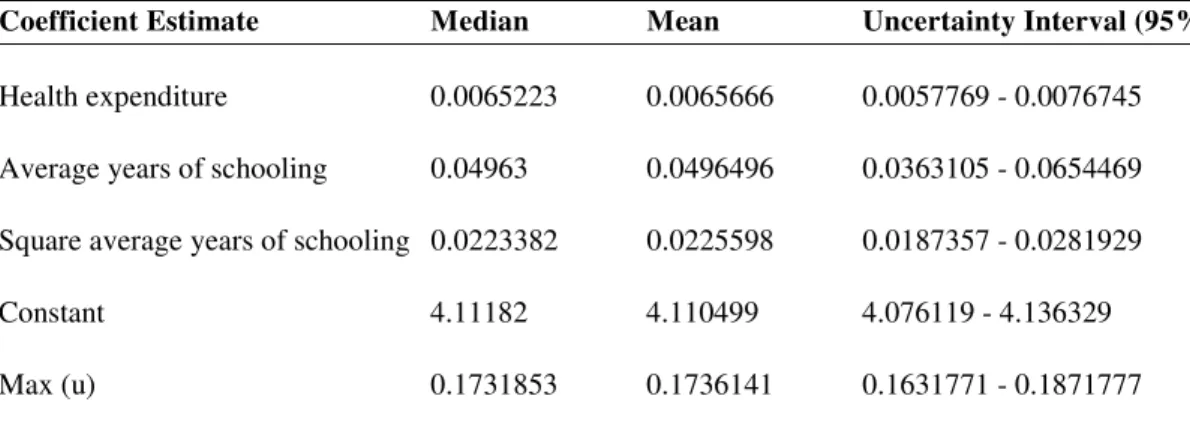
Results from the preferred functional form estimated using the fixed effect model are reported in Table 1.
Table 1. Coefficient Estimates (Median, Mean and Uncertainty Interval) for the Frontier Health Production Function, Logged Variables, 191 Member Countries of WHO, Panel Estimates (1993– 1997).
Coefficient Estimate Median Mean Uncertainty Interval (95%)
Health expenditure 0.0065223 0.0065666 0.0057769 - 0.0076745 Average years of schooling 0.04963 0.0496496 0.0363105 - 0.0654469 Square average years of schooling 0.0223382 0.0225598 0.0187357 - 0.0281929
Constant 4.11182 4.110499 4.076119 - 4.136329
Max (u) 0.1731853 0.1736141 0.1631771 - 0.1871777
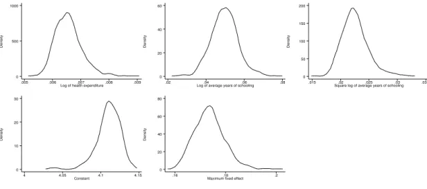
The table also shows the 95% uncertainty intervals around the estimated coefficients. These uncertainty intervals are not the statistical confidence intervals of the individual regressions. They were derived by omitting the lowest and the highest 2.5% of the coefficient estimates from the 1000 regressions described earlier. Here, 95% uncertainty intervals were used because they offer greater discriminatory power against the null hypothesis that the coefficients are equal to zero. None of the uncertainty intervals include zero. The simulated distributions of the individual coefficients are graphed in Figure 5. The constant term represents the average fixed effect in the sample. Max(u) is the maximum deviation from this average and, when added to the constant, gives the intercept for the frontier.
8 See Evans et al. (5) for details.
Density
Log of health expenditure
.005 .006 .007 .008 .009
0 500 1000
Density
Log of average years of schooling
.02 .04 .06 .08
0 20 40 60
Density
Square log of average years of schooling
.015 .02 .025 .03 .035
0 50 100 150 200
Density
Constant
4 4.05 4.1 4.15
0 10 20 30
Density
Maximum fixed effect
.16 .18 .2
0 20 40 60 80
Figure 5: Distribution of the Coefficient Estimates for Log of Health Expenditure, Log of Average Years of Schooling, Square of Log of Average Years of Schooling, Constant, and Maximum Value of the Country-Specific Fixed Effect
We also tested statistically whether we should use a fixed effects or random effects model. The Hausman test is a test of equality between the coefficients estimated via the fixed-effects and random-effects models. Assuming that the model is correctly specified, a significant difference in the coefficient estimates is indicative of correlation between the individual effects and the regressors. Where this correlation is present, the estimates using a random-effects model will be biased (14,15). Table 2 reports the coefficient estimates where the expected value of the composite index is used as the dependent variable. As can be seen from the test statistic, the null of no correlation is rejected and a fixed-effects model is clearly preferable.
Table 2. Hausman Specification Test: Coefficient Estimates using Expected Value of the Composite Index as Dependent Variable. All Variables in Logs, 191 WHO Member Countries, Panel Estimates (1993-1997).
Coefficients
Composite index Fixed-Effects Random-Effects Difference
Health expenditure 0.0065425 0.0119787 -0.0054362
Average years of schooling 0.0494743 0.0546144 -0.0051401
Square of average years of schooling 0.0227706 0.0379717 -0.0152011
m2(3) 59.02
p value 0.000
The resulting estimates of overall efficiency (i.e., performance) for each country are reported in Annex Table 1, along with the uncertainty interval around the efficiency
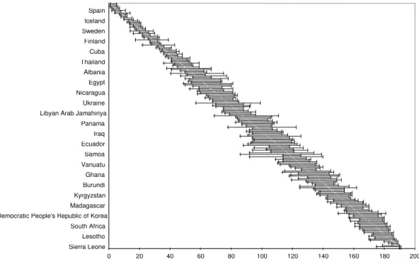
index. The efficiency index ranges from a maximum of 0.994 for France and a minimum of 0 for Sierra Leone. In any given regression, the country with the maximum fixed effect will have a score of 1. However, the reported scores are averaged over 1000 runs, and France was not the best-performing country in all 1000 runs. Furthermore, there is substantial overlap of the confidence intervals for several countries. It would not be possible to say, for instance, that the rank orders of the top three countries (France, Italy, and San Marino) with respect to the overall efficiency were significantly different from each other. This overlap in the rankings is illustrated graphically in Figure 6.
0 20 40 60 80 100 120 140 160 180 200
Sierra Leone Lesotho South Africa Democratic People's Republic of Korea Madagascar Kyrgyzstan Burundi Ghana Vanuatu Samoa Ecuador Iraq Panama Libyan Arab Jamahiriya Ukraine Nicaragua Egypt Albania Thailand Cuba Finland Sweden Iceland Spain
Figure 6: Uncertainty Intervals, Ranking of Overall Efficiency, 191 countries
According to the interpretation of the translog model as a second-order approximation to an unknown functional form, the full version of the translog is, a priori, the reference standard. However, when parsimony is added as a criterion for model choice, the model we report – with log of health expenditure, log of average years of schooling and the square of average years of schooling as regressors – is both parsimonious and maps most closely to the reference standard (Figure 7). We compare rank order correlation in Figure 7 since efficiency will invariably increase with the addition of terms on the right hand side of the regression (unless the added term is completely collinear with another, it will always explain additional sample variance). Thus, the appropriate criterion for judging predictive stability across models is rank order correlation.
Health expenditure
1 191
1 191
1 191
1 191
Years of schooling
Square of health expenditure
1 191
Interaction
1 191
Health expenditure Health expenditure
Health expenditure Health expenditure
Health expenditure Years of schooling
Years of schooling
Years of schooling
Years of schooling Square of years of schooling
Square of health expenditure Square of years of schooling
Square of health expenditu
Interaction Years of schooling
Square of years of schoolin
Figure 7: Rank Correlation Matrix for Different Model Specifications
The above results (Figure 7) show clearly that the rank of the different countries is very robust to the functional form of the translog regression. The rank correlations are extremely high no matter what combination of variables is included, suggesting that poor performers perform poorly in all specifications and rank is not an artefact of the choice of model. Conversely, high performers perform well in all specifications.
To further test robustness, we explored whether the inclusion of possible other non-health system determinants of health would make a difference to the ranking – in addition to our proxy for non-health system determinants, average years of schooling. Since other possible direct explanators were difficult to identify and measure for all countries in our sample, we defined a new variable obtained by regressing income per capita on the regressors already in our efficiency equation. The residual from the regression of income on health expenditure per capita, average years of schooling, and average years of schooling squared was estimated. This residual can be interpreted as the part of income which might act through mechanisms other than health expenditures and education – or possible other pathways (called POSOTHER). POSOTHER was added to the fixed effects regression as a proxy for these possible other pathways related to income, and the efficiency analysis and ranks were recomputed.
When any new explanator is added to an equation, the residual of the dependent variable that is left unexplained is smaller, and accordingly the efficiency index is higher with POSOTHER. However, the correlation between the rankings under the two sets of estimates is very high (0.9974) showing that inclusion of POSOTHER does not have a significant impact on the relative rankings of the countries based on their efficiency in producing health. For this reason, and because it is not possible to explain which determinants of efficiency picked up by POSOTHER are controllable inputs or not, we chose to use the more parsimonious form of the equation reported above.
4. Discussion
This paper has introduced a new way of measuring the efficiency of health systems. Unlike previous work in this area, we have specifically defined the broad set of goals of the health system such as responsiveness (both level and distribution), fair financing, and health inequality, in addition to the more traditional goal of population health. By way of comparison, Figures 8 and 9 report the estimates of efficiency on health as well as overall efficiency (with uncertainty intervals) against health expenditure per capita (in log).9
Efficiency on health
Log of health expenditure per capita
2 4 6 8
0 .5 1
Figure 8: Health Efficiency versus Health Expenditure per Capita
9 Efficiency on health is from Evans et al. (5).
Overall efficiency
Log of health expenditure per capita
2 4 6 8
0 .5 1
Figure 9: Overall Efficiency versus Health Expenditure per Capita
Several things are notable: first, there is greater uncertainty related with the estimates of overall efficiency compared to efficiency on health, which reflects the fact that there are uncertainty intervals around each of the components of the composite index. Secondly, efficiency on health appears to increase with health expenditure per capita and then perhaps to decline slightly. This is also the case for overall efficiency, but there the decline is less obvious. One interpretation of this could be that there are diminishing returns to increasing the inputs of resources devoted to producing health (say due to biological limits on life expectancy), but that the composite index would not be subject to strong diminishing returns because greater expenditure can be used to further the goals of responsiveness, fair financing, and reductions in health inequality.
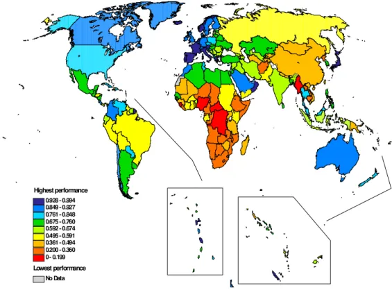
This association of overall efficiency with resource inputs is also evident from the country rankings: industrialised countries are dominant among the better performers. Most of those countries that are ranked low tend to be those in Sub-Saharan Africa where a combination of factors related to economic problems, civil unrest, and high AIDS prevalence is likely to have a deleterious effect on overall efficiency. Figure 10 plots the geographical distribution of the overall efficiency score.
0.928 - 0.994 0.849 - 0.927 0.761 - 0.848 0.675 - 0.760 0.592 - 0.674 0.495 - 0.591 0.361 - 0.494 0.200 - 0.360 0 - 0.199
No Data
The boundaries and names shown and the designations used on this map do not imply the expression of any opinion whatsoever on the part of the World Health Organization concerning the legal status of any country, territory, city or area or of its authorities, or concerning the delimitation of its frontiers or boundaries. Dotted lines on maps represent approximate border lines for which there may not yet be full agreement. WHO 2000. All rights reserved
Highest performance
Lowest performance
Figure 10: Global Distribution of Overall Efficiency, 191 WHO Member States, 1997 Estimates
Higher overall goal attainment can be achieved by increasing health expenditure. This implies moving along the expansion path in the spirit of the World Health Report 1999 (16). This is illustrated in Figure 11, which plots predicted levels of overall goal attainment as a function of health expenditure and educational attainment for our preferred frontier equation.
100
health expenditure 1000
2 5
10
average years of schooling 75
85 95 composite index
100
health expenditure 1000
Figure 11: Logarithmic-Scale Plot of the Expected Value of the Overall Health System Achievement Frontier Production Function, 191 Member Countries of WHO, Panel Estimates (1993–1997)
However, the analysis also suggests that overall goal attainment can be increased without increasing health expenditure: there is considerable room in all countries, at all levels of health expenditure, to increase efficiency as well. This raises the question of how to increase efficiency, something that is discussed further in the World Health Report 2000 (17).
This work draws attention to the fact that some countries are doing better than others in terms of achieving their potential, given their inputs. Future work will aim to identify determinants of this relative performance: whether exogenous factors such as institutional quality and population density have an impact on efficiency. It is also important to note that the analysis does not imply that countries with high efficiency scores cannot improve their performance. There is an implicit overestimation of efficiency in the model since the estimates assume that the best-performing country in the sample has an efficiency of 1, or is perfectly efficient. This is unlikely to be the case, but at present we have no way of knowing the extent of the overestimation.
Since it is not restricted by possible biological limits on healthy life-span, overall efficiency is a more representative measure of the true efficiency of health systems than one based on health status alone. It is an indicator that is feasible to measure regularly enabling comparison between countries, and over time within the same country. The framework for measuring overall efficiency may also be applied at a sub-national level, say to conduct a comparison of health systems at the district or state level. This is the focus of ongoing work at WHO. Such intra-national and inter-temporal analyses of efficiency would be particularly important for countries introducing health system reforms, and we hope that this study encourages all countries to routinely measure the inputs and outputs of their health systems. An important benefit from the debate that is likely to accompany this exercise will be development of improved data sources and estimation methods. In taking this first step towards measuring efficiency, the goal is to stimulate action that will eventually improve the overall performance of health systems in countries and contribute to improving the welfare of people.
ANNEX
Table 1. Overall efficiency in all WHO member states
Overall efficiency
Rank Uncertainty Interval
Member State Index Uncertainty Interval
1 1 - 5 France 0.994 0.982 - 1.000
2 1 - 5 Italy 0.991 0.978 - 1.000
3 1 - 6 San Marino 0.988 0.973 - 1.000
4 2 - 7 Andorra 0.982 0.966 - 0.997
5 3 - 7 Malta 0.978 0.965 - 0.993
6 2 - 11 Singapore 0.973 0.947 - 0.998
7 4 - 8 Spain 0.972 0.959 - 0.985
8 4 - 14 Oman 0.961 0.938 - 0.985
9 7 - 12 Austria 0.959 0.946 - 0.972
10 8 - 11 Japan 0.957 0.948 - 0.965
11 8 - 12 Norway 0.955 0.947 - 0.964
12 10 - 15 Portugal 0.945 0.931 - 0.958
13 10 - 16 Monaco 0.943 0.929 - 0.957
14 13 - 19 Greece 0.933 0.921 - 0.945
15 12 - 20 Iceland 0.932 0.917 - 0.948
16 14 - 21 Luxembourg 0.928 0.914 - 0.942
17 14 - 21 Netherlands 0.928 0.914 - 0.942
18 16 - 21 United Kingdom 0.925 0.913 - 0.937
19 14 - 22 Ireland 0.924 0.909 - 0.939
20 17 - 24 Switzerland 0.916 0.903 - 0.930
21 18 - 24 Belgium 0.915 0.903 - 0.926
22 14 - 29 Colombia 0.910 0.881 - 0.939
23 20 - 26 Sweden 0.908 0.893 - 0.921
24 16 - 30 Cyprus 0.906 0.879 - 0.932
25 22 - 27 Germany 0.902 0.890 - 0.914
26 22 - 32 Saudi Arabia 0.894 0.872 - 0.916
27 23 - 33 United Arab Emirates 0.886 0.861 - 0.911
28 26 - 32 Israel 0.884 0.870 - 0.897
29 18 - 39 Morocco 0.882 0.834 - 0.925
30 27 - 32 Canada 0.881 0.868 - 0.894
31 27 - 33 Finland 0.881 0.866 - 0.895
32 28 - 34 Australia 0.876 0.861 - 0.891
33 22 - 43 Chile 0.870 0.816 - 0.918
34 32 - 36 Denmark 0.862 0.848 - 0.874
35 31 - 41 Dominica 0.854 0.824 - 0.883
36 33 - 40 Costa Rica 0.849 0.825 - 0.871
37 35 - 44 United States of America 0.838 0.817 - 0.859
38 34 - 46 Slovenia 0.838 0.813 - 0.859
39 36 - 44 Cuba 0.834 0.816 - 0.852
40 36 - 48 Brunei Darussalam 0.829 0.808 - 0.849
41 38 - 45 New Zealand 0.827 0.815 - 0.840
42 37 - 48 Bahrain 0.824 0.804 - 0.845
43 39 - 53 Croatia 0.812 0.782 - 0.837
44 41 - 51 Qatar 0.812 0.793 - 0.831
45 41 - 52 Kuwait 0.810 0.790 - 0.830
46 41 - 53 Barbados 0.808 0.779 - 0.834
47 36 - 59 Thailand 0.807 0.759 - 0.852
48 43 - 54 Czech Republic 0.805 0.781 - 0.825
49 42 - 55 Malaysia 0.802 0.772 - 0.830
50 45 - 59 Poland 0.793 0.762 - 0.819
51 38 - 67 Dominican Republic 0.789 0.735 - 0.845
52 41 - 67 Tunisia 0.785 0.741 - 0.832
53 47 - 62 Jamaica 0.782 0.754 - 0.809
54 50 - 64 Venezuela, Bolivarian 0.775 0.745 - 0.803
Republic of
55 41 - 75 Albania 0.774 0.709 - 0.834
56 51 - 63 Seychelles 0.773 0.747 - 0.797
57 47 - 77 Paraguay 0.761 0.714 - 0.806
58 55 - 67 Republic of Korea 0.759 0.740 - 0.776
59 50 - 78 Senegal 0.756 0.711 - 0.800
60 53 - 73 Philippines 0.755 0.720 - 0.789
61 52 - 74 Mexico 0.755 0.719 - 0.789
62 54 - 73 Slovakia 0.754 0.721 - 0.781
63 49 - 81 Egypt 0.752 0.707 - 0.798
64 50 - 80 Kazakhstan 0.752 0.699 - 0.802
65 55 - 80 Uruguay 0.745 0.702 - 0.782
66 59 - 74 Hungary 0.743 0.713 - 0.768
67 53 - 81 Trinidad and Tobago 0.742 0.695 - 0.784
68 59 - 75 Saint Lucia 0.740 0.717 - 0.765
69 58 - 81 Belize 0.736 0.697 - 0.772
70 60 - 81 Turkey 0.734 0.698 - 0.764
71 58 - 83 Nicaragua 0.733 0.696 - 0.770
72 64 - 84 Belarus 0.723 0.691 - 0.750
73 65 - 82 Lithuania 0.722 0.690 - 0.750
74 63 - 83 Saint Vincent and the Grenadines
0.722 0.686 - 0.754
75 66 - 81 Argentina 0.722 0.695 - 0.747
76 68 - 84 Sri Lanka 0.716 0.692 - 0.740
77 68 - 85 Estonia 0.714 0.684 - 0.741
78 57 - 99 Guatemala 0.713 0.642 - 0.774
79 70 - 88 Ukraine 0.708 0.674 - 0.734
80 68 - 93 Solomon Islands 0.705 0.664 - 0.739
81 70 - 92 Algeria 0.701 0.669 - 0.730
82 75 - 88 Palau 0.700 0.679 - 0.719
83 75 - 88 Jordan 0.698 0.675 - 0.720
84 75 - 91 Mauritius 0.691 0.665 - 0.719
85 74 - 96 Grenada 0.689 0.652 - 0.723
86 76 - 93 Antigua and Barbuda 0.688 0.657 - 0.718 87 79 - 96 Libyan Arab Jamahiriya 0.683 0.655 - 0.707
88 69 - 111 Bangladesh 0.675 0.618 - 0.732
89 83 - 107 The former Yugoslav Republic of Macedonia
0.664 0.630 - 0.695 90 84 - 106 Bosnia and Herzegovina 0.664 0.632 - 0.694
91 85 - 104 Lebanon 0.664 0.638 - 0.688
92 85 - 107 Indonesia 0.660 0.632 - 0.689
93 83 - 110 Iran, Islamic Republic of 0.659 0.620 - 0.693
94 87 - 108 Bahamas 0.657 0.625 - 0.687
95 87 - 107 Panama 0.656 0.627 - 0.686
96 90 - 106 Fiji 0.653 0.630 - 0.674
97 78 - 123 Benin 0.647 0.573 - 0.710
98 94 - 107 Nauru 0.647 0.630 - 0.664
99 92 - 110 Romania 0.645 0.624 - 0.666
100 90 - 113 Saint Kitts and Nevis 0.643 0.611 - 0.678 101 92 - 114 Republic of Moldova 0.639 0.600 - 0.672
102 94 - 113 Bulgaria 0.639 0.617 - 0.660
103 91 - 117 Iraq 0.637 0.597 - 0.669
104 86 - 126 Armenia 0.630 0.566 - 0.682
105 94 - 118 Latvia 0.630 0.589 - 0.665
106 94 - 120 Yugoslavia 0.629 0.586 - 0.664
107 95 - 121 Cook Islands 0.628 0.583 - 0.664 108 94 - 120 Syrian Arab Republic 0.628 0.589 - 0.661
109 93 - 122 Azerbaijan 0.626 0.582 - 0.665
110 91 - 123 Suriname 0.623 0.571 - 0.671
111 88 - 125 Ecuador 0.619 0.565 - 0.684
112 105 - 118 India 0.617 0.599 - 0.638
113 95 - 127 Cape Verde 0.617 0.561 - 0.664
114 103 - 121 Georgia 0.615 0.583 - 0.642
115 94 - 130 El Salvador 0.608 0.544 - 0.667
116 106 - 121 Tonga 0.607 0.582 - 0.632
117 92 - 134 Uzbekistan 0.599 0.532 - 0.668
118 86 - 139 Comoros 0.592 0.509 - 0.689
119 114 - 126 Samoa 0.589 0.564 - 0.612
120 92 - 140 Yemen 0.587 0.497 - 0.672
121 114 - 129 Niue 0.584 0.549 - 0.614
122 109 - 132 Pakistan 0.583 0.541 - 0.626
123 114 - 131 Micronesia, Federated States of
0.579 0.543 - 0.610
124 111 - 136 Bhutan 0.575 0.520 - 0.618
125 111 - 136 Brazil 0.573 0.526 - 0.619
126 112 - 135 Bolivia 0.571 0.526 - 0.615
127 118 - 138 Vanuatu 0.559 0.512 - 0.594
128 119 - 140 Guyana 0.554 0.504 - 0.593
129 122 - 138 Peru 0.547 0.517 - 0.577
130 126 - 136 Russian Federation 0.544 0.527 - 0.563
131 115 - 145 Honduras 0.544 0.471 - 0.611
132 114 - 147 Burkina Faso 0.543 0.472 - 0.611 133 124 - 144 Sao Tome and Principe 0.535 0.482 - 0.575
134 119 - 151 Sudan 0.524 0.447 - 0.594
135 118 - 150 Ghana 0.522 0.452 - 0.596
136 130 - 145 Tuvalu 0.518 0.481 - 0.551
137 124 - 149 Côte d'Ivoire 0.517 0.463 - 0.572
138 120 - 152 Haiti 0.517 0.439 - 0.595
139 129 - 149 Gabon 0.511 0.456 - 0.553
140 130 - 148 Kenya 0.505 0.461 - 0.549
141 133 - 147 Marshall Islands 0.504 0.469 - 0.534
142 135 - 150 Kiribati 0.495 0.455 - 0.529
143 125 - 157 Burundi 0.494 0.411 - 0.572
144 125 - 162 China 0.485 0.375 - 0.567
145 134 - 154 Mongolia 0.483 0.429 - 0.531
146 135 - 154 Gambia 0.482 0.427 - 0.533
147 138 - 154 Maldives 0.477 0.430 - 0.516
148 137 - 159 Papua New Guinea 0.467 0.400 - 0.522
149 136 - 158 Uganda 0.464 0.404 - 0.526
150 138 - 159 Nepal 0.457 0.400 - 0.516
151 143 - 157 Kyrgyzstan 0.455 0.410 - 0.490
152 142 - 158 Togo 0.449 0.398 - 0.501
153 143 - 161 Turkmenistan 0.443 0.390 - 0.490
154 147 - 163 Tajikistan 0.428 0.381 - 0.470
155 143 - 167 Zimbabwe 0.427 0.352 - 0.497
156 145 - 166 United Republic of Tanzania 0.422 0.368 - 0.479
157 149 - 168 Djibouti 0.414 0.355 - 0.459
158 152 - 170 Eritrea 0.399 0.339 - 0.446
159 149 - 170 Madagascar 0.397 0.329 - 0.463
160 155 - 166 Viet Nam 0.393 0.366 - 0.420
161 155 - 170 Guinea 0.385 0.334 - 0.425
162 154 - 172 Mauritania 0.384 0.328 - 0.431
163 156 - 176 Mali 0.361 0.284 - 0.429
164 150 - 181 Cameroon 0.357 0.246 - 0.458
165 157 - 178 Lao People's Democratic Republic
0.356 0.298 - 0.410
166 160 - 176 Congo 0.354 0.302 - 0.401
167 157 - 180 Democratic People's Republic of Korea
0.353 0.278 - 0.414
168 158 - 180 Namibia 0.340 0.268 - 0.413
169 164 - 179 Botswana 0.338 0.288 - 0.373
170 158 - 180 Niger 0.337 0.266 - 0.416
171 163 - 180 Equatorial Guinea 0.337 0.277 - 0.384
172 161 - 182 Rwanda 0.327 0.268 - 0.389
173 164 - 181 Afghanistan 0.325 0.262 - 0.376
174 161 - 184 Cambodia 0.322 0.234 - 0.392
175 164 - 182 South Africa 0.319 0.251 - 0.374 176 164 - 183 Guinea-Bissau 0.314 0.239 - 0.375
177 166 - 184 Swaziland 0.305 0.234 - 0.369
178 167 - 183 Chad 0.303 0.231 - 0.363
179 167 - 186 Somalia 0.286 0.199 - 0.369
180 173 - 185 Ethiopia 0.276 0.215 - 0.326
181 172 - 186 Angola 0.275 0.198 - 0.343
182 170 - 186 Zambia 0.269 0.204 - 0.339
183 174 - 186 Lesotho 0.266 0.205 - 0.319
184 170 - 187 Mozambique 0.260 0.186 - 0.339
185 171 - 188 Malawi 0.251 0.174 - 0.332
186 180 - 189 Liberia 0.200 0.117 - 0.282
187 183 - 189 Nigeria 0.176 0.094 - 0.251
188 185 - 189 Democratic Republic of the Congo
0.171 0.100 - 0.232
189 179 - 190 Central African Republic 0.156 0.000 - 0.306
190 175 - 191 Myanmar 0.138 0.000 - 0.311
191 190 - 191 Sierra Leone 0.000 0.000 - 0.079
Reference List
1. Collins C, Green A, Hunter D. Health sector reform and the interpretation of policy context. Health Policy 1999;47(1):69-83.
2. Maynard A, Bloor K. Health care reform: informing difficult choices. Int J Health Plann.Manage. 1995;10(4):247-64.
3. Goldstein H, Spiegelhalter DJ. League Tables and Their Limitations:
Statistical Issues in Comparisons of Institutional Performance. Journal of the Royal Statistical Society Series A 1996;59(3):385-443.
4. Smith P. The Use of Performance Indicators in the Public Sector. Journal of the Royal Statistical Society Series A 1990;153(1):53-72.
5. Evans,D.E., Tandon,A., Murray,C.J.L. et al. The comparative efficiency of national health systems in producing health: an analysis of 191 countries. Geneva, Switzerland. World Health Organization, 2000 (Global
Programme on Evidence for Health Policy Discussion Paper No.29.) 6. Murray,C.J.L. and Frenk,J. A WHO framework for health system
performance assessment. Geneva, Switzerland. World Health
Organization, 1999 (Global Programme on Evidence for Health Policy Discussion Paper No.6.)
7. United Nations Development Programme. Human Development Report 1999. New York. Oxford University Press, 1999
8. Murray,C.J.L., Frenk,J., Tandon,A. et al. Overall health system achievement for 191 countries. Geneva, Switzerland. World Health Organization, 2000 (Global Programme on Evidence for Health Policy Discussion Paper No.28.)
9. Christensen LR, Jorgenson DW, Lau LJ. Transcendental logarithmic
production frontiers. Review of economics and statistics 1973;55(1):28- 45.
10. Christensen LR, Jorgenson DW, Lau LJ. Transcendental logarithmic utility functions. American economic review 1975;65(3):367-83.
11. Kmenta,J. Elements of Econometrics. New York. Macmillan Publishing, 1986 12. Evans,D.E., Bendib,L., Tandon,A. et al. Estimates of income per capita,
literacy, educational attainment, absolute poverty, and income Gini coefficients for The World Health Report 2000. Geneva, Switzerland. World Health Organization, 2000 (Global Programme on Evidence for Health Policy Discussion Paper No.7.)
13. Pouillier,J.P. and Hernández,P. National Health accounts for 191 countries in 1997. Geneva, Switzerland. World Health Organization, 2000 (Global Programme on Evidence for Health Policy Discussion Paper No.27.) 14. Greene,W.H. Econometric Analysis, 3rd edition. Upper Saddle River, NJ.
Prentice Hall, 1997
15. Kennedy,P. A Guide to Econometrics, 4th edition. Cambridge. The MIT Press, 1998
16. WHO. The World Health Report 1999: Making a Difference. Geneva, Switzerland. World Health Organization, 1999
17. WHO. World Health Report 2000. Geneva, Switzerland. World Health Organization, 2000
18. De Silva,A. and Valentine,N. Measuring responsiveness: results of a key informants survey in 35 countries. Geneva, Switzerland. World Health Organization, 2000 (Global Programme on Evidence for Health Policy Discussion Paper No.21.)
19. Murray,C.J.L., Knaul,F., Musgrove,P. et al. Defining and measuring fairness of financial contribution. Geneva, Switzerland. World Health Organization, 2000 (Global Programme on Evidence for Health Policy Discussion Paper No.24.)
20. Gakidou,E.E., Frenk,J., and Murray,C.J.L. Measuring preferences on health system performance assessment. Geneva, Switzerland. World Health Organization, 2000 (Global Programme on Evidence for Health Policy Discussion Paper No.20.)
21. Hicks DA. The Inequality-Adjusted Human Development Index: A constructive proposal. World Development 1997;25(8):1283-98.