Bid Shading and Bidder Surplus in the U.S. Treasury Auction
System
∗Ali Horta¸csu† Jakub Kastl‡ Allen Zhang§
First version: March 2015 This version: April 2016
We analyze bidding data from uniform price auctions of U.S. Treasury bills and notes conducted between July 2009-October 2013. Primary dealers consistently bid higher yields compared to direct and indirect bidders. We estimate a structural model of bidding that takes into account informational asymmetries introduced by the bidding system employed by the U.S. Treasury. While primary dealers’ willingness-to-pay is even higher than direct and indirect bidders’, their ability to bid-shade is also higher, leading to higher yield bids. Bidder surplus and efficiency loss across the sample period was, on average, 2.3 basis points.
Keywords: multiunit auctions, treasury auctions, structural estimation, nonparametric identification and estimationJEL Classification: D44
∗The views expressed in this paper are those of the authors and should not be interpreted as reflecting the views
of the U.S. Department of the Treasury. We thank Phil Haile, Darrell Duffie, Paulo Somaini, Terry Belton and participants of the U.S. Treasury Roundtable, 2015 NBER IO Summer Meetings and 2015 NBER Market Design Meeting for their valuable comments. Kastl is grateful for the financial support of the NSF (SES-1352305) and the Sloan Foundation, Horta¸csu the financial support of the NSF (SES-1124073, ICES-1216083, and SES-1426823). All remaining errors are ours.
1
Introduction
In 2013, the U.S. Treasury auctioned 7.9 trillion dollars of government debt to a global set of
institutions and investors (TreasuryDirect.gov). The debt was issued in a variety of instruments,
covering bills (up to 1 year maturity), 2-10 year notes, 30 year coupon bonds, and Treasury
Inflation-Protected Securities (TIPS). The mandate of the U.S. Treasury is to achieve the lowest cost of
financing over time, taking into account considerable uncertainty in the borrowing needs of the
government and demand for U.S. Treasuries by investors.1 Treasury also seeks to ”facilitate regular
and predictable issuance” across a range of maturity classes. To this end, the Treasury adopted
auctions as their preferred method of marketing short term securities in 1920 (Garbade 2008),
and auctions became the preferred method of selling long-term securities in the 1970s (Garbade
2004). The Treasury employed a discriminatory/pay-as-bid format until 1998, when, after some
experimentation with its 2- and 5-year note auctions in 1992, the uniform price format was adopted
as the method of sale (Malvey and Archibald 1998).
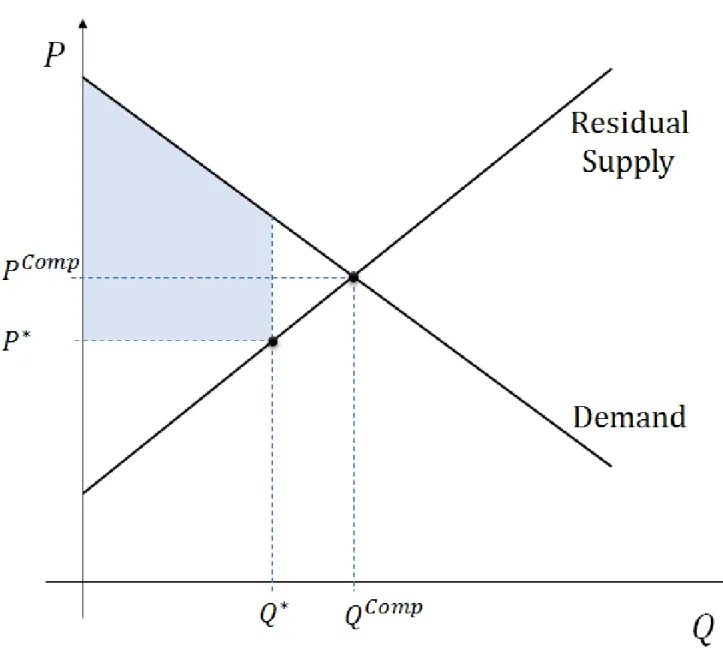
This paper models the strategic behavior of auction participants, and offers model-based
quan-titative benchmarks for assessing the competitiveness and cost-effectiveness of this important
mar-ketplace. Our model builds on the seminal “share auction” model of Wilson (1979) in which bidders
are allowed to submit demand schedules as their bids. This model captures the strategic complexity
of the Treasury’s uniform price auction mechanism very well, and it is in many ways related to
classic models of imperfect competition such as Cournot. In particular, consider a setting (depicted
in Figure 1) where an oligopsonistic bidder with downward sloping demand for the security knows
the residual supply function that she is facing, and is allowed to submit a single price-quantity
point as her bid. Following basic monopsony theory, this bidder will not select the competitive
outcome (Pcomp, Qcomp), which is the intersection of her demand curve and the residual supply
curve. Instead, she has the incentive to “shade” her bid, and pick a lower price-quantity point on
the residual supply curve, such as (P∗, Q∗). This gives her higher surplus (the gray shaded area
below her demand curve up to (P∗, Q∗)) than if she had bid the competitive price and quantity. Of
1Peter Fisher, then Under Secretary of Treasury for Domestic Finance, in a speech titled “Remarks before the Bond
course, the ability of this bidder to “shade” her bid depends on the elasticity of the residual supply
curve she is facing. If this were a small bidder among many others, the residual supply she would
be facing would essentially be flat, allowing for very little ability to bid-shade, as decreasing the
quantity demanded would not result in any appreciable change in the market clearing price. The
optimal bid then is to bid one’s true demand curve.
The Wilson (1979) model, and its generalization that we discuss here enhances this picture by
allowing bidders to have private information about their true demands/valuations for the
securi-ties and to submit more than one price-quantity pair as their bids. This induces uncertainty in
competing bids, and thus an uncertain residual supply curve. What Wilson derives is a locus of
price-quantity points comprising a “bid function” that maximizes the bidder’s expected surplus
against possible realizations of the residual supply curve.
An important assumption of the Wilson setup is that bidders are allowed to bid continuous
bid functions. However, in most real world settings, bidders are confined to a discrete strategy
space that limits the number of price-quantity points they can bid. Indeed, in the auctions that we
study, bidders utilize, on average, 3 to 5 price-quantity points, with a nontrivial fraction of bidders
submitting a single step, making “discreteness” a particularly important problem. To deal with
this issue, we adopt the generalization of the Wilson model by Kastl (2011).
Yet another complication we face in this setting is the fact that bidders have inherently
asym-metric information sets. This asymmetry is introduced by the fact that some bidders (the “primary
dealers”) route the bids of others (the “indirect” bidders), and hence observe a part of the residual
supply curve that other bidders do not. Following our prior work on Canadian treasury auctions
(Horta¸csu and Kastl (2012)) which had a very similar feature, our model also incorporates the
re-duced uncertainty/more precise information that primary dealers possess regarding residual supply.
We develop the model to the point where we can characterize bidders’ optimal decisions in terms
of their (unobserved) “true” demands/marginal valuations, and their beliefs about the distribution
and shape of residual supply. Indeed, the optimality condition closely resembles the inverse
elas-ticity markup rule of classical monopoly theory. The optimality condition thus allows us to infer
as-sumptions regarding bidders’ beliefs. We follow, as in some of our previous work (Horta¸csu (2002),
Horta¸csu and McAdams (2010), Kastl (2011), and Horta¸csu and Kastl (2012)) the seminal insight
of Guerre, Perrigne and Vuong (2000)2 that under the assumption that bidders are playing the
Bayesian-Nash equilibrium of the game, one can use the realized distribution of residual supplies as
an empirical estimate of bidders’ ex-ante beliefs. Once we have the bidders’ beliefs, we can “invert”
the optimality condition to recover bidders’ unobserved demand/marginal valuations rationalizing
their observed behavior.
We then utilize our estimates of bidders’ “behavior-rationalizing” marginal valuations/demand
curves to answer two sets of questions. The first is to quantify the extent of market power exercised
by bidders through bid-shading, as in Figure 1, and how this varies across different subclasses of
bidders. We find that primary dealers shade their bids more than direct and indirect bidders –
which goes towards explaining the observed differences in their bidding patterns (primary dealers
bid significantly lower prices/higher yields than direct and indirect bidders).
The second question we answer is regarding bidder surplus. In Figure 1, one can quantify the
bidder surplus by looking at the area under the bidder’s true demand curve above P∗ and up to
Q∗. Since we have estimates of bidders’ “behavior rationalizing” demand curves, we can calculate this area for each bidder in our data. Our main finding here is that primary dealers, perhaps not
surprisingly, extract more surplus from the auctions than direct or indirect bidders. The magnitude
of the surpluses vary quite a bit between maturity classes, with very little bidder surplus in Treasury
bills, and larger surpluses for Treasury notes.
Our surplus calculations also allow us to connect to a long literature studying the “optimal
auction mechanism” to use to sell Treasury securities. This literature dates at least back Friedman
(1960), who pointed out the bid-shading incentives of bidders in the then-used
discriminatory/pay-as-bid auction utilized by the Treasury, and advocated the use of the uniform-price auction, as it
would alleviate the bid-shading incentive of smaller bidders (for whom bidding one’s valuation is
approximately optimal) and lower their cost of participating in these auctions. However, as noted
by several authors including Wilson (1979) and Ausubel, Cramton, Pycia, Rostek and Weretka
al. (2014) also show that optimal bid shading in these auctions also distorts the efficiency of the
allocations, and thus a general ranking of expected revenues from discriminatory and uniform price
auctions can not be made without knowledge about the specific features of bidder demand.
Given the theoretical vacuum, a variety of empirical approaches have been employed to
as-sess the efficacy of Treasury auction mechanisms. The Treasury’s own study of this question, as
reported by Malvey and Archibald (1998), was based on experimentation with the uniform price
format for 2- and 5-year notes. To assess the revenue properties of the uniform vs. the status-quo
discriminatory format, Malvey and Archibald calculated the auction-when-issued rate spread, and
did not statistically reject a mean difference across the different auction formats. However, they
note that the uniform price auctions “produce a broader distribution of auction awards” across
bidders, and especially a lowered concentration of awards to top primary dealers.
Our empirical approach differs from that of Malvey and Archibald’s and related studies, in that
we do not look at when-issued or secondary market prices to assess the “value” of the securities being
sold.3 Indeed, what we are interested is the “inframarginal surplus” of the bidders, which, in the
presence of downward sloping demand, will not be apparent from looking at market clearing prices
either in the primary or secondary markets. Heterogeneity in valuations that lead to downward
sloping demand for these securities may arise from many different sources: buy-and-hold bidders
may have idiosyncratic portfolio immunization needs, financial intermediaries may attach different
valuations to the Treasuries due to e.g. their use as collateral, primary dealers may value having
an inventory of Treasury beyond its resale value because being a primary creates additional value
streams (such as complementary services or access to Fed facilities).
Recovering the marginal valuations, and thus the surpluses of the bidders allows one to
con-struct an upper-bound to the amount of extra revenue that can be derived from switching the
auction mechanism – as no voluntary participation mechanism can extract more than the entire
surplus that would be obtained in an efficient, surplus-maximizing allocation. We find that the
re-alized total bidder surplus in these auctions amounts to about 3 basis points for the average auction
(though surpluses are appreciably higher for Notes auctions than they are for Bills auctions). We
3When we looked at the differential between auction-close when-issued rates and the auction stop-out rate, we
also estimate the extent of inefficiency of the allocation to be approximately 2 basis points. These
findings suggest that the most cost-savings one can hope for from a redesign of the auction
mech-anism will be around 5 basis points. Of course, any incentive compatible and individually rational
mechanism needs to allow some surplus for the bidders; thus, this is an extremely conservative
upper bound.
The paper proceeds in the following manner. In Section 2, we describe our data, which covers
auctions conducted between July 2009 and October 2013, and the main characteristics of the U.S.
Treasury auction system. We then provide brief summary descriptions of allocation and bidding
patterns in the data by different subclasses of bidders. Section 3 develops our model of bidding that
incorporates the salient features of the U.S. Treasury auction system, and discusses the optimality
conditions that underlie our empirical strategy. Section 5 presents the results regarding bid shading
and bidder surplus.
2
Description of our Data Sample and Institutional Background
The data sample used in this study comprises of 975 auctions of Treasury securities conducted
between July 2009 and October 2013 (Table 6). The securities in our sample range from 4 week
bills to 10 year notes, with 822 auctions of 4-week, 13-week, 26-week, 52-week bills and cash
management bills, and 153 auctions of 2-year, 5-year, and 10-year notes. The total volume of
issuance through these auctions was 27.3 trillion US dollars, with the average issue size around 28
billion dollars.
The issuance mechanism is a sealed-bid uniform-price auction, which has been the preferred
auction mechanism of the Treasury since October 1998. Bids consist of price-quantity schedules and
define step functions, with minimum price increments of 0.5 basis points for thirteen, twenty-six,
fifty-two week, and cash management bills and 0.1 basis points for all other securities.
Noncompet-itive, price-taking bids are also accepted but are limited to $5 million and are usually due before
noon, an hour earlier than competitive bids. Noncompetitive bid totals are announced prior to the
deadline for competitive tenders.
indirect bidders. During the sample period, 17 to 21 primary dealers regularly bid in the auctions
and made markets in Treasury securities. These primary dealers can bid on their own behalf (“house
bids”) and also submit bids on behalf of the indirect bidders. Primary dealers are, as a class of
bidders, the largest purchasers of primary issuances. In terms of tendered quantities, primary dealer
tenders comprise 69% to 88% of overall tendered quantities. Direct bidders tender 6% to 13% and
Indirect bidders 6% to 18% of the tenders.4 In terms of winning bids, or allocated quantities, we
find that Primary Dealers tend to win a smaller proportion of their tendered quantities. Primary
Dealers are allocated between 46% to 76% of competitive demand, while Indirect Bidders win the
disproportionate share of 17% to 38%, with Direct Bidders’ allocation shares staying close to their
tendered quantity shares. Let us now analyze these bidding differences more closely.
2.1 Analysis of Bid Yields and Bid Quantities
The fact that Primary Dealers are winning a smaller share of their tenders than Direct and Indirect
Bidders suggests that Primary Dealers bid systematically higher (lower) yields (prices) in these
auctions. To investigate this further, Table 6 reports the quantity-weighted bid-yields submitted
by the three bidder groups across different maturities. We include the within-auction standard
deviation of quantity-weighted bid yields as a measure of bid dispersion within bidder group. Since
bids in these auctions are effectively in the form of demand curves, we also include the total tender
quantity submitted by a bidder as a percentage of the issue size (%QT), and the percentage of her
tender quantity that the bidder won (%Win).
Looking at the (quantity-weighted) bid yields we see the clear pattern, across all maturities,
that Primary Dealers systematically place higher (lower) bid yields (prices) than Direct and Indirect
Bidders. The gap in bid yields between Primary Dealers and Indirect Bidders is quite substantial,
and ranges between 3 to 18 basis points depending on maturity. Primary Dealers also appear to
4Earlier analyses of similar tender and allocation shares by bidder classes have been performed by Garbade and
be bidding 2 to 8 basis points higher yields than Direct Bidders for maturities, except for 2 year
notes.
The within-auction dispersion of (quantity-weighted) bid-yields across Primary Dealers is very
similar to the dispersion of Direct Bidder bids, ranging from 2 to 7 basis points. Indirect Bidders
submit more dispersed bids, especially for the longer-term securities, with the dispersion rising to
19 basis points for 10 year bond auctions.
Primary dealers bid for much larger quantities. The average Primary Dealer offers to purchase
between 10% to 20% of issuance, while Direct bidder quantity tenders hover between 3-5% and
Indirect Bidders’ tenders between 1-3% of the issuance. Given that Primary Dealers tend to bid
higher yields, however, it is not surprising that Primary Dealers get allocated a smaller share of
their total tenders than Direct or Indirect Bidders. Indeed, while Primary Dealers end up winning
only about 20% of their tendered quantities, Direct Bidders win 40-50% and Indirect Bidders,
70-80%.
In Table 3, we accounted for how the quantity-weighted bids compare to the US Treasury
published yield (of the respective maturity) on the day of the auction. It is evident that indirect
bidders systematically bid lower yields than the market-level prevailing yield (and substantially
so in auctions of 6-month Tbills), the direct bidders bid about at the prevailing yields and the
primary dealers bid on average above these yields. Of course these numbers per se are hard to
interpret, since there might be other effects at play that are not visible when looking just at the
quantity-weighted bids. For example, if primary dealers need to absorb much larger amounts of the
auctioned instruments (recall that they have to bid for NP D1 share of the supply), they will need
to be compensated for this and hence their bids might reflect this compensation even in absence of
any market power or direct price effect considerations.
2.2 Drivers of Bid Differentials?
What might drive these bid differentials across bidder groups? These different bidder groups
have different demand/willingness-to-pay for these securities, depending on their idiosyncratic
port-folios, while others are broker-dealers whose primary purpose is resale. In particular, it is possible
that the reason why Primary Dealers bid lower (higher yields) is that they systematically have
lower demand/willingness-to-pay for the securities than other bidder classes.
Another possibility is the exercise of market power. Even if bidders’ willingness-to-pay is the
same for the securities, the Primary Dealers, as we see, are much larger players in this market,
commanding significant market share. Such buyers may be able to exercise their monopsony power
to try to lower the marginal cost of acquisition.
A particularly detrimental source of market power leading to higher yields bids, of course, is
collusion among primary dealers. Following the recent settlements in the LIBOR fixing scandal
and the Foreign Exchange rate fixing case, there have, indeed, been a number of recent allegations
regarding collusive behavior among primary dealers in the treasury auctions as well.5 However, the
raised allegations regarding misconduct have been about information sharing between the primary
dealers; one particular allegation is that primary dealers communicated about the amount of
cus-tomer/indirect bidder interest they were receiving prior to the auction. Such information sharing
does not necessarily lead to coordinated conduct; indeed, sharing information about private
val-ues/costs prior to an auction can lead to potentially stiffer competition a la Bertrand compared to
the private information case. Nevertheless, our model, which we describe below, can be tailored to
take into account the precise nature of such information sharing arrangements.
Yet another possibility for the high-yield/low-price bids by the Primary dealers is the fact that
they face minimum bid constraints. The Treasury expects primary dealers to bid in every auction,
and to bid, at a minimum, for their pro-rata share of the auction volume based on the number of
primary dealers at the time of the auction. However, in our data, we find primary dealers to be
bidding quantities close to their pro-rata share only very infrequently – in our entire data set, there
are only 23 instances (out of 19,000 bids) in which a primary dealer bid for a quantity that is within
1% of its minimum bidding requirement. This suggests that the minimum bidding requirement is
only very rarely binding.
Table 4 investigates the differentials in bid yields implied by Table 6 through regressions. We
5See, for example,
have split the sample into auctions of Treasury Bills and Treasury Notes, as it is possible that the
market dynamics are very different across these different classes of securities. We also control for
auction fixed effects in each regression; thus the regressions provide within-auction comparisons
that account for differing supply-demand conditions that affect the level of the bids.
The first and third specifications regress (quantity-weighted) bid yield on indicators for Direct
and Indirect Bidders in the Bills and Notes sectors. We find here the pattern implied by Table 6:
Primary Dealers systematically (and statistically significantly) bid higher yields than Direct and
Indirect Bidders. Primary Dealer bids are 2 (4) basis points higher than Direct (Indirect) bids in
the Bills sector, and 6 (11) basis points higher in the Notes sector.
The second and fourth columns of Table 4 include the bidder’s share of the total tender size as
a proxy for bidder size. There are two main ways through which bidder size may affect the bids:
bidders demanding larger quantity may have higher demand for the security, but they may also
have higher market power. The regressions indicate that larger bidders systematically bid higher
yields. The effect is quite large – the coefficient estimate indicates that a size increase of 10% of
total issue size accounts for 1(6) basis point increase in the bid yield.
Accounting for bidder size appears to lower the differences in bid yields across bidder classes,
but Primary Dealers appear to bid higher yields than Direct and Indirects even accounting for their
offer share of the total issue.
As we noted above, since bids reflect both differences in demand and also differences in market
power, it is difficult to interpret these documented differences in bids. Even though we find that
larger bidders bid higher yields, this is not prima facie evidence that large bidders exercise market
power; it is possible that larger bidders also have lower demand.
In the next section, we will describe a model of bidding that will allow us to separate out the
market power and demand components of bid heterogeneity. The model, and the measurement it
will allow us to conduct, willrely on the assumption of bidder optimization. In essence, what we will
end up doing is to measure the elasticity of (expected) residual supply faced by each bidder. This
is directly observable in the data, and does not require behavioral assumptions. This elasticity will
are expected profit maximizers who will exercise their market power in a unilateral, noncooperative
fashion, we can then estimate the willingness-to-pay/demand that rationalizes the observed bid.
3
Model of Bidding
Our analysis is based on the share auction model of Wilson (1979) with private information, in
which both quantity and price are assumed to be continuous. Wilson’s model was modified to
take into account the discreteness of bidding (i.e., finitely many steps in bid functions) as in Kastl
(2011). In Horta¸csu and Kastl (2012), we further adapted this model to allow primary dealers to
observe the bids of others, hence allowing for “indirect bidders,” whose bids are routed by primary
dealers.
Formally, suppose there are three classes of bidders: NP primary dealers (in index set P), NI
potential indirect bidders (in index set I) and ND potential direct bidders (in index set D). They
are each bidding for a perfectly divisible good of (random) Q units. We assume that the number
of potential bidders of each type participating in an auction, NP, NI, ND, is commonly known.
However, except primary dealers, the exact number of indirect and direct bidders is not known.
Before the bidding commences, bidders observe private (possibly multidimensional) signals. Let
us denote these signals for the different bidder groups as S1P, ..., SNP
P, S
i
1, ..., SNII, S
D
1 , ..., SNDD. The
bidding then proceeds in two stages. In stage 1, indirect bidders submit their bids to their primary
dealer. These bids, denoted byyI
p|SjI
, specify for each pricep, how big a share of the securities
offered in the auction indirect bidderjdemands as a function of her private informationSI
j. In stage
2, direct bidders submit their bids,yDp|SD j
, and primary dealerk submits her customers’ bids,
and also places her own bid, yP p|SP k, ZkP
, where ZP
k contains all information dealer k observes
from seeing the bids of its customers. If dealer k observes the bids of not only her customers but
also of other dealers’, as has been recently alleged, one can appropriately modify the information
set of this dealer.
We will impose the following additional assumptions:
Assumption 1 Direct and indirect bidders’ and dealers’ private signals are independent and drawn
with strictly positive densities.
Strictly speaking, independence is not necessary for our characterization of equilibrium behavior
in this auction, but we impose it in our empirical application.
Winning q units of the security is valued according to a marginal valuation function vi(q, Si).
We assume that the marginal valuation function is symmetric within each class of bidders, but
allow it to be different across bidder classes. We will impose the following assumptions on the
marginal valuation function vg(·,·,·) forg∈ {P, I, D}:
Assumption 2 vg(q, Sig) is non-negative, measurable, bounded, strictly increasing in (each
com-ponent of ) Sig ∀q and weakly decreasing inq ∀sgi, for g∈ {P, I, D}.
Note that this assumption implies that learning other bidders’ signals does not affect one’s own
valuation – i.e. we have a setting with private, not interdependent values. This assumption may
be more palatable for certain securities (such as shorter term securities, which are essentially cash
substitutes) than others, but is the most tractable one under which we can pursue the “demand
heterogeneity” vs. “market power” decomposition. Note that under this assumption, the additional
information that a primary dealer j possesses due to observing her customers’ orders, ZjP, simply
consists of those submitted orders. As will become clear below, this extra piece of information allows
the primary dealer to update her beliefs about the competitiveness of the auction, or, somewhat
more precisely, the distribution of the market clearing price.6
To ease notation, letθj denote private information of bidderj, i.e., for a direct bidderθj ≡SDj ,
indirect bidderθj ≡SjI and for a primary dealer θj ≡
SP j , ZjP
.
Bidders’ pure strategies are mappings from private information in each stage to bid functions
σi : Θi → Y, where the set Y includes all admissible bid functions. The expected utility of type
θi-bidder (from group g ∈ {P, D, I}) who employs a strategy yig(·|θi) in a uniform price auction
6In Horta¸csu and Kastl (2012), we were able to test this assumption by exploiting the unique feature of Canadian
given that other bidders are using nyj(g,−g)(·|·)o
j6=i can be written as:
EUig(θi) = EQ,Θ−i|θiu
g(θ i,Θ−i)
= EQ,Θ−i|θi "
Z Qci(Q,Θ,y(g,−g)(·|Θ)) 0
vig(u, θi)du−Pc
Q,Θ,y(g,−g)(·|Θ)QicQ,Θ,y(g,−g)(·|Θ)
#
whereQci Q,Θ,y(g,−g)(·|Θ)
is the (market clearing) quantity bidderiobtains if the state (bidders’
private information and the supply quantity) is (Q,Θ) and bidders bid according to strategies
spec-ified in the vector y(g,−g)(·|Θ) = hyg1(·|Θ1 =θ1), ..., y|G|g ·|Θ|G|=θ|G|
, ..., y|−G|−g ·|Θ|−G| =θ|−G|i
.
SimilarlyPc Q,Θ,y(g,−g)(·|Θ)
is the market clearing price associated with state (Q,Θ). In other
words, the expected utility is the expected consumer surplus, as given by the expected area under
the demand curve up to the random allocation, Qci, minus the expected payment, which depends
on the random allocation and random market clearing price, Pc.
Our solution concept will beBayesian Nash Equilibrium, which is a collection of bid functions
fromY, such that for every groupg∈ {P, D, I}, and almost every typeθi of bidderifromgchooses
this bid function to maximize her expected utility: ygi (·|θi) ∈arg maxEUig(θi) for a.e. θi and all
biddersi and all groupsg.
We will assume that the bidding data is generated by agroup symmetric Bayesian Nash
equilib-rium of the game7 in which direct and indirect bidders submit bid functions that are symmetric up
to their private signals, i.e. yD j
p|SD j
=yDp|SD j
, j ∈ D, and yI j
p|SI j
=yIp|SI j
, j ∈ I.
Primary dealers also bid in an ex-ante symmetric way, but up to their private signaland customer
information, i.e. yjPp|SjP, ZjP=yPp|SjP, ZjP, j∈ P.
Bidders’ choice of bidding strategies is restricted to non-increasing step functions with an upper
bound on the total quantity they can win (up to 35% of the total quantity). When bidders use
step functions as their bids, rationing occurs except in very rare cases. We will thus assume, as
it is in practice, pro-rata on-the-margin rationing, which proportionally adjusts the marginal bids
so as to equate supply and demand. Also, in extremely rare situations where multiple prices clear
the market (due to discreteness of quantities), we assume that the auctioneer selects the highest
market clearing price.
3.1 Characterization of equilibrium bids
We realize that Bayesian Nash equilibrium play may appear like a very strong behavioral
assump-tion to impose on bidders at the outset. However, what is needed for our empirical strategy to
work is “best response” or expected utility maximization behavior by bidders, and the ability for
the econometric analyst to reconstruct the uncertainty faced by the bidders. The equilibrium
as-sumption posits that bidders have rational expectations about realized, ex-post outcomes – which
then allows the econometrician to use data on realized outcomes to recreate the information sets
of bidders.
The key source of uncertainty faced by the bidders in the auction is the market clearing price,Pc,
which maps the state of the world, sI,sD,sP,zinto prices through equilibrium bidding strategies.
Let us now define the probability distribution of the market clearing price from the perspective
of a direct bidderj, who is preparing to make a bidyD(p|sj). The probability distribution of the
market clearing price from the perspective of direct bidderj will be:
Pr (p≥Pc|sj) =E{S
k∈D∪P∪I\j,Zl∈P}I Q−
X m∈P
yP(p|Sm, Zm)− X l∈I
yI(p|Sj)− X k∈D\j
yD(p|Sk)≥yD(p|sj)
(1)
where E{·} is an expectation over all other bidders’ (including indirect bidders, primary dealers,
and other direct bidders) private information, and I(·) is the indicator function.
This expression says that the probability that the market clearing pricePcwill be below a given
price level p is the same as the probability that residual supply of the security at price p will be
higher than the quantity demanded by bidderjat that price. In the expression inside the indicator
is the residual supply function faced by bidder j. This residual supply function is uncertain from
the perspective of the bidder, but its distribution is pinned down by the assumption that the bidder
knows the distribution of its competitors’ private information and the equilibrium strategies they
employ.
For a primary dealer, the distribution of the market clearing price is slightly different, since
the dealer will condition on whatever information is observed in the indirect bidders’ bids. In
the market clearing price from the perspective of primary dealerj, who observes the bids submitted
by indirect biddersm in an index setM|, is Pr (p≥Pc|sj, zj), and equal to:
E
Sk∈I\M|,Sl∈D,Sn∈P\jZn∈P\j|zj
I
Q− X
k∈I\M|
yI(p|Sk)−
X
l∈D
yD(p|Sl)−
X
n∈P\j
yP(p|Sn, Zn)≥yP(p|sj, zj) +
X
m∈M|
yI(p|sm)
The main difference in this equation compared to equation (1) is that the dealer conditions on all
observed customers’ bids, all bids in index setM. This is exactly where the dealer “learns about
competition” – the primary dealer’s expectations about the distribution of the market clearing
price are altered once she observes a customer’s bid.8
Finally, the distribution of Pc from the perspective of an indirect bidder is very similar to a direct bidder, but with the additional twist that the indirect bidder recognizes that her bid will be
observed by a primary dealer, m, and can condition on the information that she provides to this
dealer. The distribution of the market clearing price from the perspective of an indirect bidderj, who submits her bid through a primary dealerm is given by:
Pr (p≥Pc|sj) =
E{Sk∈I\j,Sl∈D,Sn∈PZn∈P|sj}I
Q− X
k∈I\j
yI(p|Sk)−
X
l∈D
yD(p|Sl)−
X
n∈P
yP(p|Sn, Zn)≥yI(p|sj)
where yI(p|sj)∈Zm.
Given the distributions of the market clearing price defined above (which, in a Bayesian Nash
Equilibrium, coincide with bidders’ beliefs), a necessary condition for optimal bidding is given by
below:
Proposition 1 (Kastl 2012) Under assumptions 1 and 2, in any Bayesian Nash Equilibrium of a
Uniform Price Auction, for a bidder of type θi submitting Kˆ(θi) steps, every step (qk, bk)
charac-terizing the equilibrium bid function y(·|θi) has to satisfy:
vi(qk, θi) =E(Pc|bk> Pc > bk+1, θi) +
qk
Pr (bk> Pc > bk+1, θi)
∂E(Pc;b
k ≥Pc ≥bk+1, θi)
∂qk
(2)
8Once again, if primary dealers engage in information sharing about their customer bids, as has been alleged
∀k≤Kˆ (θi) such that v(q, θi) is continuous in a neighborhood of qk.
Note that this expression is very close to M C = E[P(Q)] +E[P′(Q)]Q, i.e., to an oligopolist’s
optimality condition in a setting where the oligopolist faces uncertain demand in the spirit of
Klemperer and Meyer (1989).
An interesting implication of Equation (2) pointed out by Kastl (2011) is that bids above
marginal values may be optimal in a uniform price auction with restricted strategy sets. The
intuition has to do with the restriction on the strategies requiring the bidders to “bundle” bids
for several units together and thus to trade-off potential (ex post) loss on the last unit in the
bundle against the probability of obtaining the high-valued infra-marginal units in the bundle.
For example, consider one very small bidder, so that he is a “price taker.” Assume also a
non-degenerate distribution of the market clearing price with continuous and strictly positive density
over a compact support and let Ki = 1; i.e. the bidder is constrained to submit a single step as
her bid. In this case, the second term on the RHS of (2) vanishes because of the bidder being a
price taker. This bidder thus optimally asks for a quantity such that his marginal valuation at
that quantity is equal to the expected price conditional on this price being lower than his bid, i.e.
vi(qk, θi) = E(Pc|bk> Pc, θi). Therefore, whenever there is a positive probability of the market
clearing price being below his bid, his bid will be higher than his marginal valuation for that
quantity.
For our empirical exercise, it will be useful to define the notion of bid-shading based on the
above condition for optimal bidding. Typically, bid-shading is defined as the difference between
a bidder’s value and her bid. As highlighted above, however, this notion of shading might often
result in negative values in auctions where bids are constrained to be step functions. The reason is
that, especially in very competitive auctions, bidders would submit bids such that their marginal
value is equal to the expected market clearing price conditional on that price being lower than this
bid and conditional on this bid being the marginal bid of this bidder.
Definition 1 The average bid shading is defined as: B(θi) =
PKi
k=1qk[vi(qk,θi)−bk]
PKi k=1qk
.
course, be positive on the inframarginal units. A negative value is due to the combination of two
factors: (i) the perceived market power of this bidder at kth step is probably small and (ii) this
bidder believes that if kth step were marginal, the market clearing price will likely be much lower
than her bid.
Given equation (2) a perhaps more natural notion of shading that only takes positive values is
the following:
Definition 2 The average shading factor is defined as: S(θi) =
PKi
k=1qk[vi(qk,θi)−E(Pc|bk>Pc>bk+1,θi)]
PKi k=1qk
.
This is a quantity-weighted measure of shading, where shading at stepkis defined as the difference
between the marginal value, vi(qk, θi) and the expected market clearing price, conditional on kth
step being marginal, E(Pc|bk > Pc> bk+1, θi). Inspecting equation (2), it is straightforward to
see that this measure of shading is non-negative, since market clearing price is non-decreasing in
quantity demanded. Another way to interpret this shading factor is to note that it corresponds to
the weighted sum of the second term on the right-hand side of equation (2), which is essentially
the expected inverse elasticity of the residual supply curve faced by the bidder.
4
Estimating Marginal Valuations
To estimate the rationalizing marginal valuations, we use the “resampling” method developed in
Horta¸csu (2002), Kastl (2011), and Horta¸csu and Kastl (2012). The asymptotic behavior of our
estimator is described in detail in Horta¸csu and Kastl (2012) and Cassola, Horta¸csu and Kastl
(2013). The “resampling” method that we employ is to draw from the empirical distribution of
bids to simulate different realizations of the residual supply function that can be faced by a bidder,
thus obtaining an estimator of the distribution of the market clearing prices. Specifically, in the case
whereall N bidders are ex-ante symmetric, private information is independent across bidders and
the data is generated by a symmetric Bayesian Nash equilibrium, the resampling method operates
as follows: Fix a bidder. From all the observed data (all auctions and all bids), draw randomly (with
replacement)N−1 actual bid functions submitted by bidders. This simulates one possible state of
results in one potential realization of the residual supply. Intersecting this residual supply with the
fixed bidder’s bid we obtain a market clearing price. Repeating this procedure a large number of
times we obtain an estimate of the full distribution of the market clearing price conditional on the
fixed bid. Using this estimated distribution of market clearing price, we can obtain our estimates
of the marginal value at each step submitted by the bidder whose bid we fixed using (2).
In the present case, we have three classes of bidders: NP primary dealers (in index setP),NI
potential indirect bidders (in index set I) and ND potential direct bidders (in index set D). In
this context, the resampling algorithm should be modified in the following manner: to estimate
the probability in equation (1) for direct and indirect bidders, we draw direct and indirect bids
from the empirical distribution of these classes of bids (we augment the data with zero bids for
non-participating direct and indirect bidders). Now, to account for the asymmetry induced across
primary dealer bids due to the observation of customer signals, we condition on each indirect
bid, yI(p, Sj) by drawing from the pool of primary dealer bids which have been submitted having
observed a “similar” indirect bid. Also, to estimate the probability distribution from the perspective
of primary dealers, we need to take into account the full information set of the dealer. This is
achieved by a slight modification of the above procedure: fixing a primary dealer, who has seenM
indirect bids, we draw NI −M, rather than NI, indirect bids, and take the observed indirect bid
along with the dealer’s own bid as given when calculating the market clearing price, i.e., we subtract
theactual observed customer bid from the supply before starting the resampling procedure.
Unobserved heterogeneity across auctions that may be driving valuations is a big concern in
the empirical auctions literature. The danger this creates is the potential pooling of bidding data
across auctions that have very different demand structures, which may cloud inference regarding
the probability distribution of the market clearing price. Another, related, concern is the potential
for multiple strategic equilibria – bidders may be playing different equilibria in different auctions
in the data set. To combat these issues, we use marginal valuations auction-by-auction; using data
on bids from only one auction at a time. While this reduces precision of our estimates, the volatile
economic environment especially in 2009 and 2010 suggests that auctions of the same security
unobservables at the auction level may be very important. We discuss the consistency property of
the single-auction estimation scheme in Cassola, Horta¸csu and Kastl (2013).9
Using this modified resampling method we can therefore obtain an estimate of the distribution
of market clearing price from the perspective of each bidder. Inspecting equation (2), the only
other object we need to estimate is the slope of the unconditional expectation. We estimate this
using the standard numerical derivative approach. In particular, for each bidder we use the same
resampling approach described earlier to estimate E(Pc|bk ≥Pc ≥bk+1), which together with an
estimate of Pr (bk≥Pc ≥bk+1) and Bayes’ rule yields an estimate of E(Pc;bk≥Pc ≥bk+1). Call
this estimate ERT (Pc;bk ≥Pc ≥bk+1), where T indexes the sample size (the number of auctions)
and R stands for the resampling estimator. To obtain an estimate of the numerical derivative
of this expectation with respect to quantity demanded at step k we perturb qk in the submitted
bid vector to some qk−εd and obtain an estimate of ERT (Pc;bk≥Pc ≥bk+1) conditional on the
perturbed bid vector. We can then construct the estimator of the derivative:
∂ERT (Pc;bk≥Pc ≥bk+1)
∂qk
= E
R
T (Pc;bk ≥Pc ≥bk+1, qk)−ETR(Pc;bk≥Pc ≥bk+1, qk−εd)
εd
where {εd}∞d=1 is a sequence converging to zero. One difficulty when estimating the slope of this
expectation w.r.t. qk is choosing the appropriate neighborhoodεdso that the numerical derivative
is a consistent estimate. Loosely speaking, this neighborhood should shrink to zero as the sample
size increases. Pakes and Pollard (1989) establish that with a regularity condition (on uniformity),
such an estimator is consistent whenever T−12ε−1 =Op(1), i.e., whenever εdoes not decrease too
fast as the sample size increases.
9Utilizing auction-by-auction estimation also allows our estimates to account for the recent
5
Results
5.1 Bid Shading Analysis
As we discussed in our analysis of bids, the difference in bids across bidder groups may arise from
two separate factors: differential ability to exercise market power, i.e. bid shading, vs. differential
willingness-to-pay for the issued security. Our estimation method yields estimates of the two terms
on the right hand side of Equation (2) based on the empirical distribution of bids within each
auction in our data set. Using these, we can construct an estimate of the marginal valuation for
each bid step, which can then be utilized to compute the two different shading factors we defined
in the previous section for each bidder and auction.
Table 6 reports the results of regressions similar to those for bids. The first two columns of the
table look at the differences in bid shading (according to Definition 1 above) across bidder groups
for the Bill sector. Column (1) implies that Primary Dealers shade their bids 1.9 basis points more
than Direct Bidders, and 3.5 basis points higher than Indirect Bidders. Column (2) introduces the
bidder size control, and we find that the shading differentials decline slightly, to 1.4 basis point
against Direct Bidders and 3 basis points against Indirect Bidders. We also find, intuitively, that
larger bidders choose to shade their bids more. The coefficient estimate suggests that going from
zero to 10% market share is associated with 0.3 basis points more bid shading.
Columns (3) and (4) repeat the same analysis for Definition 2 of bid shading, and find
qualita-tively the same result.
Columns (5) through (8) repeat the analysis for the Notes sector. Here, we see even larger
differentials in shading. Primary Dealers shade their bids (according to Definition 1) 5 basis points
more than Direct Bidders and 13 basis points more than Indirect Bidders. Putting in the control
for bidder size, once again we find that larger bidders can shade their bids more: going from zero
to 10% market share increases shading by 3 basis points. The size control diminishes the shading
differential between Primary Dealers and Direct and Indirect Bidders (to 2 and 10 basis points),
but, once again, does not eliminate the differential. Once again, Columns (7) and (8) repeat the
Demand Differentials or Bid-Shading Differentials?
Recall that our analysis of bids in Table 4 revealed that, controlling for size, Primary Dealers
bid 1 (2.5) basis points higher yields than Direct(Indirect) bidders for Bills, and 1 (4) basis points
higher yields for Notes. Since we found that Primary Dealers shade their bids 1.4 (3) basis points
more than Direct (Indirect) for Bills, and 2(10) basis points more than Direct (Indirect) bidders
for Notes, the bid differentials are rationalized by Primary Dealers having 0.4 (0.5) basis points
higher willingness-to-pay for Bills, and 1 (6) basis points higher willingness-to-pay for Notes – again,
controlling for bidder size. I.e., our results suggest that, under the assumption of expected profit
maximization, the main reason why Primary Dealers bid higher yields than other bidder groups is
not because they have lower valuation for the securities, but because they are able to exercise more
market power.
5.2 Infra-marginal Surplus Analysis
A question related to bid-shading that we can answer through our analysis is to quantify how much
infra-marginal surplus bidders are getting from participating in these auctions. Once again, we
can utilize Equation (2) to calculate the bidders’ marginal valuations, and use these to compute
ex-post surplus each bidder gains on the units that they win in the auction. To compute surplus, we
obtain point estimates of the “rationalizing” marginal valuation function v(q, s) at the (observed)
quantities that the bidders request. We then compute the area under the upper envelope of the
inframarginal portion of the marginal valuation function, and subtract the payment made by each
bidder.
We should provide abundant caution regarding what “infra-marginal bidder surplus” means.
Any counterfactual auction system would also have to allow bidders to retain some surplus. Indeed,
in Figure 1, we see very clearly that even if bidders bid perfectly competitively, i.e. reveal their true
marginal valuations without any bid shading, they would gain some surplus from the auction, just
because they have downward sloping demand curves. Indeed, if there are any costs of participating
in the auction, it would have to be justified by the expected surplus. In terms of assessing the cost
efficient allocation reflects a conservative upper bound to the amount of cost-saving that can be
induced by a change in issuance mechanism.
With the above qualifications, Table 6 reports the infra-marginal surpluses enjoyed by different
bidders groups across the maturity spectrum. We report the surpluses in basis points, and also
report the total infra-marginal surpluses accrued to the bidders during our sample period of July
2009 to October 2013.
Direct and Indirect bidder surpluses are between 0.02 and 3.58 basis points across the maturity
spectrum, with the shorter end of the maturity spectrum generating very low surpluses in general.
Once again, these surpluses may reflect the outside option of not buying these securities in auction
and purchasing them in the when-issued or resale markets – and appear sensible given the
differen-tials between auction prices and secondary market rates. Aggregating the surpluses over the entire
set of auctions in our data set (which amounted to about $27 trillion in issue size), we find Direct
and Indirect Bidders’ aggregate surplus to be about $1.6 billion, or about 0.6 basis points.
Primary Dealers’ infra-marginal surplus, however, appears to be significantly larger. For
Pri-mary Dealers, the derived surplus might not necessarily be in line with the differentials with the
quoted secondary market prices of these securities. Primary Dealers’ demand is typically quite
large, and fulfilling such levels of demand is likely to have a price impact in the secondary markets.
Moreover, retaining Primary Dealership status has a number of complementary value streams
at-tached to it beyond the profits derived from reselling the new issues. For example, being a Primary
Dealer allows firms access to open market operations and, especially in this period, the QE
auc-tion mechanism that is exclusive to primary dealerships. Between March 2008 and February 2010,
Primary Dealers also had access to a special credit facility from the Fed to help alleviate liquidity
constraints during the crisis. Indeed, compared to Primary Dealers, we may expect the surpluses
attained by Direct and Indirect bidders to be more closely aligned with their outside options of
purchasing these securities from secondary markets.
We find that Primary Dealers derive most of their infra-marginal surplus from the longer end (2
to 10 year notes) of the maturity spectrum. There may be a number of reasons why demand for this
of different portfolio needs across dealers’ clientele. Moreover, there are typically alternative uses
for such securities beyond simple buy-and-hold – Duffie (1996) shows that this part of the spectrum
can be particularly valuable for its use as collateral in repo transactions. Surpluses derived from
the shorter end of the maturity spectrum, which may have fewer alternative uses, are much smaller.
Overall, we find that Primary Dealers’ derived surplus aggregated to $6.3 billion during our
sample period. Compared against the $27 trillion in issuance, Primary Dealer surplus makes up
for 2.3 basis points of the issuance. Along with the Direct Bidder and Indirect Bidder surpluses,
we find that bidder surplus added up to 3 basis points during this period.
Once again, we should emphasize that any other issuance mechanism would have to provide
bidders with surpluses to ensure participation and to reward them for their private information.
Moreover, even if bidders are behaving in a perfectly competitive manner, without displaying any
bid-shading, they would enjoy surpluses. However, we can conservatively estimate that revenue
gains from further optimizing the issuance mechanism is bounded above by 3 basis points.
Table 7 runs regressions on the calculated bidder surpluses that closely resemble those in Tables 4
and 6. The surpluses here are reported in thousands of dollars, and all regressions control for auction
fixed effects, giving us within auction comparisons. In Column (1), we find that Direct and Indirect
bidders gain significantly lower surpluses than Primary Dealers (the excluded category appearing
in the constant), and that Indirect bidder surplus especially is not statistically different from zero.
Column (2) adds in the bidder size control, measured as the bidder’s tender size as percentage
of total supply (% Q Total). We find that larger bidders indeed gain higher surpluses. However,
Direct and Indirect Bidders gain lower surpluses than Primary Dealers even when size is controlled
for.
Column (3) introduces a new control variable – we have added here the number of Indirect
Bidders whose bids a Primary Dealer routes in the auction. This variable is a rough proxy for
the order-flow information that the Primary Dealer is privy to. Indeed, the regression reveals a
significant correlation between the number of Indirect Bidders who routed their bids through a
Primary Dealer, and the surplus (controlling for the bidder’s size). An additional Indirect Bidder
surplus.
Columns (4) through (6) repeat the same analysis for the Notes sector. We note that the implied
Primary Dealer surplus in this sector (which is measured by the constant term in our regression) is
much larger as compared to their surplus in Bills auctions. Direct and Indirect Bidders gain much
smaller surpluses compared to the Primary Dealers – indeed, Indirect Bidder surplus is very close
to zero.
When we control for bidder size in Column (5), we find a very large benefit to being large.
An increase in market share from 0 to 10% of the issue size is correlated with a rise in surplus of
$830k in the Notes auctions. Once again, though, we should stress that this is not necessarily due
to market power. It is very possible that larger bidders also have higher demand, and thus derive
more surplus from the auctions.
Finally, we introduce the number of Indirect Bidders routed by Primary Dealers in Column
(6). Here, we find that each additional Indirect Bidder observed is associated with a $200K gain
in Primary Dealer surplus. Since Primary Dealers on average route 2.5 Indirect Bids in Notes
auctions, this estimate suggests that we can ascribe about $500K or about 25% of their surplus
in Notes auctions to information contained in Indirect bids. However, we should note that there
are important caveats to interpreting this as the “value of order flow.” It is possible that Primary
Dealers who observe more Indirect bids may have systematically higher valuations for the securities,
and hence may be getting higher surpluses due to this.10
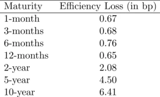
5.3 Efficiency
Using our estimates of marginal values, we can compute the efficient surplus. In particular, fixing
the supply in an auction, we can construct a measure of efficiency by comparing the surplus from
the efficient allocation to the surplus that is achieved in the actually implemented allocation. Our
efficiency estimates are reported in Table 8. Overall, the efficiency losses seem to be quite modest,
amounting to just over 2 basis points on average. It seems that especially on the shorter side of
10In our prior work on Canadian Treasury auctions (Horta¸csu and Kastl (2012)) we focused on revisions of primary
the maturity spectrum the auctions are quite efficient. In auctions of bills, only rarely does the loss
exceed 1 basis point. This is likely a consequence of bidders submitting very similar (and flat) bids
in these short-term auctions. Therefore, any possible misallocation does not have consequences
that would be too bad for total surplus. On the other hand, at long maturities, the efficiency loss
is slightly higher - up to 6.4 basis points in 10-year notes auctions. The somewhat larger loss here
is driven by the much larger heterogeneity of expressed bids in these auctions.
6
Conclusion
We have analyzed a unique and detailed data set to study bidding behavior in a large sample of
U.S. Treasury auctions conducted between July 2009 and October 2013. We have documented
sig-nificant differences in bidding behavior across the three different bidder groups: Primary Dealers,
Direct Bidders, and Indirect Bidders. We provide a modelling framework to decompose the bidding
differentials into differences in demand/willingness to pay, and differences in ability to exercise
mar-ket power. We estimate marmar-ket power by assuming optimizing behavior and rational expectations
about the elasticity of residual supply. Our results suggest that opportunities to exercise market
power do exist in this market, and that Primary Dealers especially have the potential to shade their
bids significantly – to the extent that their bids are lower (higher yield) than others, even though
their willingness-to-pay is higher.
We also quantify the bidder surpluses that rationalize observed bids within our model. We
estimate total bidder surplus to be about 3 basis points of the total issue size, with higher surpluses
in Treasury Notes auctions as compared to Treasury Bills auctions. Since we estimate that the
efficiency loss from the allocation of bills or notes to bidders with relatively lower values is around
2 basis points, 5 basis points is a very conservative upper bound on the amount of cost-savings that
References
Ausubel, Lawrence, Peter Cramton, Marek Pycia, Marzena Rostek, and Marek
Weretka, “Demand Reduction and Inefficiency in Multi-Unit Auctions,”Review of Economic
Studies, 2014,81 (4), pp. 1366–1400.
Cassola, Nuno, Ali Horta¸csu, and Jakub Kastl, “The 2007 Subprime Market Crisis in the
EURO Area Through the Lens of ECB Repo Auctions,” Econometrica, 2013, 81 (4), pp.
1309–1345.
Duffie, Darrell, “Special Repo Rates,” The Journal of Finance, 1996, 51(2), pp. 493–526.
Elyakime, Bernard, Jean-Jacques Laffont, Patrice Loisel, and Quang Vuong,
“Auc-tioning and Bargaining: An Econometric Study of Timber Auctions with Secret Reservation
Prices,”Journal of Business & Economic Statistics, April 1997, 15(2), pp.209–220.
Fleming, Michael, “Who Buys Treasury Securities at Auction?,” Current Issues in Economics
and Finance, 2007, 13, Federal Reserve Bank of New York.
and Joshua V. Rosenberg, “How Do Treasury Dealers Manage Their Positions?,” August
2007. Federal Reserve Bank of New York Staff Reports, No. 299.
Friedman, Milton,A Program For Monetary Stability, Fordham University Press, 1960.
Garbade, K. D., “The Institutionalization of Treasury Note and Bond Auctions, 1970-75,”Federal
Reserve Bank of New York Economic Policy Review, May 2004.
Garbade, Kenneth D., “Why the U.S. Treasury Began Auctioning Treasury Bills in 1920,”
Federal Reserve Bank of New York Economic Policy Review, 2008, 14, Federal Reserve Bank
of New York.
and Jeffrey Ingber, “The Treasury Auction Process: Objectives, Structure, and Recent
Adaptations,” Federal Reserve Bank of New York Current Issues in Economics and Finance,
Guerre, Emmanuel, Isabelle Perrigne, and Quang Vuong, “Optimal Nonparametric
Esti-mation of First-Price Auctions,”Econometrica, 2000, 68(3), pp. 525–574.
Horta¸csu, Ali, “Mechanism Choice and Strategic Bidding in Divisible Good Auctions: An
Em-pirical Analysis of the Turkish Treasury Auction Market,” 2002. working paper.
and David McAdams, “Mechanism Choice and Strategic Bidding in Divisible Good
Auc-tions: An Empirical Analysis of the Turkish Treasury Auction Market,” Journal of Political
Economy, 2010, 118 (5), pp. 833–865.
and Jakub Kastl, “Valuing Dealers’ Informational Advantage: A Study of Canadian
Trea-sury Auctions,”Econometrica, 2012, 80(6), pp.2511–2542.
Kastl, Jakub, “Discrete Bids and Empirical Inference in Divisible Good Auctions,” Review of
Economic Studies, 2011, 78, pp. 978–1014.
, “On the Properties of Equilibria in Private Value Divisible Good Auctions with Constrained
Bidding,”Journal of Mathematical Economics, 2012, 48(6), pp. 339–352.
Klemperer, Paul and Margaret Meyer, “Supply function equilibria in oligopoly under
uncer-tainty,” Econometrica, 1989, 57 (6), pp.1243–1277.
Laffont, Jean-Jacques and Quang Vuong, “Structural Analysis of Auction Data,”The
Amer-ican Economic Review, 1996, 86(2), pp. 414–420.
Malvey, Paul and Christine Archibald, “Uniform Price Auctions: Update of the Treasury
Experience,” 1998.
Pakes, Ariel and David Pollard, “Simulation and the Asymptotics of Optimization Estimators,”
Econometrica, 1989, 57(5), pp.1027–1057.
Wilson, Robert, “Auctions of Shares,” The Quarterly Journal of Economics, 1979, 93 (4), pp.
Table 1: Summary Statistics
No. Mean Issue % Demand Tendered % Won
Maturity Auctions Size ($bn) Primary Direct Indirect Primary Direct Indirect
CMBs 101 24.6 88% 6% 6% 76% 7% 17%
4 week 222 31.9 85% 7% 8% 65% 8% 27%
13 week 222 28.5 86% 7% 7% 67% 8% 25%
26 week 222 24.9 84% 7% 9% 61% 8% 31%
52 week 55 24.3 82% 8% 10% 61% 10% 29%
2 year 51 34.7 73% 13% 14% 55% 17% 28%
5 year 51 34.3 70% 12% 18% 48% 12% 40%
10 year 51 20.5 69% 13% 18% 46% 16% 38%
(i) “CMBs” refers to the Cash Management Bills.
Table 2: Description of Bids
Bid Within Auction SD[Bid] % of Total Demand Winners % of Total Demand
Maturity Primary Direct Indirect Primary Direct Indirect Primary Direct Indirect Primary Direct Indirect
CMBs 0.1501 0.1389 0.1185 0.0244 0.0201 0.0223 19% 5% 3% 21% 36% 64%
4 week 0.0943 0.0699 0.0463 0.0254 0.0337 0.0266 18% 3% 2% 19% 52% 84%
13 week 0.1119 0.0866 0.0683 0.0248 0.0332 0.0249 19% 3% 2% 19% 54% 84%
26 week 0.165 0.1368 0.1254 0.0275 0.0391 0.0272 20% 4% 2% 16% 52% 71%
52 week 0.2617 0.2356 0.227 0.0299 0.0333 0.017 17% 4% 2% 20% 47% 67%
2 year 0.5604 0.5231 0.4927 0.0397 0.046 0.0939 13% 4% 1% 22% 42% 70%
5 year 1.5627 1.4902 1.4384 0.0682 0.0631 0.1244 10% 3% 1% 24% 55% 82%
10 year 2.7229 2.6482 2.5906 0.0732 0.0706 0.192 11% 3% 1% 21% 50% 71%
(i) “Bid” refers to quantity-weighted bid-yield averaged across auctions. “Within-Auction SD[Bid]” refers to the within-auction standard deviation of quantity-weighted bid-yield, averaged across auctions. “% of Total Demand” refers to the percentage of total quantity demand by a bidder, avaraged across auctions. “Winners % of Total Demand” refers to the percentage of total quantity demand by a winning bidder, averaged across auctions.
(ii) “CMBs” refers to the Cash Management Bills.
(iii) “Primary” refers to the Primary Dealers, “Direct” to the Direct Bidders, “Indirect” to the Indirect Bidders.
Table 3: Description of Normalized Bids
Normalized Bid Within Auction SD[Norm Bid] Maturity Primary Direct Indirect Primary Direct Indirect
4 week 2.04 -0.36 -2.73 2.53 3.37 2.66
13 week 1.99 -0.53 -2.36 2.48 3.32 2.49
26 week 2.33 -0.48 -16.3 2.75 3.91 2.72
52 week 2.68 0.07 -0.79 2.99 3.33 1.70
2 year 4.84 11.12 -2.36 3.97 4.60 9.39
5 year 8.01 0.77 -4.41 6.82 6.31 12.44
10 year 7.84 0.37 -5.39 7.32 7.06 19.20
(i) Normalized Bids are defined as Quantity-weighted bids (in basis points) minus the interest rate of the corresponding maturity reported by the U.S. Tresuary on the day of the auction.
(ii) “Normalized Bid” refers to quantity-weighted normalized bid-yield averaged across auctions. “Within-Auction SD[Norm Bid]” refers to the within-auction standard deviation of quantity-weighted normalized bid-yield, averaged across auctions.
(iii) “Primary” refers to the Primary Dealers, “Direct” to the Direct Bidders, “Indirect” to the Indirect Bidders.
Table 4: Analysis of Bids
Bills Notes
(1) (2) (3) (4)
Dependent Variable QwBid(bp) QwBid(bp) QwBid(bp) QwBid(bp)
Direct -2.457*** -0.929*** -5.974*** -0.965***
(0.0580) (0.0600) (0.270) (0.314)
Indirect -4.204*** -2.529*** -10.89*** -4.437***
(0.0604) (0.0613) (0.356) (0.399)
%Q Total 10.04*** 61.75***
(0.219) (5.452)
Constant 13.87*** 11.99*** 172.0*** 165.0***
(0.0316) (0.0426) (0.261) (0.460)
Observations 41,359 41,359 13,692 13,692
R-squared 0.254 0.289 0.086 0.099
Number of auctions 822 822 153 153
(i) “QwBid(bp)” refers to the Quantity-weighted Bids, reported in basis points. (ii) Auction fixed effects are controlled for in every specification.
Table 5: Analysis of Bid Shading
Bills Notes
(1) (2) (3) (4) (5) (6) (7) (8)
Dependent Variable Shade 1 Shade 2 Shade 1 Shade 2
Direct -1.904*** -1.434*** -0.862*** -0.771*** -4.696*** -2.203*** -0.0954*** -0.0480*** (0.0851) (0.0969) (0.0727) (0.0884) (0.305) (0.255) (0.0103) (0.0105) Indirect -3.511*** -2.996*** -1.125*** -1.025*** -13.36*** -10.15*** -0.122*** -0.0608***
(0.105) (0.117) (0.0813) (0.0978) (0.684) (0.469) (0.0116) (0.0129)
%Q Total 3.085*** 0.600* 30.73*** 0.584***
(0.353) (0.330) (4.399) (0.108)
Constant 0.841*** 0.265*** 1.174*** 1.062*** -1.888*** -5.394*** 0.125*** 0.0579*** (0.0543) (0.0819) (0.0441) (0.0756) (0.478) (0.353) (0.00883) (0.0122)
Observations 41,264 41,264 41,264 41,264 13,692 13,692 13,692 13,692
R-squared 0.095 0.097 0.015 0.015 0.158 0.162 0.062 0.069
Number of auctions 822 822 822 822 153 153 153 153
(i) Shade 1 (≡B(θ)) is as in Definition 1 and Shade 2 (≡S(θ)) is as in Definition 2. (ii) Bid shading is reported in basis points.
(iii) Auction fixed effects are controlled for in every specification.
(iv) Robust standard errors, clustered by auctions, are reported in the parentheses. (v) *** p<0.01, ** p<0.05, * p<0.1
Table 6: Bidder Surpluses: July 2009-October 2013
Primary Direct Indirect
(bp) (M$) (bp) (M$) (bp) (M$)
CMBs 0.17 40.6 0.02 3.8 0.04 9.6
4-Week 0.04 26.2 0.00 2.1 0.002 1.1
13-Week 0.13 86.4 0.02 11.1 0.008 5.3
26-Week 0.33 183 0.03 15.1 0.026 14.6
52-Week 0.68 90.8 0.08 10.5 0.14 18.4
2-Year 7.40 1310 1.15 202 0.91 161
5-Year 13.07 2280 1.87 326 1.39 243
10-Year 22.22 2320 3.58 373 1.73 180
Overall 2.3 6337 0.35 943.5 0.23 633
(i) “CMBs” refers to the Cash Management Bills. “(bp)” refers to the basis points, “(M$)” to the million U.S. dollars.
Table 7: Analysis of Bidder Surpluses
Bills Notes
(1) (2) (3) (5) (6) (7)
Dependent Variable Surplus Surplus Surplus Surplus Surplus Surplus
Direct -18.67*** -12.14*** -10.61*** -1,466*** -792.6*** -443.4*** (1.662) (1.725) (1.566) (126.9) (89.68) (74.97) Indirect -25.08*** -17.92*** -15.61*** -1,970*** -1,101*** -697.9***
(2.424) (2.403) (2.034) (162.3) (115.6) (97.91)
%Q Total 42.90*** 20.29** 8,305*** 7,087***
(8.635) (9.028) (1,112) (1,024)
# Indirects Observed 6.615*** 201.4***
(1.609) (27.60)
Constant 25.73*** 17.71*** 16.07*** 2,007*** 1,059*** 669.9*** (1.237) (1.678) (1.586) (121.6) (96.24) (95.08)
Observations 41,264 41,264 41,264 13,692 13,692 13,692
R-squared 0.032 0.034 0.041 0.329 0.359 0.392
Number of auctions 822 822 822 153 153 153
(i) Surpluses are in $1,000.
(ii) Auction fixed effects are controlled for in every specification.
(iii) Robust standard errors, clustered by auctions, are reported in the parentheses. (iv) *** p<0.01, ** p<0.05, * p<0.1
Table 8: Allocative Efficiency of the Auctions
Maturity Efficiency Loss (in bp)
1-month 0.67
3-months 0.68
6-months 0.76
12-months 0.65
2-year 2.08
5-year 4.50
10-year 6.41