本文 Thesis 総合研究大学院大学学術情報リポジトリ A1677本文

(1)

Statistical Analysis via Local Learning with

Gamma-Divergence

Akifumi Notsu

Doctor of Philosophy

Department of Statistical Science

School of Multidisciplinary Sciences

The Graduate University for Advanced Studies

2013

(2)

Abstract

A divergence measure describes discrepancy between two probability distributions. We present a local learning approach with a specific form of the measures called the gamma- divergence. Learning algorithms are divided into two types, global learning algorithms and local learning algorithms. Global learning algorithms employ all the data simultaneously to estimate the whole data structure, while local learning algorithms employ a part of the data to capture the local structure. Estimation with the gamma-divergence has the local learning capability. The gamma-divergence is a generalization of the Kullback-Leibler divergence with the power index gamma. It employs the power transformation of density functions, instead of the logarithmic transformation employed by the Kullback-Leibler divergence. We consider the gamma-divergence between the underlying distribution and a parametric model, where the underlying distribution means the one which data follow. As a function of the parameter, the gamma-divergence has some local minimum points corresponding to the local structure in the data set. Therefore, we can capture the local structure by the local minimum points. We show that the existence of the local minimum points theoretically in some simple settings. The local learning capability of estimation with the gamma-divergence is applied with respect to cluster analysis and detection of heterogeneous correlation structure. Cluster analysis is aimed to divide data into some groups called clusters. Finding clusters can be regarded as investigation of the local structure of the data set, so we can apply the local learning capability to cluster analysis. We propose a new method for clustering

(3)

with local minimization of the gamma-divergence based on the normal distribution, which we call “spontaneous clustering”. The greatest advantage of the spontaneous clustering is that it automatically detects the number of clusters that adequately reflect the data structure. In contrast, existing methods, such asK-means, fuzzy c-means, or model-based clustering need to prescribe the number of clusters. Instead of the number of clusters, the value of gamma should be determined for the spontaneous clustering. We propose two methods for this purpose. One is a heuristic choice similar to the bandwidth selection in kernel density estimation. The other is based on Akaike Information Criterion (AIC). We detect all the local minimum points of the gamma-divergence, by which we define the cluster centers.

As for the second application we discuss a parameter estimation problem for a Gaussian copula model. A copula is a multivariate distribution function with uniformly distributed marginals on the unit interval and it determines the correlation structure of a multivariate distribution. We consider the heterogeneous correlation structure, that is, the copula of the underlying distribution might be a mixture of some Gaussian copulas. This heterogeneity can be captured by finding the local minimum points of the gamma-divergence based on the Gaussian copula model. We propose a fixed point algorithm to obtain the local minimum points of the gamma-divergence. It is also shown that the gamma-estimation is robust against outliers in terms of the influence function. A feasible form of the gamma-divergence is given that suites the Gaussian copula model.

In both applications, we consider the situation where the underlying distribution might deviate from the statistical model we fit. The statistical model is a single parametric model, while the underlying distribution is represented by a mixture of some distributions in the

(4)

model. This is not the standard situation where the statistical model includes the underlying distribution. In this thesis, we show that even in such a situation the estimation is possible by using the gamma-divergence. One of the advantages of this method is that it works well for mixtures of any number of distributions if they are “distinct” enough.

(5)

Chapter 1 Introduction

Divergence measures serve the concept of distance between two probability distributions. The most well-known divergence is the Kullback-Leibler (KL) divergence proposed in Kullback and Leibler (1951). It is well known that the maximum likelihood estimation can be regarded as the minimization of the empirically estimated KL divergence. A number of different divergence measures have been presented in the literature (Rao, 1982; Eguchi, 1985; Amari and Nagaoka, 2000; Zhang, 2004; Cichocki and Amari, 2010). Other divergence measures lead to different estimators in the same way as the maximum likelihood estimator is defined. Divergence measures are used in not only statistical estimation but also other statistical analyses, such as hypothesis test (Pardo, 2006), multivariate analysis (Mollah et al., 2006, 2010), information criteria (Konishi and Kitagawa, 2008), and boost- ing (Murata et al., 2004).

In this thesis, we focus on applications of theγ-divergence, which is one of divergence measures employing the power transformation of density functions. The power transforma-

(9)

tion has been employed in statistics, information theory, and physics (Tsallis, 1988). For example, in Box and Cox (1964), it is used for transforming data to meet the standard as- sumptions, such as the normality of the data. A number of divergence measures with the power transformation have been proposed (R´enyi, 1961; Sharma and Mittal, 1977; Liese and Vajda, 1987). Some of the divergence measures have been proved to be especially use- ful for constructing robust methods. The density power divergence was proposed in Basu et al. (1998) for robust parametric estimation. Minami and Eguchi (2002) presented the same divergence independently for robust blind source separation, which is called the β- divergence. Jones et al. (2001) and Fujisawa and Eguchi (2008) proposed theγ-divergence for robust parametric estimation. Jones et al. (2001) investigated the robustness of the estimation with theγ-divergence from the point of view of the influence function, and they compared the properties of theβ-divergence with those of the γ-divergence. On the other hand, in Fujisawa and Eguchi (2008), the robustness was explored in terms of information geometry. We, however, employ theγ-divergence not for robustness but for detection of the local structure in the data set.

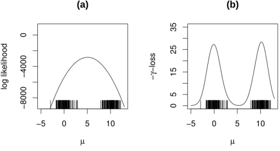
Here is a simple example that explains the motivation for employing the γ-divergence to capture the local structure. Consider the problem of estimating the Gaussian mean pa- rameterµ. The maximum likelihood estimator (MLE) of µ is given by the arithmetic mean of the data set as the unique maximum point of the log likelihood function. Similarly, theγ-estimator of µ is defined by the minimum point of the γ-loss function, which is the empirically estimated γ-divergence. It is known that the MLE behaves poorly in various situations where the Gaussianity assumption is inappropriate. For example, if the data are

(10)

derived from a mixture of two normal distributions while our model is normal, then the estimation with the log likelihood function fails, as shown in Figure 1 (a). This failure results from the unfaithfulness of the model. The estimation with the γ-loss function, however, captures all the components of the normal mixture, even though based on the unfaithful model. Figure 1 (b) shows that the γ-loss function has two local minimum points corresponding to the two mean values of the two normal distributions. That is, the two means can be estimated by the two local minimum points. This thesis applies such a property to detect local mean structure and local correlation structure in the data set, i.e. cluster analysis and parameter estimation of a copula model.

Cluster analysis is a common procedure for grouping similar objects in unsupervised learning (Jain et al., 1999; Xu and Wunsch, 2005; Hastie et al., 2009). The procedure stably produces a classification and is frequently used as a preprocessing technique before super- vised learning. Cluster analysis has wide applications over many disciplines in exploratory data analysis. See, for example, Jin et al. (2011) and Wu et al. (2011) for recent develop- ments. There are two main approaches in cluster analysis. One is the hierarchical approach, which describes a tree structure called a “dendrogram”. The other is the approach of data space partition, such as theK-means clustering. This thesis focuses on the latter approach from the point of view of statistical pattern recognition. We propose what we call the spontaneous clustering. It starts with finding cluster centers in a data set. For this purpose, we employ theγ-loss function of the Gaussian mean parameter. In the spontaneous clustering, we will propose to determine the cluster centers by the local minimum points of theγ-loss function. Almost all procedures via data space partition require to pre-determine the num-

(11)

ber of clusters; the selection of the number of clusters is a major challenge. A number of methods for this purpose have been proposed in the literature (Xu and Wunsch, 2005). Our clustering method can find the number of clusters automatically, as long as the value ofγ is properly fixed. The name “spontaneous clustering” comes from this property. Instead of the number of clusters, the value of the power indexγ should be determined. We will propose two methods to accomplish this aim. One is a heuristic choice ofγ that merely re- lies on the range of the data, and the other is a more sophisticated method based on Akaike Information Criterion (AIC).

The estimation of the Gaussian copula parameter is the other application of the local learning capability with the γ-divergence. Applications of copula models have been in- creasing in number in recent years. There are a variety of applications on finance, risk man- agement (McNeil et al., 2005), and multivariate time series analysis (Zhang et al., 2011). With copula models, the specification of the marginal distributions is parameterized separately from the dependence structure of the joint distribution. Hence it gives a convenient way of the construction of flexible and more general multivariate distributions. As far as we know, there exist only a few works that tackled with the identification and the statistical estimation of the mixture of copula models and most of them rely on MCMC algorithm. In this thesis we focus on a misspecified Gaussian copula model. In other words, a sample follows a distribution mixed with different sources but a statistical model we fit is just a single Gaussian copula. It is very hard to construct multivariate copulas for three or more random variables (Nelsen, 1999), while the Gaussian is an exception. So we start with the Gaussian copula model, but later in the section 4.3.6 we will show our method is closely related to

(12)

t-copula. As an example of misspecification, we consider that the underlying distribution is

τ cG(u; P1) + (1 − τ)c^G^{(u; P}²^), ^(1.1)

where τ is a mixing proportion and cG(u; P ) denotes the probability density function of the Gaussian copula with the correlation matrix parameterP . We see that the MLE for P almost surely converges toτ P1 _{+ (1 − τ)P}2 under the assumption (1.1), which means that the MLE fails to detect the structure of the underlying distribution. We make use of the γ-loss function of the Gaussian copula parameter for this problem. Our research shows that even if a single Gaussian copula model is incorrectly fitted to the data from the mixture distribution (1.1), theγ-loss function can detect both P1 ândP2separately ifP1 ândP2 âre

“distinct” enough andτ is close to 0.5. We, therefore, propose to use these local minimum points to detectP1 ^andP2^.

This thesis is organized as follows. In Chapter 2, we make a review of divergence measures and estimation with theγ-divergence. Chapter 3 describes the application of the γ-divergence to cluster analysis, where some existing clustering methods are also discussed. In Chapter 4, we provide a brief summary of copulas and discuss theγ-estimation for the Gaussian copula model. Summary and discussion are given in Chapter 5.

(13)

−5 0 5 10

−8000−40000

(a)

µ

log likelihood

−5 0 5 10

05152535

(b)

µ

−γ−loss

Figure 1.1: (a) Log likelihood function. (b) Minusγ-loss function Lγ(µ) (γ = 1). In (a) and (b), the data of size 200 is generated from the mixture of two standard normal distributions centered at 0 and 10, respectively.

(14)

Chapter 2 Minimum Divergence Estimation

2.1 Divergence Measures

In statistics, there are a number of indexes to measure the difference between two objects. Divergence measures reflect the difference between two probability distributions. They are defined by functionals which satisfy the following properties:

D(g, f ) ≥ 0 with equality if and only if g ≡ f, ^(2.1)

where g and f are probability density functions. Although a large number of divergence measures have been proposed in the literature, we present an introduction to two wide classes of divergence measures, Bregman divergence andU -divergence. The γ-divergence is derived from theβ-divergence, which is one of the U -divergence.

(15)

Bregman divergence

Bregman (1967) introduced a family of divergence measures in the following way,

Bψ(g, f ) =

∫

ψ(f (x)) − ψ(g(x)) − ψ^′(g(x))(f (x) − g(x))dx ^(2.2)

for any differentiable convex functionψ with ψ(0) = lim_t→0ψ(t) ∈ (−∞, ∞). Note that Bψ(g, f ) satisfies condition (2.1) due to the convexity of ψ (see Figure 2.1).

U -divergence

TheU -divergence is defined similar to the Bregman divergence (Murata et al. (2004)). Let U be a differentiable and strictly convex function. Then its derivative u = U^′is a monotonic function, which has the inverse functionξ = (u)⁻¹. TheU -divergence with respect to U is defined as

DU(g, f ) =

∫

U (ξ(f (x))) − U(ξ(g(x))) − U^′(ξ(g(x)))(ξ(f (x)) − ξ(g(x)))dx

=

∫

U (ξ(f (x))) − U(ξ(g(x))) − g(x)(ξ(f(x)) − ξ(g(x)))dx. ^(2.3)

We obtain theU -divergence by substituting ψ = U, g(x) = ξ(g(x)), and f (x) = ξ(f (x)) in (2.2). The advantage of the form (2.3) is allowing us to plug in the empirical distribution directly.

(16)

β-divergence

WhenU (t) = Uβ(t) = {1/(1 + β)}(1 + βt)^(1+β)/β (β > 0), the U -divergence becomes

DUβ^{(g, f ) =}

1 β

∫

{g(x)^β _{− f(x)}^β_{} g(x)dx −} ¹ 1 + β

∫

g(x)^1+β _{− f(x)}^1+βdx, (2.4)

which is called theβ-divergence (Basu et al., 1998; Minami and Eguchi, 2002).

γ-divergence

Theγ-divergence is derived from the β-divergence, which can lead more robust methods than theβ-divergence (Jones et al., 2001; Fujisawa and Eguchi, 2008). The γ-divergence is defined as

Dγ(g, f ) = −κ^γ

∫

g(x)f (x)^γdx + (∫

g(x)^1+γdx )_1+γ¹

, (2.5)

whereκ_γ =(∫ f(x)^1+γdx⁾^−γ/(1+γ).

The derivation of the γ-divergence is as follows. Consider the following optimization problem,argmin

v>0

DUβ(g, vf ). The first derivative of DUβ(g, vf ) with respect to v becomes

d

dv^D^U^β(g, vf ) = −v^β−1

∫

f (x)^βg(x)dx + v^β

∫

f (x)^1+βdx.

Set the derivative to 0. Then we have

minv>0 ^D^U^β^{(g, vf ) =}

1 β(1 + β)

(∫

g(x)^1+β_{dx −} ^{(∫ f(x)}

β_g(x)dx)1+β

(∫ f(x)^1+βdx)^β )

. (2.6)

(17)

The logarithmic of the ratio of the first and second terms of (2.6) is equal to

1

β(1 + β)^log

(∫ g(x)^1+βdx)(∫ f(x)^1+βdx)^β (∫ f(x)^βg(x)dx)^1+β

= ¹

β {

− log

∫ g(x)f (x)^βdx

(∫ f(x)^1+β)^β/(1+β) ^{+ log} (∫

g(x)^1+βdx

)1/(1+β)^}

.

Then we consider the value

−_{(∫ f(x)}_1+β¹

)^β/(1+β)

∫

g(x)f (x)^βdx + (∫

g(x)^1+βdx

)1/(1+β)

,

which corresponds toDγ(g, f ) if β = γ. Note that Dγ(g, f ) satisfies condition (2.1) from this derivation.

2.2 γ-Estimation

Suppose a random sample is generated from a population distribution with density function g. Let {f(·, θ)} be a family of density functions indexed by parameter θ. The γ-cross entropy betweeng and f (·, θ) is defined as

Cγ(g, f (·, θ)) = −κ^γ^(θ)

∫

g(x)f (x, θ)^γdx,

with power indexγ > 0, where κγ(θ) is the normalizing constant defined as

κγ(θ) = (∫

f (x, θ)^1+γdx )₋_1+γ^γ

.

(18)

The Boltzmann-Shannon cross entropy betweeng and f (·, θ) is defined by

−

∫

g(x) log f (x, θ)dx.

Theγ-cross entropy and the Boltzmann-Shannon cross entropy have the following relation sinceκγ(θ) converges to 1 if γ tends to 0.

γ→0lim

C_γ(g, f (·, θ)) + 1

γ ^{= −}

∫

g(x) lim

γ→0

( f (x, θ)^γ_{− 1} γ

) dx

= −

∫

g(x) log f (x, θ)dx.

Hence the Boltzmann-Shannon cross entropy can be seen as the0-cross entropy, and the γ-cross entropy can be regarded as an extension of the Boltzmann-Shannon cross entropy. Theγ-entropy of g is defined as Hγ(g) = Cγ(g, g). Then the γ-divergence between g and f (·, θ) becomes

Dγ(g, f (·, θ)) = C^γ(g, f (·, θ)) − H^γ^(g).

Recall that theγ-divergence Dγ(g, f (·, θ)) is nonnegative, and D^γ(g, f (·, θ)) is equal to 0 if and only ifθ satisfies that g(x) = f (x, θ) almost everywhere x. From these properties, Dγ(g, f (·, θ)) can be seen as a kind of distance between g and f(·, θ) although it does not satisfy the symmetry. When our aim is to find the closest distribution to g in model {f(·, θ)} with respect to the γ-divergence, we only have to find the global minimum point ofDγ(g, f (·, θ)) with respect to θ, which is equal to that of C^γ(g, f (·, θ)).

(19)

The γ-loss function is defined by an estimator of the γ-cross entropy. Let {x¹^{, x}²^, . . . , xn} be a random sample generated from a population distribution with density function g and {f(·, θ)} be our statistical model. The γ-loss function for f(·, θ) associated with the γ-divergence is given by

Lγ_{(θ) = −κ}γ(θ)¹ n

n

∑

i=1

f (xi, θ)^γ.

We extend the definition of the γ-cross entropy to any distributions. For any distribution functionG, the γ-cross entropy between G and f (·, θ) is defined as

C_γ(G, f (, θ)) = −κγ^(θ)

∫

f (x, θ)^γdG(x).

Note that Lγ(θ) is equal to Cγ( ˆG, f (·, θ)) with empirical distribution function ˆ^{G, so that} E(Lγ(θ)) = Cγ(g, f (·, θ)), and L^γ(θ) almost surely converges to Cγ(g, f (·, θ)). The γ- estimator ofθ is defined by the global minimum point of L_γ(θ) (Eguchi and Kato, 2010). From the definition of theγ-estimator, it satisfies Fisher consistency. If the density function g belongs to the statistical model {f(·, θ)}, then the γ-estimator satisfies asymptotic consistency and normality. Theγ-loss function and the log likelihood function satisfy the following relation

γ→0lim

Lγ(θ) + 1

γ ^{= −}

1 n

n

∑

i=1

log f (xi, θ).

Hence the MLE can be regarded as the 0-estimator and the γ-estimator can be seen as an

(20)

extension of the MLE.

(21)

Figure 2.1: Illustration of the Bregman divergence.

(22)

Chapter 3 Cluster Analysis

3.1 Existing Methods

In this section, we make a review of three clustering algorithms, theK-means, model-based, and mean shift clustering. The model-based clustering is based on some parametric models while theK-means clustering considers the Euclidean distance among the data points. In the mean shift clustering, density estimates are used for finding cluster centers.

3.1.1 K-Means Clustering

TheK-means clustering is to minimize the lack of homogeneity of each cluster based on the Euclidean distance. For the K-means algorithm, the number of clusters K has been fixed by the investigator.

Let _{x₁, x₂, . . . , x_n} be a data set, and K be the number of clusters. The dispersion

(23)

matrix based on the data set is defined as

TK =

K

∑

k=1

∑

x∈Ck

(x − ¯x)(x − ¯x)^⊤^,

whereCk ^{is the} kth cluster, and ¯x = (1/n)^∑ⁿ_i=1xi. The dispersion matrix represents the total dispersion, and it can be decomposed into two matrices, the with-in cluster dispersion matrixWK and the between-cluster dispersion matrixBK^,

WK =

K

∑

k=1

∑

x∈Ck

(x − ¯x^k)(x − ¯x^k⁾^⊤^{, B}^K ⁼

K

∑

k=1

nk(¯xk_{− ¯x)(¯x}k_{− ¯x)}^⊤,

so thatTK = WK+BK^{, where}nkis the number of objects inCk^{, and}x¯k = (1/nk)^∑_x∈C_kx. For cluster analysis, there are a lot of criteria based onW_K andB_K, for example, minimization ofdet(WK), and maximization of tr(BKW_K⁻¹) (see Everitt et al. (2011) for more detailed discussion). The criterion for the K-means algorithm is minimization of tr(WK). This criterion is equivalent to minimization of the lack of homogeneity of clusters, that is,

tr(WK) =

K

∑

k=1

1 2nk

∑

x,x^′_∈Ck

∥x − x^′∥²^.

In practice, the investigators will have to estimate the number of clusters in the data set. It is of great importance to select the number of clusters, because the clustering results may change drastically as the number of clusters increases. Two criteria will be shown for selection of the number of clusters for theK-means clustering.

(24)

CH

In Cali´nski and Harabasz (1974), a criterion CH(k) is defined by

CH(k) = ^tr(B^k^{)/(k − 1)} tr(W_k_{)/(n − k)}^.

This criterion is analogous to theF -statistic for analysis of variance in the univariate case. They propose to select the number of clustersk, which maximizes CH(k).

Gap Statistic

The within-cluster sum of squares tr(Wk) monotonically decreases as k increases, but there existsk^∗ such that for_{k ≥ k}^∗, tr(Wk) decreases smaller than for k < k^∗. Such ak^∗ is used as an optimal value for the number of clusters. In Tibshirani et al. (2001), they provide a more sophisticated procedure to formulate this heuristic.

The gap statistic is defined by

Gap_n(k) = E_n^∗(log(tr(Wk))) − log(tr(W^k^)),

where E_n^∗ denotes the expectation under a sample size n from a reference distribution. They propose the optimal value of k, which maximizes the gap statistic with taking the sampling distribution into account. Then E_n^∗(log(tr(Wk))) is calculated by a Monte Carlo approximation. In practice, the selected number of clusters is the smallestk such that

Gap(k) ≥ Gap(k + 1) − s^k+1^,

(25)

wheresk+1 is a standard error.

3.1.2 Model-Based Clustering

A model-based clustering is to postulate a mixture density function for the population distribution, from which the data are sampled. Then the parameters in the mixture density function are estimated, and the posterior probabilities are calculated by plugging-in the estimators for the counterparts in the mixture densities. Each object is assigned to the cluster which maximizes the estimated posterior probability that the object is in the cluster.

Letfk(x, θk) be a density function parametrized by θk^{, and}g(x, τ, θ) be a mixture density function,

g(x, τ, θ) =

K

∑

k=1

τ_kf_k(x, θ_k),

whereτ = (τ1, τ2, . . . , τK)^⊤andθ = (θ₁^⊤, θ₂^⊤, . . . , θ^⊤_K)^⊤. Hereτ1, τ2, . . . , τKare the mixing proportions, that is, they are nonnegative and satisfy that^∑^K_k=1τ_k = 1. The model-based clustering postulatesg(x, τ, θ) for the population distribution, and we estimate the parame- terτ and θ.

Although there are a lot of estimation methods, we focus on the maximum likelihood estimation. Since the log likelihood function for g(x, τ, θ) is often very complicated, it is hard to calculate the maximum likelihood estimator (MLE) by using the log likelihood forg(x, τ, θ). An alternative to obtain the MLE is the EM-algorithm (see Dempster et al. (1977)). From this, we focus on the situation where the component densities of the mixture density are normal. Letϕ(x, µ, Σ) be the density function of the normal distribution with mean vectorµ and covariance matrix Σ. We postulate ϕ(x, µ_k, Σ_k) as the kth component

(26)

density of the mixture density function. Then the EM-algorithm for normal mixture is given as follows.

EM-algorithm for normal mixture

Step 1 Set appropriateτ₁⁽⁰⁾, τ₂⁽⁰⁾, . . . , τ_K⁽⁰⁾, µ⁽⁰⁾₁ , µ⁽⁰⁾₂ , . . . , µ⁽⁰⁾_K , Σ⁽⁰⁾₁ , Σ⁽⁰⁾₂ , . . . , Σ⁽⁰⁾_K .

Step 2 Givenτ₁^(t), . . . , Σ^(t)_K, calculateτ₁^(t+1), . . . , Σ^(t+1)_K by the following update formula.

τ_k^(t+1) = ¹ n

n

∑

i=1

τ_ki^(t),

τ_ki^(t) = ^τ

(t)

k ^ϕ(xⁱ^{, µ} (t) k ^{, Σ}

(t) k ⁾

∑K j=1^τ

(t)

j ^ϕ(xⁱ^{, µ} (t) j ^{, Σ}

(t) j ⁾

,

µ^(t+1)_k =

n

∑

i=1

τ_ki^(t)

∑n j=1^τ

(t) kj

x_i,

Σ^(t+1)_k =

n

∑

i=1

τ_ki^(t)

∑n j=1^τ

(t) kj

(x_i_{− µ}^(t+1)_k )(x_i_{− µ}^(t+1)_k )^⊤.

Step 3 Repeat Step 2 until all parameters converge.

For selection ofK, we can use information criteria, such as AIC and BIC,

AIC _{= −2}

n

∑

i=1

log f (xi, ˆθ, ˆτ ) + 2(number of parameters),

BIC _{= −2}

n

∑

i=1

log f (x_i, ˆθ, ˆτ ) + log(n)(number of parameters),

and selectk minimizing those criteria.

(27)

3.1.3 Mean Shift Clustering

A mean shift clustering (MSC) with the Gaussian kernel is to determine the cluster centers by the modes of the density estimate defined by

fˆh(x) = ¹ nh^p

n

∑

i=1

exp₍₋_2h¹2_{∥x − x}i_∥²

)

(2π)^p/2 ^. ^(3.1)

We supposex^(m)_i is the position ofxi ^{at stage}m of the procedure, where x⁽⁰⁾_i = xi^{. Then}

x^(m)_i is updated by

x^(m+1)_i =

n

∑

j=1

exp⁽_−∥x^(m)_i _{− x}j_∥²/(2h²)⁾

∑n ℓ=1^exp

(−∥x^(m)i − x^ℓ∥²^/(2h²⁾^{) x}^j .

Note that eachx^(m)_i will converge to a mode of the density estimate defined by (3.1). The set_{x^(m)_i : m ∈ N} is called the trajectory of xi^{. Let}{x1^(∞), . . . , x^(∞)n _{} be {c}1, . . . , c_K_h_}. Then we defineck as the cluster center, and eachxi is assigned to the cluster of which the centerckis equal tox^(∞)_i .

For MSC, a bandwidth selection by Einbeck (2011) can be used. Suppose c_i,h is the cluster center to whichxi is assigned. The self-coverage for cluster analysis is defined as

S(h) = ¹ n

n

∑

i=1

1(∥xⁱ − c^i,h∥ ≤ h),

where1(·) is the indicator function. Assume we have evaluated S(h) over a grid of band-

(28)

widthsh1 < · · · < h^L. The curvature ofS(h) is approximated by

△²^S(h^ℓ^{) = S(h}^ℓ+1) − 2S(h^ℓ^{) + S(h}ℓ−1^).

Let h(j) be the bandwidth yielding the jth lowest of △²^S(h^ℓ), h = 1, . . . , L, under the constraint

S(hℓ) > max{S(h¹), . . . , S(h_ℓ−1_{), s},}

wheres ∈ (0, 1) is a pre-determined constant. A value of s = 1/3 is recommended (Ein- beck, 2011). Thenh(1) is used as the optimal value.

3.2 Spontaneous Clustering

This section is based on the paper (Notsu et al., 2014). We begin with reconsidering the motivational example in the introduction from the point of view of cluster analysis. First, we consider a trivial situation, where the number of clusters is one. For example, assume thatx1, . . . , xn ^{in R}^p follow a normal distribution with the mean vectorµ and the identity covariance matrix. Then the log likelihood function multiplied by−1/n is given by

L0_{(µ) = −}

1 n

n

∑

i=1

log

(exp₍₋¹₂_∥xi_{− µ∥}²

) (2π)^p/2

) ,

which is equal to 1/(2n)(^∑ⁿ_i=1_∥x_i _{− µ∥}² + p log 2π), where ∥ · ∥ denotes the Euclidean norm. The MLE ofµ is just the sample mean, by which the cluster center can be determined. However, if there is more than one cluster, then the MLE does not work. We take another

(29)

estimator ofµ, the γ-estimator (Eguchi and Kato, 2010). In general, for a location family {f(x − µ) : µ ∈ R^p}, where f(x) is a probability density function, the γ-loss function is defined as

L_γ,f_{(µ) = −}¹ n^κ^γ

n

∑

i=1

f (x_i_{− µ)}^γ, (3.2)

whereκγ =(∫ f(x)^1+γdx⁾⁻

γ

1+γ_{. If}f (x) is the normal density function with mean vector 0 and the identity covariance matrix, then the γ-loss function becomes

Lγ_{(µ) = −}

1

n{(1 + γ)(2π)^γ}^2(1+γ)^γp

n

∑

i=1

(exp₍₋¹₂_∥xi_{− µ∥}²

) (2π)^p/2

)γ

, (3.3)

where the subscriptf is omitted for simplicity. The γ-estimator of the normal mean µ is the value which minimizesLγ(µ).

We consider a standard situation ofK clusters, where the density function of the population distribution hasK modes, for example,

g(x) =

K

∑

k=1

τkfk(x),

K

∑

k=1

τk = 1, τk > 0, k = 1, . . . , K, (3.4)

wherefk(x) is a unimodal density function. As stated above, the MLE does not work in this situation. It is expected that the γ-loss function Lγ(µ) has K local minimum points corresponding toK mean vectors with respect to f₁, . . . , f_K. Figure 1 (b) shows thatL_γ(µ) has two local minimum points when the data have two clusters. Thus the cluster centers defined by the local minimum points lead to a clustering method similar to theK-means

(30)

clustering.

The proposed procedure appears to be similar to density-based clustering methods, for example, the mean shift clustering (Cheng, 1995), since theγ-loss function Lγ(µ) resem- bles the kernel density estimate with the Gaussian kernel (3.1). Ifµ = x, and h² = γ⁻¹, thenLγ(µ) and ˆfh(x) are essentially the same, apart from a constant. Since the mean shift clustering defines the cluster centers by modes of the density estimate (3.1), the proposed procedure is the same with the mean shift clustering, that is, finding modes of equation (3.3).

There are some differences between them, however. We employ the γ-loss function, not density estimates, so that we will naturally estimate covariance structures of clusters by incorporating the γ-loss function for the covariance matrix of the normal distribution. In addition, we will propose the selection for the power index γ based on the theory of theγ-loss function, which also gives a new insight or different view to the selection of the bandwidthh for the density estimation. Lγ(µ) is a loss function for the normal mean µ; fˆh(x) is a density estimate obtained by smoothing the histogram in terms of the Gaussian kernel function. In general, kernel density estimates are given by

1 nh^p

n

∑

i=1

W^{( x − x}ⁱ h

)

, (3.5)

where W is a kernel function. Two equations (3.2) and (3.5) are quite different forms derived from different ideas.

(31)

3.2.1 γ-Loss Function for the Normal Distribution

We consider theγ-loss function for the normal distribution with the mean vector µ and the covariance matrixΣ,

Lγ(µ, Σ) = − det Σ⁻^2(1+γ)^γ

n

∑

i=1

exp⁽₋^γ

2^(xⁱ^{− µ)}

⊤_Σ−1_(x i_{− µ)}

)

, (3.6)

apart from a constant. In the remainder of the thesis, we omit a constant term that does not affect the optimization. An iteration algorithm to find the local minimum points of L_γ(µ, Σ) has been proposed in Fujisawa and Eguchi (2008) and Eguchi and Kato (2010). It is obtained by differentiatingLγ(µ, Σ) with respect to µ and Σ⁻¹and setting the derivatives to0. The algorithm is a concave-convex procedure (CCCP) (Yuille and Rangarajan, 2003), so that it is guaranteed to decrease theγ-loss function monotonically as the iteration step t increases. It is described below.

Step 1 Set appropriateµ0 ^andΣ0as initial values.

Step 2 Givenµt^andΣt, calculateµt+1^andΣt+1by the following update formulas,

µt+1 =

n

∑

i=1

wγ(xi, µt, Σt)xi, (3.7)

Σt+1 = (1 + γ)

n

∑

i=1

wγ(xi, µt, Σt)(xi_{− µ}t+1)(xi_{− µ}t+1)^⊤, (3.8)

where

w_γ(x, µ, Σ) = ^exp⁽⁻

γ

2^{(x − µ)}^⊤^Σ⁻¹^{(x − µ)}

)

∑n

j=1^exp(−^γ2^(x^j− µ)^⊤^Σ⁻¹^(x^j− µ)^{) .}

(32)

Step 3 For a sufficiently small numberε, repeat Step 2 while

∥µ^t+1− µ^t∥ + ∥Σ^t+1− Σ^t∥^F^{> ε,}

where_{∥ · ∥}_Fdenotes the Frobenius norm.

Ifγ = 0, then the right hand sides of equations (3.7) and (3.8) are equal to the sample mean vector and covariance matrix, respectively, which are just the MLEs. If our aim is to obtain the local minimum points of Lγ(µ), then we only have to update µt ^{and fix} Σt ^{to be the}

identity matrixI. Similarly, if our aim is to obtain the local minimum points of Lγ(µ, Σ) with fixedµ, then we only have to update Σt^{and fix}µt = µ.

3.2.2 Spontaneous Clustering Algorithm

In general, the spontaneous clustering based on a density functionf (x, θ) with parameter θ is defined as follows.

Spontaneous Clustering

Step 1 Find the local minimum points ofLγ(θ), denoted by ˆθ1, . . . , ˆθK^{, where}Lγ(θ) is the γ-loss function for f (x, θ).

Step 2 ConsiderK clusters according to ˆθ₁, . . . , ˆθ_K, and assign the data to the clusters.

As a special case, the spontaneous clustering based on the normal distribution is defined as follows. We set Θµ ^and Θ(µ,Σ) to be the empty sets at the start of the algorithm. The algorithm of section 3.2.1 is employed in the spontaneous clustering below.

(33)

Spontaneous Clustering Based on the Normal Distribution

Step 1-1 If Θµ is the empty set, choose M initial values x(1), . . . , x(M ) in the data set {x¹, . . . , xn} at random. Otherwise, choose initial values in {x¹, . . . , xn} as follows: x₍₁₎, . . . , x_{(M )} areM maximum points of d(·, Θµ^{), where}

d(x, Θµ) = min

µ∈Θˆ µ^{∥x − ˆµ∥.}

Step 1-2 Apply the algorithm in section 3.2.1 to the data set M times with each initial value x(i), i = 1, . . . , M to find the local minimum points of Lγ(µ). Then add the obtained local minimum points toΘµ^.

Step 1-3 Repeat Step 1-1 and 1-2 until the number of elements inΘµdoes not increase.

Step 1-4 For each local minimum point_{µ ∈ Θ}ˆ µ, obtain a minimum point ofLγ(ˆµ, Σ) with respect toΣ, denoted by ˆΣ, with the algorithm in section 3.2.1. Then add (ˆµ, ˆΣ) to Θ_(µ,Σ).

Step 2 WriteΘ(µ,Σ)^by_{(ˆµk, ˆΣk_)}^K_k=1and assign each observationxi^{to the ˆ}kth cluster with

k = argminˆ

k=1,...,K

(xi_{− ˆµ}k)^⊤Σ^ˆ⁻¹_k (xi_{− ˆµ}k).

The centers and the covariance matrices of clusters are defined as(ˆµ_k, ˆΣ_k). In the remainder of this chapter, we focus on the spontaneous clustering based on the normal distribution.

(34)

3.2.3 Selection Procedure for _γ

The value of the power index γ plays a key role in the spontaneous clustering, because γ affects the number of clusters obtained by the spontaneous clustering. We propose two methods to select the value ofγ. One is a heuristic choice of γ that depends on the range of the data. Our proposal isγ = 72/Rˆ ², whereR is defined by the maximum range:

R = max

j=1,...,p

{(

i=1,...,nmax ^x^ij )

− (

i=1,...,nmin ^x^ij )}

,

wherex_i = (x_i1, . . . , x_ip)^⊤. The outline of the derivation ofγ is as follows. Suppose theˆ data set is generated from the mixture of two normal distributions centered at µ1 ^and µ2

with the identity covariance matrix and the equal mixing proportions, respectively. Our simulation result suggests that if_∥(µ₁_{− µ}₂_{)/2∥ = 3}^√2/2= 2.12, then the value of γ needs^. to be greater than or equal to 1 for two local minimum points ofLγ(µ) to exist. Proposition 3.2.1 states that if all the data are multiplied by a scalara, and the spontaneous clustering is applied to the transformed data, then the value ofγ needs to be greater than or equal to a⁻² to guarantee the existence of two local minimum points of Lγ(µ). If ∥(µ¹ − µ²)/2∥ = r, thena = r/(3^√2/2). Hence we propose to use the value of γ defined as

ˆ γ =

( r

3^√2 2

)₋₂

= ⁹

2r²^. ^(3.9)

The value ofr can be estimated by the range of the data. Let R_j be the range of the jth variable. If there are K disjoint clusters lying side by side on a line parallel to the axis of thejth variable, then we can estimate r by Rj/(2K) as shown in Figure 3.1. There are p

(35)

variables, sop directions have to be considered simultaneously. We use the maximum range R and estimate r by R/(2K). The value of K can be determined from our prior knowledge about the possible number of clusters. IfK = 2, we have ˆγ = 72/R². We observe that this rule works well in several empirical studies, although a complete theoretical background is missing.

We also propose a more sophisticated method based on AIC. The value ofγ which minimizes AIC is recommended as the optimal selection ofγ. Let Kγbe the number of clusters and(ˆµγk, ˆΣγk), k = 1, . . . , Kγbe the centers and the covariance matrices of clusters resulting from the spontaneous clustering. Letϕ(x, µ, Σ) be the density function of the normal distribution with the mean vectorµ and the covariance matrix Σ. Then ϕ(x, ˆµγk, ˆΣγk) serves as a density estimator of the mixture componentfk(x) in (3.4). The result of the spontaneous clustering implies the mixture of normal distributions as an estimator of the density function of the population distributiong in (3.4),

ˆ gγ(x) =

Kγ

∑

k=1

ˆ

τγkϕ(x, ˆµγk, ˆΣγk),

where τˆγk is an estimator of the mixing proportion τk defined as the proportion of the observations assigned to thekth cluster. The AIC based on ˆgγis defined as follows.

AIC_γ _{= −2}

n

∑

i=1

log ˆgγ(xi) + 2 {

Kγ

p(p + 3)

2 ^{+ K}^γ^{− 1} }

.

We claim that the value ofγ that minimizes AICγ is the optimal one.

(36)

3.2.4 Behavior of the γ-Loss Function

We provide a justification for the spontaneous clustering by exploring its theoretical aspects. The key fact is that the γ-loss function Lγ(µ) has K local minimum points if the data set consists ofK cluster groups.

The Existence of Local Minimum Points

In this section, we consider the conditions for the existence of local minimum points of Lγ(µ). As we discussed in section 3.2.2, the cluster centers are defined at the local minimum points ofLγ(µ), so it is important to know when the γ-loss function has local minimum points.

To simplify the argument, we assume that the data set is generated from the mixture of two normal distributions with the covariance matrixσ²I,

g(x) = τ1ϕ(x, µ1, σ²I) + τ2ϕ(x, µ2, σ²I), τ1+ τ2 = 1, τk > 0, k = 1, 2.

For ease of calculation, we consider n = ∞. As n tends to ∞, L^γ(µ) almost surely converges to theγ-cross entropy defined by

Cγ(g, ϕ(·, µ, I)) = −κ^γ

∫

g(x)ϕ(x, µ, I)^γdx, (3.10)

where κ_γ = (∫ ϕ(x, 0, I)^1+γdx⁾⁻^1+γ^γ . Section 2.2 contains a general introduction to the

(37)

γ-cross entropy. Then Cγ(g, ϕ(·, µ, I)) becomes

Cγ(g, ϕ(·, µ, I)) = ^∑

k=1,2

τkCγ_{(ϕ(·, µ}k, σ²I), ϕ(·, µ, I))

∝ − ^∑

k=1,2

τkϕ (

µ, µk, (

σ²+ ¹ γ

) I

) ,

which is just minus the density function of the mixture of two normal distributions with the same covariance matrix(σ²+ 1/γ)I. Hence, the local minimum points of Cγ(g, ϕ(·, µ, I)) are equal to the modes of the density function of the normal mixture. Figure 3.2 shows

−C^γ(g, ϕ(·, µ, I)) with dimension p = 2, where −C^γ(g, ϕ(·, µ, I)) has one or two modes depending on the values ofµ1, µ2, τ1, τ2^{, and}γ. For the univariate case, a necessary and sufficient condition that the density function of the mixture of two normal distributions should be bimodal is given in de Helguero (1904). We use a similar technique as in de Helguero (1904) to obtain a necessary and sufficient condition forCγ(g, ϕ(·, µ, I)) to have two local minimum points.

Proposition 3.2.1 Letν = (µ1_{− µ}2)/2 and d = ∥ν∥²− (σ²+ 1/γ). Then Cγ(g, ϕ(·, µ, I)) has two local minimum points if and only if the following three conditions hold:

d > 0, (3.11)

exp

( 2γ

1 + γσ²^∥ν∥

√d )

> ^γ 1 + γσ²

(

∥ν∥ +^√^d⁾²^τ_τ¹

2

, (3.12)

exp (

− ^2γ

1 + γσ²^∥ν∥

√d )

< ^γ 1 + γσ²

(∥ν∥ −^√^d⁾² ^τ¹ τ2

. (3.13)

In particular, if τ1 = τ2, then (3.12) and (3.13) hold for any d > 0. When the two local

(38)

minimum points exist, they lie on the segment betweenµ1 ^andµ2. The one closer toµ1 ^and

the other closer toµ2are denoted byµ^∗₁andµ^∗₂, respectively. Then_∥µ₁_−µ^∗₁_{∥ and ∥µ}₂_−µ^∗₂_∥ are bounded above by

∥ν∥ −

√

∥ν∥²− (

σ²+ ¹ γ

) .

Proof. No generality is lost by assumingµ2 _{= −µ}1. The gradient ofCγ(g, ϕ(·, µ, I)) is given by

∂Cγ(g, ϕ(·, µ, I))

∂µ ^{∝ τ}¹^{ϕ(µ, µ}¹^{, (σ}

2+ 1/γ)I)(µ − µ¹⁾

+τ2_{ϕ(µ, −µ}1, (σ²+ 1/γ)I)(µ + µ1). (3.14)

From (3.14), every local minimum point of Cγ(g, ϕ(·, µ, I)) should exist on the segment between_−µ₁andµ1. The Hessian matrix ofCγ(g, ϕ(·, µ, I)) is given by

∂²Cγ(g, ϕ(·, µ, I))

∂µ∂µ^⊤ ^{∝ −τ}¹^{ϕ(µ, µ}¹^{, (σ}

2_{+ 1/γ)I)} ^γ

1 + σ²γ^{(µ − µ}¹^{)(µ − µ}¹⁾

⊤

−τ²ϕ(µ, −µ¹^{, (σ}²^{+ 1/γ)I)}_{1 + σ}^γ ₂_γ^{(µ + µ}¹^{)(µ + µ}¹⁾^⊤ +τ₁ϕ(µ, µ₁, (σ² + 1/γ)I)I

+τ2_{ϕ(µ, −µ}1, (σ² + 1/γ)I)I. (3.15)

Letµ(t) = tµ₁. From (3.15),µ(t) is a local minimum point of C_γ(g, ϕ(·, µ, I)) if and only if t is a local minimum point of Cγ(g, ϕ(·, µ(t), I)) with respect to t. C^γ(g, ϕ(·, µ(t), I))

(39)

becomes

Cγ(g, ϕ(·, µ(t), I)) ∝ −τ¹exp(−C(t − 1)²) − τ²exp(−C(t + 1)²^),

whereC is equal to ∥µ¹∥²^{γ/(2(1 + σ}²γ)). The derivative of Cγ(g, ϕ(·, µ(t), I)) is given by

d

dt^C^γ(g, ϕ(·, µ(t), I)) ∝ τ¹exp(−C(t − 1)²)(t − 1) + τ²exp(−C(t + 1)²^{)(t + 1).}

It is possible to restrict−1 < t < 1. Then

d

dt^C^γ(g, ϕ(·, µ(t), I)) > 0

⇐⇒ exp(−C(t + 1)²+ C(t − 1)²^{) >} ^{(1 − t)τ}¹ (t + 1)τ2

⇐⇒ −4Ct + log(t + 1) − log(1 − t) − log^τ_τ¹

2

> 0. (3.16)

Leth(t) be the left hand side of inequality (3.16). The derivative of h(t) is given by

h^′(t) = −4C +_{t + 1}¹ ⁺ ¹ 1 − t^,

and

h^′(t) > 0 ⇐⇒ −4C(1 − t²) + (1 − t) + (1 + t) > 0

⇐⇒ t²− (

1 −_2C¹ )

> 0.

If1 − 1/(2C) ≤ 0, then h^′(t) ≥ 0, and C^γ(g, ϕ(·, µ(t), I)) has one local minimum point.

(40)

HenceCγ(g, ϕ(·, µ(t), I)) has two local minimum points if and only if

1 −_2C¹ > 0, h(−D) > 0, h(D) < 0,

whereD is the positive solution of equation h^′(t) = 0, that is D =√1 − 1/(2C). Condi- tion1 − 1/(2C) > 0 is equivalent to ∥µ¹∥²− (σ² + 1/γ) > 0. Condition h(−D) > 0 is equivalent to

exp

( 2γ

1 + σ²γ^∥µ¹^∥

√

∥µ¹∥²− (

σ²+ ¹ γ

)⁾

> ^γ 1 + σ²γ

(

∥µ¹∥ +

√

∥µ¹∥²− (

σ² + ¹ γ

)⁾² τ1

τ2

,

and conditionh(D) < 0 is equivalent to

exp (

− ^2γ

1 + σ²γ^∥µ¹^∥

√

∥µ1∥² − (

σ²+ ¹ γ

)⁾

< ^γ 1 + σ²γ

(

∥µ¹∥ −

√

∥µ¹∥²− (

σ²+ ¹ γ

)⁾² τ₁ τ2

.

Note thatµ^∗₁ is on the line between Dµ1 ^andµ1. Similarly _(−µ₁)^∗ is on the line between

−µ¹ ^and−Dµ¹^{. Then}

∥µ^∗1− µ¹∥ ≤ (1 − D)∥µ¹∥ = ∥µ¹∥ −

√

∥µ¹∥²− (

σ²+ ¹ γ

) .

Ifτ₁ = τ₂, thenh(±1) = ±∞, h(0) = 0. Condition 1 − 1/(2C) > 0 is equivalent to h^′(0) < 0. Hence two conditions h(−D) > 0, h(D) < 0 hold whenever 1 − 1/(2C) > 0

(41)

holds. _✷ Ifµ1 ^andµ2 are distinct enough, then conditions (3.11), (3.12), and (3.13) hold. Con- dition (3.11) means that the distance betweenµ1 ^and µ2 should be large for the existence of two local minimum points; condition (3.12) and (3.13) mean that if τ1 _{̸= τ}2^{, then the}

distance betweenµ1 ^andµ2 should be larger compared to the case whenτ1 = τ2^.

By proposition 3.2.1, for any σ², if µ1 ^and µ2 are distinct enough, then there exists γ that guarantees the existence of two local minimum points of Cγ(g, ϕ(·, µ, I)), and two clusters are defined at the same instant. In addition, although the center of a clusterµ^∗_kdoes not coincide with the normal meanµk (k = 1, 2), it becomes arbitrarily close to µk^{, when}

∥µ¹ − µ²∥ becomes large.

3.2.5 Comparison among Spontaneous Clustering and Existing Meth-

ods

In this section, we clarify the differences among the three clustering methods, the spontaneous clustering based on the normal distribution, the mean shift clustering with the Gaus- sian kernel, and theK-means clustering. For a given number of clusters K, the K-means clustering determines the cluster centersc1, . . . , cK ^by

argmin

c1,...,cK∈R^p n

∑

i=1

k∈{1,...,K}min ^∥xⁱ^{− c}^k^∥

2_. _(3.17)

Eachxi is assigned to the cluster of which the centerck is the nearest toxi in terms of the Euclidean distance.

(42)

To find the cluster centers, the spontaneous clustering and the mean shift clustering use the modes of the same function sinceLγ(µ) and ˆfh are essentially the same apart from a constant. On the other hand, the K-means clustering uses the minimum point defined by (3.17). After determining the cluster centers, to assign the data to clusters, theK-means clustering uses the Euclidean distance, but the spontaneous clustering uses the Mahalanobis distance. The mean shift clustering employs the mean shift trajectories for assignment. Table 3.1 summarizes the comparison among the three clustering methods.

3.3 Simulation and Data Analysis

3.3.1 Simulation 1: The Case of Spherical Clusters

We demonstrate the performance of the spontaneous clustering (SC) in comparison with the K-means clustering and the mean shift clustering (MSC). In this simulation, we suppose that the covariance matrices of clusters are known to be the identity matrix. Hence, in SC, the covariance matrices of clusters were not estimated and fixed to be the identity matrix. The performance of clustering is measured by BHI as defined below.

The value of γ for SC was determined by the range of data (R) and AIC described in section 3.2.3 and a heuristic bandwidth selection (HBS) in kernel density estimation. The value selected by HBS is given by

ˆ

γ =^{( n(p + 2)} 4

)_p+4² /ˆσ²,

(43)

whereσˆ² is the average of sample variances for each variable (see Silverman (1986) page 87). For theK-means clustering, the method by Cali´nski and Harabasz (1974) and the gap statistic by Tibshirani et al. (2001) were used to fix the number of clusters.

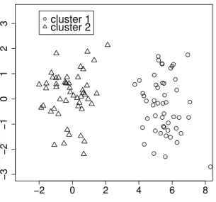
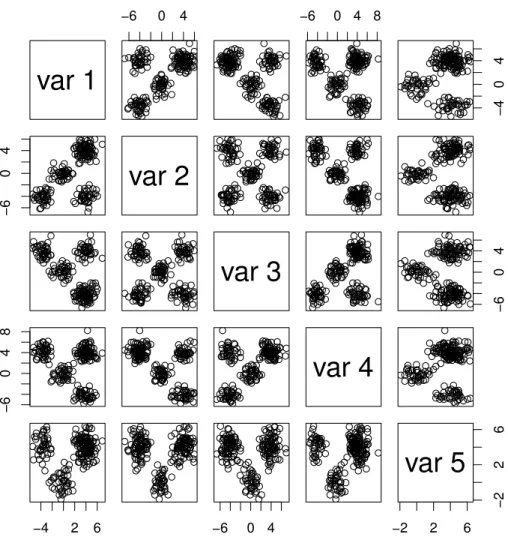
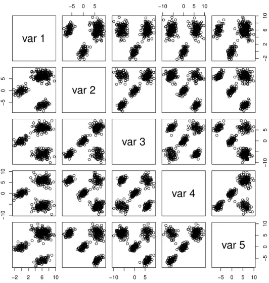
We considered four different simulation settings with the sample size 200. The samples were generated from the mixture of five standard normal distributions with

(a) the mean vectors(0, 0, 0, 0, 0)^⊤, (4, 4, 4, 4, 4)^⊤, (−4, −4, 4, 4, 4)^⊤^, (4, −4, −4, 4, 4)^⊤^{, and}(4, 4, −4, −4, 4)^⊤, and equal mixing proportions;

(b) the same mean vectors as (a) but different mixing proportions 0.025, 0.025, 0.375, 0.375, and 0.2;

(c) the mean vectors(0, 0, 0, 0, 0, 0, 0, 0, 0, 0)^⊤, (4, 4, 4, 4, 4, 4, 4, 4, 4, 4)^⊤, (−4, −4, −4, 4, 4, 4, 4, 4, 4, 4)^⊤, (4, −4, −4, −4, 4, 4, 4, 4, 4, 4)^⊤^{, and} (4, 4, −4, −4, −4, 4, 4, 4, 4, 4)^⊤, and equal mixing proportions;

(d) the same mean vectors as (c) but different mixing proportions 0.025, 0.025, 0.375, 0.375, and 0.2.

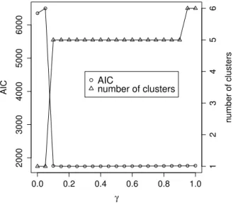
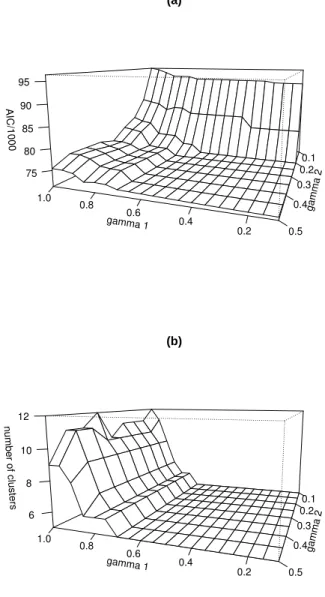
Figure 3.3 displays a sample from (a). We simulated 100 runs for each setting and compared clustering results from SC with those from theK-means clustering and MSC. Figure 3.4 shows the value of AIC and the number of clusters resulting from SC for the sample in Figure 3.3. The selected value of γ based on AIC was 0.15. To measure the performance of clustering, we used the biological homogeneity index (BHI) (Wu, 2011), which measures the homogeneity between the cluster _{C = {C}₁, . . . , CK} and the true category