Volume 31, Issue 3
Fiscal Policy under the Debt Feedback Rule: The Case of Japan
Jun-hyung Ko
Graduate School of Economics, Hitotsubashi University
Hiroshi Morita
Graduate School of Economics, Hitotsubashi University
Abstract
The Japanese government has amassed a huge amount of gross public debts over the past several decades. However, previous empirical works dealing with vector auto-regression (VAR) have not considered the effect of debt on fiscal policy and the macro economy. In this paper, we incorporate debt dynamics in a VAR model in the spirit of Favero and Giavazzi (2007, 2011). The inclusion of the debt feedback rule in VAR can help overcome the misspecification problem and provide direction toward a more relevant debt path and fiscal stance. The main findings of our study are as follows. First, in the pre-bubble period, the fiscal authority in Japan increased the primary surplus when the public debt level was high. However, this Ricardian behavior was not seen in the post-bubble period. Second, the impulse response functions to the expansionary government spending shock reveal that the stance of fiscal policy was more active in the pre-bubble. Third, while the forecast of debt dynamics in the pre-bubble period was stable, it became explosive in the post-bubble period.
We thank the associate editor of the journal, John P. Conley and an anonymous referee for their valuable comments and suggestions. Citation: Jun-hyung Ko and Hiroshi Morita, (2011) ''Fiscal Policy under the Debt Feedback Rule: The Case of Japan'', Economics Bulletin, Vol. 31 no.3 pp. 2373-2387.
Submitted: Apr 26 2011. Published: August 23, 2011.
1 Introduction
From the mid-1970s, govenment debt has been steadily increasing in Japan, thereby depressing the Japanese economy.1 In the early 1970s, Japan’s government debt for Japan was maintained at less than twenty percent of the annual GDP. However, since then, the debt stocks have surged to more than 200 percent in 2009. The rising debts may limit the effect of the government’s expansionary policy to stimulate the stumbling economy.
A number of empirical works have investigated the effect of fiscal policy shocks in the Japanese economy. Many of these studies adopt the VAR methodology to identify a pure fiscal policy shock. For example, Kuttner and Posen (2002), Bayomi (2001), and Ihori and Nakamoto (2005) analyze the effect of the expansionary fiscal policy on macro variables such as GDP and aggregate consumption. Most of these previous works use Cholesky decomposition to identify fiscal policy shocks. On the other hand, Watanabe, Yabu, and Ito (2011) and Kato (2003) adopt a Blanchard-Perotti type identification scheme: they rely on institutional information about tax and transfer systems and the timing of tax collections to identify the automatic response of taxes and government spending to economic activity. Recently, Miyazaki (2010) has followed the narrative approach introduced by Ramey and Shapiro (1998) to examine the fiscal policy effect during the 1990s. The general inference of these existing works is that an increase in government expenditure or a cut in government revenues had positive effects on output in the pre-bubble period, but the government’s expansionary effect was limited in the post-bubble period.
Through this study, our aim is to analyze the effect of fiscal policy in Japan while consider- ing debt feedback. The stance of fiscal policy is important because it reflects the future actions of the government, and the economy is also influenced by how the market expects the fiscal ac- tions. However, in the previous works with VAR models, the dynamics of public debt were not explicitly considered in the estimation.2 As discussed in Favero and Giavazzi (2007, 2011), this may result in a misspecification problem and hence, the forecast of the debt path may become irrelevant. In this paper, we employ the VAR methodology with an explicit inclusion of debt feedbacks following Favero and Giavazzi (2007, 2011). When estimating the VAR model, we explicitly incorporate the debt-to-GDP ratio as an explanatory variable. We also consider the fact that public debt evolves through the government’s inter-temporal budget constraint. Insti- tutional information was used to identify pure fiscal shocks. Following Watanabe et al. (2011), we split the sample period into pre- and post- bubble periods to discuss the changing pattern of fiscal effects.
Our main findings are as follows. First, in the first sample period, from 1970Q1 to 1986Q4, the fiscal authority tried to maintain a positive primary surplus when public debt was at a high level. However, this phenomenon was not seen in the post-bubble period, from 1987Q1 to 2004Q4. Although Japan is yet to pay back huge debts, the government has adopted the stance of increasing expenditures and decrease tax revenues. Second, the impulse response functions to the expansionary government spending shock reveal that the fiscal policy stance in the pre-bubble period was more active in reducing public debts. The government also in- creased the tax revenues in response to the increase in spending. Despite this negative wealth
1In this paper, government debt refers to the debt of the central and local governments. For the definition of debt, see the data section.
2The only exception is Ito, Watanabe, and Yabu (2011). Using the Markov-switching model, they examine how the fiscal authority reacts to the past debt level. However, they do not examine the effect of government policy on the economy.
effect on households, Japan has witnessed a significant expansion of its GDP. The correspond- ing debts response shows a decreasing pattern under the expansionary government spending shocks. However, in the second sub-sample period, the government did not increase taxes. Moreover, the expansionary effect on GDP was reduced. This is strongly related to debt dy- namics. Different from the first sample period, the response of debt becomes positive in the short run. This may induce a rather contractionary effect in the economy. However, these effects are not observed under the no feedback rule specification. In both periods, the gov- ernment does not increase taxes sufficiently. Third, under the debt feedback rule, the forecast of debt dynamics in the pre-bubble period was stable, reflecting the government’s Ricardian behavior. However, in the post-bubble period, the debt path becomes explosive owing to the government’s failure to stabilize debt. However, the simulated path under the no feedback rule exhibits a very different sequence: the path is explosive in the pre-bubble period and stable in the post-bubble period. Thus, we conclude that the explicit inclusion of the feedback rule is very important to estimate and analyze the effect of fiscal policy.
The rest of the paper is organized as follows. In Section 2, we review the Japanese economy and the Japanese government’s behavior from 1970 to 2004. In Section 3, we describe the VAR model with debt feedback and our identification scheme. In Section 4, we present our estimation and benchmark results. In Section 5, we conclude our paper.
2 Overview of the Japanese Government’s Expenditure and
Debt
2.1 The intertemporal government budget constraint
The flow government budget constraint on date t can be written as follows:
Dt= (1 + rt)Dt−1− St, (1)
where Dt denotes the nominal public debt at the end of date t, rt is the one-period nominal interest rate to be paid for the existing debt at the beginning of t, and St (≡ Tt− Gt) denotes the nominal primary surplus where Gt and Tt are the nominal government expenditures and revenues, respectively.3 When this equation is divided by the nominal GDP, the inter-temporal government budget constraint becomes
dt= q−1t dt−1− st, (2)
where dt is the debt-to-GDP ratio, qt (≡ 1+n1+rt
t) is a discount factor, nt is the nominal growth rate of GDP, and stis the primary surplus divided by GDP. The current debt-to-GDP ratio now depends on two terms: the past debt-to-GDP ratio divided by the discount factor and primary surplus-to-GDP ratio. Thus, the debt-to-GDP ratio is stabilized only when the discount factor or the primary surplus is sufficiently high.
2.2 Economic Performance and Fiscal Policy
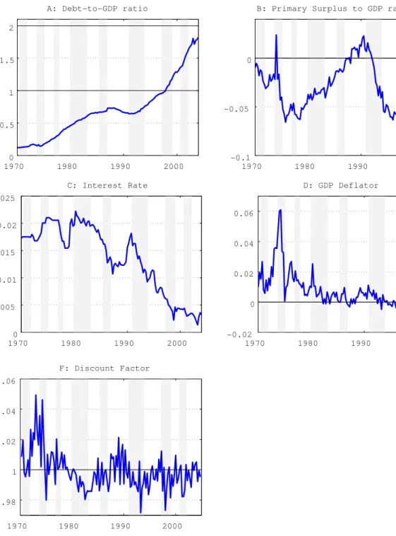
In this subsection, we briefly review the fiscal policy from the 1970s through the 2000s. Figure 1 displays the government’s and other related variables during this period.
3We assume that the seigniorage revenue is zero because the actual revenue was small.
Figure 1: Government’s Behavior and Economic Performance
1970 1980 1990 2000
0 0.5 1 1.5 2
A: Debt-to-GDP ratio
1970 1980 1990 2000
-0.1 -0.05 0
B: Primary Surplus to GDP ratio
1970 1980 1990 2000
0 0.005
0.01 0.015
0.02 0.025
C: Interest Rate
1970 1980 1990 2000
-0.02 0 0.02 0.04 0.06
D: GDP Deflator
1970 1980 1990 2000
0.98 1 1.02 1.04 1.06
F: Discount Factor
Note: The shaded areas indicate periods of economic recession.
Panel A in Figure 1 represents the debt-to-GDP ratio from 1970Q1 to 2004Q4. Since the mid-1970s, the debt-to-GDP ratio for Japan has seen a consistently increasing trend. The debt- to-GDP ratio was maintained at 10 to 20 percent of the annual GDP in the early 1970s. How- ever, since then, the debt-to-GDP ratio has increased steadily except at the peak of the bubble period in the late 1980s. In particular, after the ushering the 1990s, the so-called “lost decade,” Japan’s GDP performance was poor despite the huge volume of government spendings. Public debts finally exceeded the annual GDP in the late 1990s. In the new millennium, after Japan
had recovered to a certain degree, public debts had increased to almost twice as much as the GDP in 2004.
Panel B shows the primary surplus-to-GDP ratio. Throughout the sample period, the surplus- to-GDP ratio was generally negative owing to the fact that the volume of government expendi- tures exceeded government revenues, thereby leading to an increase in the debt-to-GDP ratio. However, its trend between the pre- and post- bubble periods are different. Starting from the late-1970s, the surplus-to-GDP ratio has shown an increasing pattern until the bubble burst in 1990, but it has shown a decreasing pattern thereafter. This means that authority’s management became more stringent entering 1990s. In the pre-bubble period, the government revenue was strictly increasing despite enlarged government spendings. In the post-bubble period, the size of government expenditures relative to GDP showed a strictly increasing pattern, while the tax revenues started to show a decreasing pattern in the post-bubble period.
Panels C and D each display the series of the interest rate on public debt payments and the inflation rate of the GDP deflator, respectively. Although public debt was skyrocketing, the interest rate shows an opposite shape. One of the main reasons for this was the stance of the Bank of Japan. In the mid-1980s, the uncollateralized overnight call rate was lowered to boost the economy and then increased in the late-1980s. Since 1991, to stimulate the economy, the Japanese government began lowering the call rate, which declined to 6.25 percent in December 1991, 3.82 in December 1992, 0.4 percent in December 1995, and 0.01 percent in 1999. Other interest rates, including the long-term Japanese government bond (JGB) yield also followed the sequence of the call rate.
Panel E plots the discount factor. Equation (2) shows that when the discount factor is low, the debt burden increases. Except for in the early 1970s and late 1980s, the discount factor has been less than one. The decreasing pattern of the discount factor in the 1970s and 1980s and its consistently low level since 1990 may account for some fraction of the increasing pattern of the debts in both periods.
3 Framework of Analysis
3.1 Traditional VAR with Fiscal Policy
Before the illustration of the VAR model with a feedback rule, we begin with a brief discussion on a standard VAR model:
Yt= β0,t+
p
∑
i=1
βiYt−i+ ut, (3)
Aut= Bεt, (4)
where Yt′ = [gt, τt, yt, πt, rt] is a (5×1) vector of the macro variables in the order of government expenditure, tax revenue, output, inflation, and interest rates.4 β0,t are deterministic terms including a vector of intercepts, time trends, and an oil-shock dummy, and βi (i = 1, · · · , p) are the matrices of coefficients. ut are the error terms of the reduced form, and εt are the
4Watanabe et al. (2011) use VAR models with three variables, government expenditure, tax revenue, and output and provide evidence that the government expenditure shock raised the GDP in the pre-bubble period.
structural shocks of interest.
1 0 agy agπ agr
0 1 aτ y aτ π aτ r
a31 a32 1 0 0 a41 a42 a43 1 0 a51 a52 a53 a54 1
ugt uτt uyt uπt urt
=
b11 0 0 0 0
b21 b22 0 0 0 0 0 b33 0 0 0 0 0 b44 0
0 0 0 0 b55
εgt ετt εyt επt εrt
, (5)
where we do not interpret the third to the fifth shocks. Using the external information, we identify agy, agπ, agr, aτ y, aτ π, and aτ r. Two output elasticities, agy and aτ y, are taken from Watanabe et al. (2011). Following Watanabe et al. (2011), we set agy = 0, because the automatic response of govenment expenditure to output fluctuations within a quarter is limited. Furthermore, Morita (2011) discusses that implementation lags exist in Japan. aτ y are set at 0.189 and 0.141 in the pre- and post-bubble periods respectively.5 The price elasticity of government spending depends on the decision of contracts: if the spending is fixed in nominal terms within a quarter, the elasticity is −1 and if it is based on real-good terms, the elasticity becomes zero. Favero and Giavazzi (2007) and Perotti (2005, 2007) assume that agπ = −0.5 in
the U.S. case, which lies among those values. Following Kato (2003), however, we assume that agπ = −1 because government spendings in Japan are generally fixed in nominal terms.6 For agrand aτ r, we follow the assumptions in Favero and Giavazzi (2007) and Perotti (2005, 2007). We assume that agr = aτ r = 0, because property income is excluded in both expenditure and revenue. The individual interest income may be related to the tax income. However, it may take more than one quarter to increase the tax revenue. We take the value of aτ π from Kato (2003).
The left 15 parameters are just identified because the estimated variance-covariance matrix of the five-equation VAR innovations contains 15 different elements. Finally, we assume that the second structural shock does not have an impact effect on government spending: b12= 0.
3.2 Impulse Responses
The vector-moving-average representation of the VAR model can be easily derived. Equation (3) can be written in a vector moving average form as
Yt= C(L)−1u˜t, (6)
where C(L) ≡ (I − β1L − · · · − βpLp) and ˜ut= β0,t+ ut. Therefore in a more compact form, it becomes
Yt = φt+ ζεt, (7)
where φt ≡ C(L)β0,t and ζ ≡ AC(L)−1B. Given the estimates of the coefficients and volatilities, we can calculate the measures of impulse responses (hereafter IR) of selected macro variables to structural shocks. This is done in the following steps. First, we generate a baseline simulation
5These values are relatively lower than those in the U.S. and other major OECD countries. Watanabe et al. (2011) document three related facts. First, the annual-based elasticity offered by the Ministry of Finance is 1.1, and there is a big discrepancy from the quarter-based elasticity. Second, the relative weights of income tax and corporate tax became bigger, while those of indirect tax were lowered. Third, consumption tax was introduced in 1989: the elasticity of consumption is almost zero.
6We also re-estimate the VAR model with the value agπ = −0.5 and we have a similar result.
for all variables by solving (3) dynamically forward. Second, we generate an alternative sim- ulation by setting to one percent deviation of the structural shock, and dynamically solve the model forward up to the same horizon used in the baseline simulation. Third, we compute IRs to the structural shocks as the difference between the simulated values in the two steps above. Fourth, we compute confidence intervals by bootstrapping, for example.
3.3 VAR with debt feedback
Now, the VAR specification includes the debt-to-GDP ratio (d) and the government intertem- poral budget constraint:
Yt= β0,t +
p
∑
i=1
βiYt−i+ γdt−1+ ut, (8)
where the debt-to-GDP ratio evolves in the following identity of the government intertemporal budget constraint:
dt = (1 + rt)
(1 + πt)(1 + ∆yt)dt−1+
exp(gt) − exp(τt)
exp(yt) , (9)
Aut = Bεt.
Note that the identification of structural shocks is not different from the standard VAR. No parameter is to be estimated in the government budget constraint. However, we include the feedback from public debt following Favero and Giavazzi (2007). This specification is impor- tant in analyzing the effect of fiscal policy shocks. Woodford (1998), Bohn (1998), and recently Ito et al. (2011) have analyzed whether the fiscal policy is adopting a Ricardian behavior. If the government is reacting to past debts and attempting to stabilize the debt-to-GDP ratio, the feedback rule of government spending and revenue from the past level of the debt-to-GDP ratio is expected. Furthermore, government spendings and revenues, interest rates, real GDP growth, inflation are linked by the government’s intertemporal budget constraint. Debt dynam- ics may influence interest rates and inflation. The relationship between debts and monetary variables may reflect the policy-stance relationship between the monetary and fiscal authori- ties. The debts accumulated in the past may influence output and other macro variables such as consumption because debts have to be stabilized in the end. Therefore, it is important to incorporate these relationships through the intertemporal government budget constraint.
4 Estimation and Benchmark Results
4.1 Data
We employ the quarterly data of five selected macro variables, and the sample period is 1970Q1 to 2004Q4. The series of government expenditure, tax revenue, and real GDP are taken from Watanabe et al. (2011). These variables are seasonally adjusted and in per capita. For the inflation data, we take the log differences of the seasonally adjusted GDP deflator downloaded from the SNA database. We use interest rates and public debt data from Zaisei Kinyuu Tokei Geppo (Ministry of Finance Statistics Monthly). We define government debts as the sum of government bonds, financing bills, borrowings, and temporary borrowings. However, the data
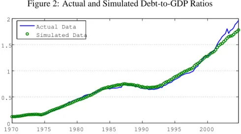
Figure 2: Actual and Simulated Debt-to-GDP Ratios
1970 1975 1980 1985 1990 1995 2000
0 0.5
1 1.5
2
Actual Data Simulated Data
Notes: The blue line represents the actual data, and the green circled line represents the simulated data.
from Zaisei Kinyuu Tokei Geppo only covers the debts issued by the central government, and hence, we collect data related to the local governments from the homepage of the Ministry of Finance in Japan.7 For interest rates, we use the JGB yield.
Figure 2 compares the actual and simulated data. The simulated data of debts was con- structed from the government budget constraint in equation (2), taking the actual value of debt in 1970Q1 as an initial value, dt−1. The simulated data closely traces the actual data. However, some deviation is observed in the later period. This is probably due to the burden of social transfers, such as pension benefits, that is not considered in our model.
We split the total samples into two sub-sample periods: from 1970Q1 to 1986Q4 and from 1987Q1 to 2004Q4. The occurrence of the structural shift around 1987, the onset of the bub- ble period, is often discussed in the existing works such as Jinushi et al (2000). This can be criticised because of the degrees of freedom originating from the relatively short sub-sample periods.8 However, we estimate two sub-sample periods because one of the main purposes in our study is to compare our debt feedback rule VAR with the related preceeding literature. Four lags are suggested by the Akaike information criterion in both of the sub-sample periods. The VAR is estimated by using equation-by-equation least squares.
4.2 Activity of Fiscal Authority Stance
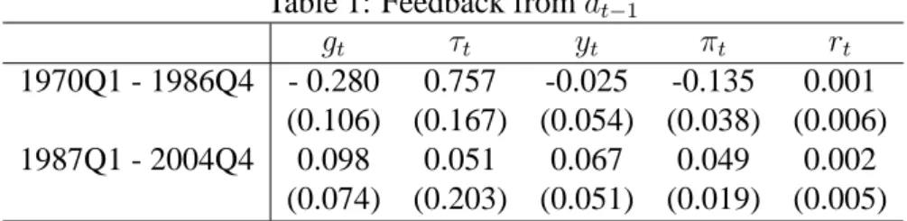
We start by interpreting the estimated coefficients of the debt-to-GDP ratio in the VAR model. Table 1 reports the results of the two sub-samples.
The estimated coefficients of the debt to government expenditure and tax revenue reflect how actively the government reacted to the past debt level in each sample period. In the pre- bubble period, we observe a sigficantly positive response of the primary surplus to the past debt- to-GDP ratio. In response to the previous debt level, the government increased tax revenues and decreased its spendings to stabilize the economy. In particular, the stabilizing effect of
7Since only annual data related to the local governments is available, we assume that the share of the local governments’ debts is constant.
8We thank an anonymous referee for suggesting that we seriously consider this problem. However, the local government data is available since 1970Q1. We leave this issue on the future research.
Table 1: Feedback from dt−1
gt τt yt πt rt
1970Q1 - 1986Q4 - 0.280 0.757 -0.025 -0.135 0.001 (0.106) (0.167) (0.054) (0.038) (0.006) 1987Q1 - 2004Q4 0.098 0.051 0.067 0.049 0.002
(0.074) (0.203) (0.051) (0.019) (0.005)
Note: The standard errors are in parenthesis.
primary surplus on debts works mainly through the government’s response of increasing tax revenue. This active stance of the fiscal authority leads to a negative but insignificant sign of output. This is because the increase in tax revenues is linked to the negative wealth effects on households.
In the second sub-sample period, there is no evidence supporting the argument that the gov- ernment adopts a Ricardian behavior. The government’s spending had considerably increased in response to the past debt-to-GDP ratio. The tax revenue had increased but not significantly. The expansion of government spendings is positively related to output. However, the volume of the output is smaller than the primary deficit volume. In all cases, the response of the interest rates is positive but insignificant.
4.3 IRs in Each Subsample
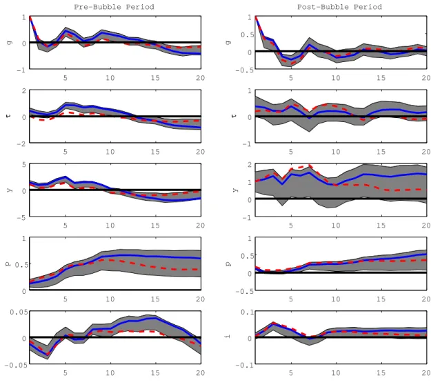
In this subsection, we examine the effectiveness of the expansionary government spending shock and the responsiveness of the fiscal policy to the need in financing government expen- diture. Figure 3 shows the evolution of the responses to government spending shocks in two sub-sample periods: the pre-bubble period in the left column and post-bubble period in the right column. For each period, we collect the IRs for the 20 periods of the horizons. The solid blue and dashed grey lines indicate the estimated IRs and one standard-error bootstrapped con- fidence intervals, respectively, under the debt feedback rule. The red dash-dotted lines are the estimated IRs of each variable under the no feedback rule.
We start by looking at the IRs under the feedback rule. As can be seen in the third row, the expansionary government shocks are found to have positive effects on the GDP in the pre- bubble period. However, these effects become insignificant in the post-bubble period, similar to the findings in the preceding literature. More importantly, the expansion of government spending leads to the increase of tax revenues in the pre-bubble period. This means that the government increased taxes rather than issuing new debts during this period. However, this Ricardian behavior of the government was not observed in the second sample period. In the latter period, the government relied more on the debts to finance the expenditure in the latter period.
Figure 3: IRs with Feedback and No Feedback
5 10 15 20
-1 0 1
g
Pre-Bubble Period
5 10 15 20
-0.5 0 0.5
1
g
Post-Bubble Period
5 10 15 20
-2 0 2
τ
5 10 15 20
-1 0 1
τ
5 10 15 20
-5 0 5
y
5 10 15 20
-1 0 1 2
y
5 10 15 20
0 0.5
1
p
5 10 15 20
-0.5 0 0.5
1
p
5 10 15 20
-0.05 0 0.05
i
5 10 15 20
-0.1 0 0.1
i
Note: The solid blue lines and shade areas indicate the estimated IRs and one standard-error bootstrapped confidence intervals, respectively, under the debt feedback rule. The red dash-dotted lines represent the estimated
IRs of each variable under the no feedback rule.
The IRs under the no feedback rule are generally the same as those in the debt feedback case in both periods. In the case when we do not include the debt feedback, the effect of expansionary government expending shocks on GDP is also positive in the short run. We observe persistently positive effects of government expenditure shocks on inflation in both periods. IRs of interest rates, which are the cost of servicing the debt, are positive.
However, there is one distinctive difference between two periods. Even in the pre-bubble period, taxes were not increased greatly and they were even lowered in the first four periods. The government does not increase the tax revenue in response to its expenditures. In other words, debts are issued to finance government expenditures. In the no-feedback rule case, the positive effect on GDP is lower compared to the feedback case.
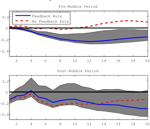
To discuss this difference between the two specifications in greater detail, Figure 4 displays the IRs of debts. Under the feedback rule, expansionary government expenditure shocks boost the economy so that the government could collect considerable tax revenues in the pre-bubble
Figure 4: IRs of Public Debt
2 4 6 8 10 12 14 16 18 20
-0.4 -0.2 0 0.2
Pre-Bubble Period
Feedback Rule No Feedback Rule
2 4 6 8 10 12 14 16 18 20
-0.4 -0.2 0 0.2
Post-Bubble Period
Note: The solid blue lines and shade areas indicate the estimated IRs and one standard-error bootstrapped confidence intervals, respectively, under the debt feedback rule. The red dash-dotted lines represent the estimated
IRs of each variable under the no feedback rule.
period. Therefore, the debts had reduced substantially. However, tax revenue responses are negligible in the second sub-sample period. Thus, the debt responds positively. IRs under the no feedback rule cannot capture this effect.
4.4 Debt Forecast
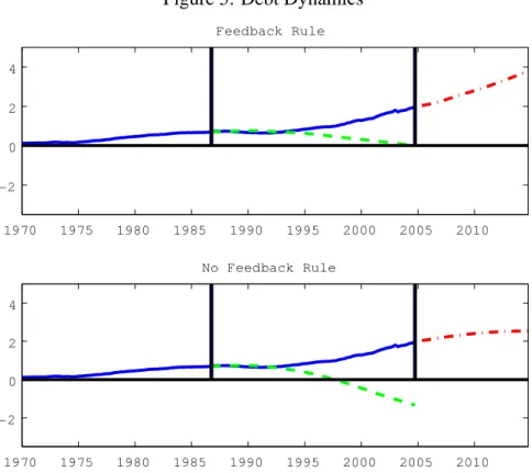
Figure 5 exhibits the debt forecast obtained from the intertemporal government budget con- straint in the two sub-sample periods.
When we consider the feedback rule of debts, the expected path of debts in the out-of- sample period is relatively stationary in the pre-bubble period. The Ricardian behavior of the government stabilized the economy so that there was no extreme path of debt levels. This result is consistent with that in Table 1. In the case of no feedback of debts, the forecast of the debt path in the pre-bubble period shows a sharply negative path. This means that the government is expected to become not a borrower but a saver with extremely positive wealth gains, which is unrealistic.
Figure 5: Debt Dynamics
1970 1975 1980 1985 1990 1995 2000 2005 2010 -2
0 2 4
Feedback Rule
1970 1975 1980 1985 1990 1995 2000 2005 2010 -2
0 2 4
No Feedback Rule
Note: The blue lines represent the actual debt-to-GDP ratio path. The green dashed lines represent the forecast of the debt-to-GDP ratio in the pre-bubble period. The red dash-dotted lines represent the forecast in the
post-bubble period.
A contradictory phenomenon is observed in the post-bubble period. The out-of-sample simulation under the no feedback rule exhibits a considerably stabilized path of the debt-to- GDP ratio. However, the debt path under the feedback rule diverges at a high speed. As discussed in Table 1, in the second sub-sample period, the government had adopted a non- Ricardian behavior so that the debt yielded an unstable path. However, the debt path under the no feedback rule is relatively stable. Therefore, we can conclude that omitting a feedback rule can result in very different paths for the debt-to-GDP ratio.
5 Robustness
For the robustness check, we carry out two alternative estimations. In the benchmark case, we estimate the VAR model with a deterministic time trend. First, in our first robustness check, we re-estimate the model without a time trend. Second, as an explanatory variable, we use the difference of the debt-to-GDP ratio rather than the past level. Overall, the results are the same as those in the benchmark case. Therefore, we exhibit the coefficients of debts. Tables 2 and 3 show the results of the first and second robustness checks respectively.
In all cases, we find significant evidence that the government adopts a Ricardian behavior in the pre-bubble period. However, there is no evidence to support this phenomenon in the post- bubble period. In most cases, the coefficients for the government variables are not statistically significant in the latter period.
Table 2: Feedback from dt−1with no time trend
gt τt yt πt rt
1970Q1 - 1986Q4 - 0.160 0.503 0.010 -0.134 -0.003 (0.119) (0.161) (0.047) (0.032) (0.005) 1987Q1 - 2004Q4 -0.015 -0.048 0.004 -0.003 0.000
(0.011) (0.027) (0.007) (0.003) (0.001)
Note: The standard errors are in parentheses.
Table 3: Feedback from∆dt−1
gt τt yt πt rt
1970Q1 - 1986Q4 0.419 0.856 -0.035 0.005 -0.030 (0.364) (0.656) (0.175) (0.142) (0.019) 1987Q1 - 2004Q4 -0.012 0.075 -0.056 -0.004 0.004
(0.079) (0.214) (0.054) (0.021) (0.006)
Note: The standard errors are in parentheses.
6 Concluding Remarks
Japan’s public debt level surged to more than 200 percent of the GDP in 2009, limiting the government’s ability to spend more to revive growth. The rising debt-to-GDP ratio is a treat for the Japanese economy. However, in the existing empirical papers with VAR models the debt effect was not fully considered while estimating fiscal shocks. In this paper, we analyze the effectiveness of the Japanese fiscal policy under the existence of debt feedback in the pre- and post-bubble periods. In contrast to the previous VAR literature with no feedback of debts, our model allows us to detect the changes in the fiscal policy mechanisms between two sample periods.
Three main conclusions can be drawn from our analysis. First, the explicit inclusion of debt feedback allows us to study how actively the fiscal authority responded to the past debt level. In the pre-bubble period, the government actively tried to stabilize the debt level by increasing tax revenues and decreasing government spending. On the other hand, the government increased spending despite the high level of debts in the post-bubble period. Second, IRs on government spending shocks support the first finding: the Ricardian behavior of the government in the pre-bubble period. In response to the exogenous government spending shocks, tax revenues were raised significantly. Although the interest payments increased, output and inflation also increased. This reduced the burden of debt payments. The positive primary surplus also lowers the volume of debts. However, we cannot find this evidence under the no feedback rule. Third, from the out-of-sample exercise, we find that the dynamics of the debt-to-GDP ratio under the feedback rule were rather stable compared to the no feedback case in the pre-bubble period. However, the dynamics of debt-to-GDP ratios are overestimated under the no feedback rule. In the post-bubble period, the VAR model with debt feedback reveals that the government’s stance on the debt level shows a very unstable path. It is underestimated under the no feedback rule. Therefore, we conclude that the estimation of the VAR model without the inclusion of debt feedback may result in the adoption of an unrealistic path of debt dynamics and a wrong policy stance.
Reference
Bayoumi, T., (2001): “The Morning After: Explaining the Slowdown in Japanese Growth in the 1990s,” Journal of International Economics, 53 (2), 241-259.
Blanchard, O. and R. Perotti, (2002): “An Empirical Characterization of the Dynamic Effects of Changes in Government Spending and Taxes on Output,” Quarterly Journal of Economics, 117 (4), 1329-1368.
Bohn, H., (1998): “The Behaviour of U.S. Public Debt and Deficits,” Quarterly Journal of Economics, 113, 949-963.
Chung, H. and D. Leeper, (2010): “What has Financed Government Debt?” NBER Working Paper, 13425, National Bureau of Economic Research, Inc.
Favero, C. A. and F. Giavazzi, (2011): “Reconciling VAR based and Narrative Measures of the Tax Multiplier,” American Economic Journal. Economic Policy, forthcoming.
Favero, C. A. and F. Giavazzi, (2007): “Debt and the Effects of Fiscal Policy,” NBER Working Paper, 12822, National Bureau of Economic Research, Inc.
Ihori, T. and A. Nakazato, (2005): “Japan’s Fiscal Policy and Fiscal Reconstruction,” Interna- tional Economics and Economic Policy, 2 (2-3), 153-172.
Ito, A., Watanabe, T., T. Yabu, (2011): “Fiscal Policy Switching in Japan, the U.S., and the U.K.,” Understanding Inflation Dynamics of the Japanese Economy Working Paper Series No. 70.
Kato, R., (2003): “Zaisei Jousuuno Nichibei Hikaku: Kouzou VAR to Seidoteki Youinwo Heiy- ousita Approach”, IMES working paper series, 03-J-4. (In Japanese)
Kuttner, K. N. and A. S. Posen, (2002), “Fiscal Policy Effectiveness in Japan,” Journal of the Japanese and International Economies, 16 (4), 536-558.
Jinushi, T., Y. Kuroki, and R. Miyao, (2000): “Monetary Policy in Japan Since the Late 1980s: Delayed Policy Actions and Some Explanations,” Japan’s Financial Crisis and its Parallels to US Experience.
Miyazaki, T., (2010): “The Effects of Fiscal Policy in the 1990s of Japan: VAR Analysis with Event Studies,” Japan and World Economy, 22 (2), 80-87.
Morita, H., (2011): “The Effects of Fiscal Policy in Japan: Expectation-Augmented VAR Anal- ysis,” mimeo (in Japanese).
Mountford, A. and H. Uhlig, (2002): “What Are the Effects of Fiscal Policy Shocks?” CEPR Discussion Paper 3338.
Perotti, R., (1999): “Fiscal Policy in Good Times and Bad,” Quarterly Journal of Economics, 114 (4), 1399-1439.
Perotti, R., (2005): “Estimating the Effects of Fiscal Policy in OECD Countries,” CEPR Dis- cussion Paper, 4832.
Perotti, R., (2007): “In Search of the Transmission Mechanism of Fiscal Policy,” NBER Macroe- conomics Annual, 22, 169-226.
Ramey, V. A. and M. D. Shapiro, (1998): “Costly Capital Reallocation and the effects of gov- ernment spending,” NBER Working Paper, N0. 6283, National Bureau of Economic Research, Inc.
Woodford, M, (1998): “Public Debt and the Price Level,” Princeton University.
Watanabe, T., T. Yabu, and A. Ito, (2011): “Estimation of the Fiscal Multiplier based on In- stitutional Information,” Ihori, T. Fiscal Policy and Social Insurance. Economic and Social research institute, Cabinet office, Government of Japan (in Japanese).