TA8 最近の更新履歴 Econometrics Ⅰ 2016 TA session

TA session# 8

Jun Sakamoto

June 14,2016

Contents

1

Introduction of GLS 1

2

OLSE and GLSE 3

1 Introduction of GLS

The following items were suppoused about error term in OLS.

A.E[ui] = 0 B.E[u²_i] = σ²< ∞ C.E[uiuj] = 0, ∀i 6= j

But we often confront the situation that above assumption dose not hold.

Example1:Heteroscedasticity

If error term has different variance, then variance-covariance matrix was represent as below.

σ²Ω =













σ1² 0 · · · 0 0 σ²2 . .. ... ... . .. ... 0 0 · · · 0 σ²_n











 Example2:First-Order Autococorrelation

If error term has firs-order autocorrelation(i.e.ut= ρu_t−1+ ǫt), then then variance-covariance matrix was rep- resent as below.

σ²Ω = _1−ρ^σ2ǫ2















1 ρ ρ² · · · ρⁿ⁻¹ ρ 1 ρ · · · ρⁿ⁻² ρⁿ⁻² ρ 1 · · · ρⁿ⁻³

... ^... ^... ^{. .. ..}. ρⁿ⁻¹ ρⁿ⁻² ρⁿ⁻³ · · · 1















OLS is not BLUE above mentioned but GLS is BLUE.

Ω is a matrix of symmetric and real number. So we can diagonalize Ω,

Ω = A^′ΛA = CC^′(C = A^′Λ^1/2) Λ is a diagonal matrix and the diagonal elements are the eigenvalue. Ais a consisting of eigen vectors.

(If you don’t understand above, please check 2nd lecture note.) Regression model is,

y= Xβ + u. Multiply C⁻¹ on both sides of regression model.

C⁻¹y= C⁻¹Xβ+ C⁻¹u ←→ y^∗= X^∗β+ u^∗ Therefore we can get a bellow estimater.

βˆGLS= (X^′Ω⁻¹X)⁻¹X^′Ω⁻¹y Error term of new regression model is homoscedastic.

E[uu^′] = C⁻¹E[uu^′]C^′−1

= C⁻¹σΩC^′−1 σ²C⁻¹ΩC^′−1

= σ²In

Property8.1

(1)E[ ˆβGLS] = β (2)V [ ˆβGLS] = σ²(X^′Ω⁻¹X)⁻¹ Proof(1)

βˆ_GLS= (X^′Ω⁻¹X)⁻¹X^′Ω⁻¹y

= (X^′Ω⁻¹X)⁻¹X^′Ω⁻¹(Xβ + u)

= β + (X^′ΩX)⁻¹X^′Ω⁻¹u Thus, take expectation

E[ ˆβGLS] = E[β + (X^′Ω⁻¹X)⁻¹X^′Ω⁻¹u] = β

Q.E.D

2

Proof(2)

V[ ˆβGLS] = E[((X^′Ω⁻¹X)⁻¹X^′Ω⁻¹u)((X^′Ω⁻¹X)⁻¹X^′Ω⁻¹u)^′]

= E[(X^′Ω⁻¹X)⁻¹X^′Ω⁻¹uu^′Ω⁻¹X(X^′Ω⁻¹X)⁻¹]

= (X^′Ω⁻¹X)⁻¹X^′Ω⁻¹E[uu^′]Ω⁻¹X(X^′Ω⁻¹X)⁻¹

= (X^′Ω⁻¹X)⁻¹X^′Ω⁻¹σ²ΩΩ⁻¹X(X^′Ω⁻¹X)⁻¹

= σ²(X^′Ω⁻¹X)⁻¹X^′Ω⁻¹X(X^′Ω⁻¹X)⁻¹

= σ²(X^′Ω⁻¹X)⁻¹

Q.E.D Aitken Theorem

GLSE is a best linear unbiased estimator.

V[ ˆβGLS] ≤ V [b] for any linear unbiased estimator b. Proof

We can show that GLSE is BLUE like proof of the case that OLSE is BLUE because assumption is generalized by diagonalization.

Q.E.D

2 OLSE and GLSE

Property8.2

(1)OLSE is a unbiased estimator under the situation of the error term assumption does not satisfy B and C. (2)V [ ˆβGLS] ≤ V [ ˆβOLS]

Proof(1)

[ ˆβOLS] = (X^′X)⁻¹X^′y

= β + (X^′X)⁻¹X^′u

Above equation is also maintained under the heteroscedasticity. So we can show unbiasedness from assumption of A.

Q.E.D Proof(2)

Prop8.2 (2) is trivial because GLSE is BLUE.

V[ ˆβOLS] = E[((X^′X)⁻¹X^′u)((X^′X)⁻¹X^′u)^′]

= E[(X^′X)⁻¹X^′uu^′X(X^′X)⁻¹]

= (X^′X)⁻¹X^′E[uu^′]X(X^′X)⁻¹

= (X^′X)⁻¹X^′σ²ΩX(X^′X)⁻¹

= σ²(X^′X)⁻¹X^′ΩX(X^′X)⁻¹ Thus,

V[ ˆβOLS] − V [ ˆβGLS] = σ²(X^′X)⁻¹X^′ΩX(X^′X)⁻¹− σ²(X^′Ω⁻¹X)⁻¹

= σ²((X^′X)⁻¹X^′−(X^′Ω⁻¹X)⁻¹X^′Ω)Ω((X^′X)⁻¹X^′−(X^′Ω⁻¹X)⁻¹X^′Ω)^′

= σ²AΩA^′. Ω is positive definite matrix, AΩA^′ >0. Thus V [ ˆβGLS] ≤ V [ ˆβOLS]

Check variance of OLSE and GLSE.

1.We generate samples X ∼ U [0, 5] and u(u does not satisfy B or C).(t=50) 2.y is made by X and u from step1.(We assume true beta is 2)

3.We estimate ˆβ.

4. ˆβ is obtained by repeating above steps n times.

Example(1)

u1^{= (u1, ..., u25), ui∼ N(0, 1)}

u_{2= (u26, ..., u50), uj∼ N(0, 25)}

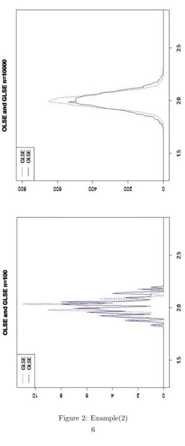
Example(2)

u_{1= (u1, ..., u25), ui∼ N(0, 1)} u_{2= (u26, ..., u50), uj∼ N(0, 4)}

Example(3)

ut= 0.8u_t−1+ ǫt, ǫt∼ N(0, σ²_t)

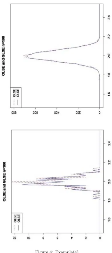
Example(4)

ut= 0.2u_t−1+ ǫt, ǫt∼ N(0, σ²_t)

4

Figure 2: Example(2) 6

Figure 4: Example(4)

8