A New Data Structure for SAT-Based Static Learning with Impact on Test Generation
1Emil Gizdarski*2 and Hideo Fujiwara**
* Department of Computer Systems, University of Rousse, Bulgaria
** Graduate School of Information Science, Nara Institute of Science and Technology, Japan
Abstract. In this paper we propose a new data structure for the complete implication graph that allows efficient deriving and performing static indirect ∧-implications. In this way, some hard-to-detect static indirect implications can be easily found during static learning. In addition, the static indirect ∧-implications are used to perform (without spare operations) some dynamic indirect implications during branch and bound search and dynamic learning.
1 This paper was supported by JSPS under grant P99747.
2 Currently visiting at Nara Institute of Science and Technology
1. Introduction
In recent years substantial progress has been achieved in CAD using the Boolean satisfiability (SAT) method. The main reason for this progress is development of efficient learning techniques. Learning play a key role in avoiding backtracking during branch and bound search by finding as many as possible necessary assignments at the current level. Many indirect implications can be easily derived during static learning, while high level recursive learning has to be applied to find them during branch and bound search. Previous works in test generation also showed that with efficient preprocessing, it is not necessary to perform dynamic learning for the vast majority of faults. Therefore, low complexity static learning is an important preprocessing phase for test generation.
2. Basic learning rules [1]
The contradiction and recursive learning are well-known learning rules called here rule 1 and rule 3.N where N determines the level of recursion. Using an unjustified line concept, some necessary assignments can be derived as an intersection of the conditions for satisfying a k-nary clause. This is called here an indirect ∧-implication or learning rule 2.
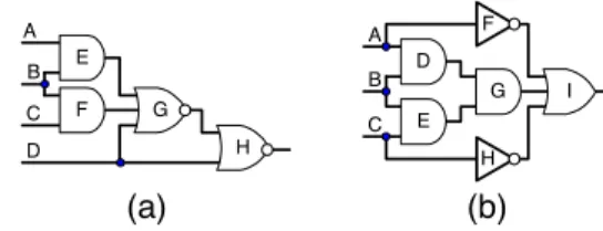
Figure 1(a) provides an example how the static learning procedure based on rule 2 finds indirect implication (H=1 → B=1). First, assignment H=1 binds variables D and G to 0 and k-nary clause (E ∨ F ∨ D ∨ G) is still unsatisfied. To satisfy this clause either variable E or F must be set to 1, but both these assignments imply that variable B should be set to 1. Therefore B=1 is a necessary assignment. Thus, indirect implication (H=1
→ B=1) is found. This implication cannot be found by rule 1. A super gates extraction can be used to find some indirect implications that cannot be found by rules 1 and 2. For the circuit in Figure 1(b), gates D, E and G form a super gate. If we replace these three gates by their super gate (3-input AND gate), then indirect implications (I=0 → B=0) and (B=1 → I=1) can be found by rule 1 (contradiction). In the original circuit, these indirect implications can be found by rule 3.1.
3. New data structure of implication graph
A new data structure of the complete implication graph represents each gate (k-nary clause) by 2k ∧-nodes, k direct ∧-
implications and one k-bit key dynamically calculated by the binding procedure, see Figure 2(a). For the basic gates, each bit of a k-bit key corresponds to one of the variables in a k-nary clause. The bit is set to one if this variable is specified and the clause is still unsatisfied. The k-bit key also has one extra bit, not presented in Figure 2(a), set to 1 when the clause is satisfied. This data structure can be easily manipulated and allows a unified representation of all k-nary clauses.
Example 1: Let us consider how indirect implication (H=1
→ B=1) in Figure 1(a) can be easily derived using the new structure of the complete implication graph. First, assignment B=0 binds variables E and F to 0 and k-nary clause (E ∨ F ∨ D
∨ G) is still unsatisfied. To take into account this new relation, the learning procedure adds static indirect ∧-implication B=1 to
∧-node <0011> of gate G, see Figure 2(b). Next, assignment H=1 binds variables D and G to 0 and the k-nary clause (E ∨ F
∨ D ∨ G) is still unsatisfied. To take into account this new relation, the learning procedure adds static indirect ∧- implication H=0 to ∧-node <1100> of gate G, see Figure 2(b). Clearly, the superposition of these two keys, <0011> and
<1100>, will result in <1111>, therefore these two assignments are inconsistent, i.e., if both assignments are preformed then all variables of this k-nary clause will be specified and the clause will be still unsatisfied. In this way, the static learning procedure easily finds indirect implication (H=1 → B=1).
Example 2: Figure 3 provides an example how the driving of static indirect ∧-implications and super gate extraction affect branch and bound search and dynamic learning. As a result of static learning based on rule 2, only one indirect ∧-implication is found for the iredundant circuit in Figure 3(a). After Figure 1: Network examples 1 and 2
Figure 2: The representation of static ∧-implications
Figure3: A network example 3 before and after super gate extraction
E C F B
D A
G H
(a) (b)
D
C E
B I
A
G F
H
I H G F
J
H G F
J C
D=0 B
E A
C D=0 B
E A
(a) (b)
(a)
F=1 1 1 1 1 1 1 1 0 1 1 0 1 1 1 0 0 1 0 1 1 0 1 1 1 0 0 1 1
CONFLICT
0 0 0 0 INITIALIZATION G=1 D=1
H=0
E=1 B=1
(b)
A=0 1 1 1 1 1 0 1 0 1 1 0 0 0 1 1 0 1 0 0 0 1 0 0 0
CONFLICT
INITIALIZATION B=0
C=1
A B C (A∨B∨C) A
B C
F D
(E∨F∨D∨G) G
E F D G E
IEEE European Test Workshop (ETW 2000), pp. 313-314, May 2000.
assignment D=0, this static indirect ∧-implication becomes a valid dynamic indirect implication (I=1 → B=1). Using this dynamic implication, implication (J=1→ B=1) can be found by dynamic learning based on rule 3.1 (first level recursive learning), otherwise dynamic learning based on rule 3.2 (second level recursive learning) must be applied. This implication can be found without dynamic learning if super gates are extracted before static learning. In this case, gates I and J form super gate J, see Figure 3(b), and dynamic indirect implication (J=1 → B=1) become valid after assignment D=0.
4. Experimental results
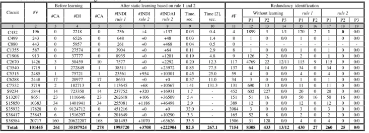
We implemented the new data structure in an implicit static learning procedure and ran experiments on a 450MHz Pentium- III PC. Table 1 shows the number of variables (V), constant assignments (CA), direct implications (DI), static indirect implications (INDI) and static indirect ∧-implications (INDAI) before and after static learning by rule 1 and rule 2. The contribution of learning rule 2 was 3708 static indirect implications and 222904 static indirect ∧-implications. We counted the implications as in [2]: (1) if a variable set itself and X other variables then X+1 implications were counted; and (2) the constant value assignments were not counted as implications after static learning. An indirect ∧-implication was countered if an assignment set at least two variables in a k-nary clause. Columns (10) and (11) provide CPU time of the implemented static learning procedure based on rule 2 with the equivalent static learning procedure of Simprid [2] (ran on HP 9000 J200). Our learning procedure was about 20 times faster than Simprid.
To evaluate the impact of the new data structure on test generation, we used the combinational ATPG system SPIRIT[3] for redundancy identification. SPIRIT is based on the Boolean satisfiability method and the Single Path Oriented Propagation (SPOP) method. Since SPIRIT processes a single output circuit, it is necessary to prove that a fault is redundant in respect to each primary output where the fault effect can be observed. Therefore, more than one test session for some faults had to be performed. As a criterion we chose three parameters: (P1) the maximum number of value assignments within one test session, (P2) the number of sensitized unjustifiable propagation paths and (P3) the number of aborted test sessions/faults. Columns (11-19) show the results in three cases: (case 1)
without static learning, (case 2) static learning based on rule 1 and (case 3) static learning based on rule 2. For learning rule 1 (learning rule 2), the maximum number of assignments was 430 (260) and the number of sensitized unjustifiable propagation paths was 27 (25). For these two parameters, the contribution of rule 2 was 40% and 7.4% respectively.
Let us assume that the preprocessing time is negligible in respect to the time spend for branch and bound search. Since we did not apply dynamic learning and search pruning techniques in this experiment then the number of assignments (the size of decision tree) can be associated with the complexity for redundancy identification. Therefore with the above- mentioned assumptions, the maximum number of assignments (P1) gives an idea about impact of the precision of static learning on the worst-case complexity for the redundancy identification. We observed two cases where a reduction of 170 and 2 times in parameter P1 was achieved after applying rule 2, for the circuit C432 and C1908. We also observed two cases where the number of the sensitized unjustifiable propagation paths were decreased after applying learning rule 2, for the circuit C432. In all cases, the effect was from the performing the static indirect ∧-implications (dynamic indirect implications) during SPOP. All these results demonstrate the efficiency of the new data structure of the complete implication graph for deriving and performing the indirect ∧-implications. We expect that the contribution of the new data structure will be more visible when super gate extraction is also implemented.
References:
[1] E.Gizdarski and H.Fujiwara, "A New Data Structure for Complete Implication Graph with Application for Static Learning," technical report NAIST-01, Jan.2000, pp.18. http://isw3.aist-nara.ac.jp/IS/TechReport2/report/2000001.ps
[2] J.Zhao, E.Rudnick and J.Patel, "Static Logic Implication with Application to Redundancy Identification," Proc. IEEE VLSI Test Symposium, 1997, pp. 288-293.
[3] E.Gizdarski and H.Fujiwara, "SPIRIT: Satisfiability Problem Implementation for Redundancy Identification and Test Generation," technical report NAIST-05, Apr.2000, pp.11. http://isw3.aist-nara.ac.jp/IS/TechReport2/report/2000005.ps
Table 1: Results static learning and redundancy identification
Before learning After static learning based on rule 1 and 2 Redundancy identification
Without learning rule 1 rule 2 Circuit #V
#CA #DI #CA #INDI
rule 1
#INDI rule 2
#INDAI rule 2
Time, sec.
Time [2],
sec. #F P1 P2 P3 P1 P2 P1 P2 P3
1 2 3 4 5 6 7 8 9 10 11 12 13 14 15 16 17 18 19
C432 196 0 2218 0 236 +4 +137 0.03 0.4 4 1899 3 1/1 170 2 1 0 0/0
C499 243 0 6526 0 648 +0 +48 0.03 1.4 8 1 0 0/0 1 0 1 0 0/0
C880 443 0 5957 0 261 +0 +468 0.04 0.5 0 - - - - - - - -
C1355 587 0 27574 0 3904 +0 +64 0.11 2.9 8 1 0 0/0 1 0 1 0 0/0
C1908 913 0 37777 0 8935 +0 +1201 0.19 4.8 9 126 2 0/0 2 0 1 0 0/0
C2670 1426 3 50459 10 7577 +0 +2292 0.20 12.3 117 4769 22 12/11 115 9 115 9 0/0
C3540 1719 1 272849 1 38511 +0 +23972 0.85 77.5 137 64 14 0/0 34 0 34 0 0/0
C5315 2485 1 75721 1 23561 +954 +10301 0.45 25.0 59 4 0 0/0 4 0 4 0 0/0
C6288 2448 17 20977 17 8633 +0 +0 0.37 11.0 34 3 0 0/0 1 0 1 0 0/0
C7552 3719 2 182713 4 113645 +68 +10567 1.41 131.3 131 690 13 0/0 11 0 11 0 0/0
S9234 5844 14 723350 14 237752 +320 +16931 1.7 - 452 602 227 0/0 20 0 20 0 0/0
S13207 8651 23 1116646 23 262618 +106 +36509 5.4 - 151 51 16 0/0 50 16 50 16 0/0
S15850 10383 34 1401941 34 255081 +1186 +46498 2.9 - 389 12 0 0/0 12 0 12 0 0/0
S35932 17828 0 9124712 0 451216 +0 +0 32.0 - 3984 3 0 0/0 3 0 3 0 0/0
S38417 23843 6 1516297 6 201649 +0 +10290 3.3 - 165 52 8 0/0 2 0 2 0 0/0
S38584 20717 160 20622207 168 381493 +1070 +63626 33.5 - 1506 31 128 0/0 4 0 4 0 0/0
Total: 101445 261 35187924 278 1995720 +3708 +222904 82.5 267.1 7154 8308 433 13/12 430 27 260 25 0/0