1
Report on the Correction of the Erroneous Implementation of Radiation
Open Boundary Conditions in FVCOM
By MA Peifeng and Ole Secher MADSEN Coastal Environment and Sediment Transport, CENSAM
S16-06-12 & 16, 3 Science Drive 2, Singapore 117543 [email protected] & [email protected]
September 19, 2008
1. Introduction and Motivation
FVCOM (Chen, C., Beardsley, R. C., and Cowles, G., An Unstructured Grid, Finite-Volume Coastal Ocean Model. FVCOM User Manual, Second Edition, 2006), version 2.6, comes with choices of radiation open boundary conditions (OBCs): the Implicit Gravity Wave Radiation (GWI), the Partial Clamped Gravity Wave Radiation (BKI) and the Explicit Orlanski Radiation (ORE) all implemented with or without a sponge layer. They can all be expressed in the form of BKI
+ c = −
(1)Where = the surface elevation, = the phase speed of waves and = the damping time scale. The expressions or values of parameters and in FVCOM for the three conditions are:
GWI: = ℎ & = with = 9.81 / , the gravity acceleration, and h, the still water depth
BKI: = ℎ & = 3 ℎ (It is mentioned in Table 5.1 in the FVCOM manual that is a “user specified friction timescale”. However, it does not appear in any input file and the value of is fixed at 3 hours in the program. One can only modify its value by changing the relevant code.)
2
ORE: = ( !)/( / #)$ (at interior nodes and previous time steps) & = As far as the authors know (from the FVCOM code), the sponge layer in FVCOM is simply a reduction being applied to velocities obtained from one of the above OBCs in a damping zone. The sponge effect is weighted from the open boundary to the interior with a specified influence radius and a damping coefficient.
The motivation for this exercise was to test the performance of the radiation boundary condition by running FVCOM for a simple case of tidal wave propagation under the action of frictional attenuation in a channel of constant depth and width with a finite length L. If the radiation condition “works well” there should be no reflection coming from x=L, the location where the radiation boundary condition is being applied.
2. Description of Simple Test Case
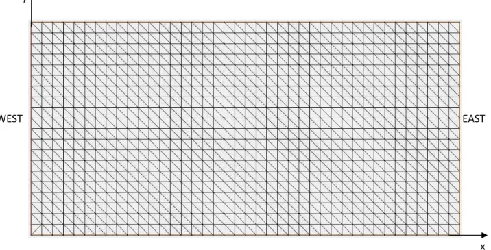
The test is carried out in an open channel with geometry: length L=80km, width B=40km (seen in Figure 1) and uniform still water depth h=20m. Tidal forcing is applied by prescribing semi- diurnal tidal elevations = %& '()! with %& = 1 at x=0 (western boundary) and the radiation boundary condition is applied at x=L=80km (eastern boundary). A constant bottom friction factor *+ = 0.01 is used in the test.
The following parameters are used in this test: grid size of -# = -. = 20 , time step of -! = 12 , horizontal eddy viscosity is computed by the closure model, Coriolis force is neglected and the model is run in the 2-D Barotropic mode.
3
Figure 1 Computational domain
Figure 2 Implementation of OBCs at the eastern boundary (a) Radiation OBC at all nodes; (b) Radiation OBC at interior nodes (red circle indicates the open boundary node)
x EAST WEST
(a) (b)
y
4
When setting up the model for the first time with the mesh layout in Figure 1, the radiation open boundary condition was applied to all nodes on the eastern boundary (seen in Figure 2a) and an error message related to the mesh layout at the north-east (NE) corner was received. This is because the mesh at the NE corner (seen in Figure 2a) has one open boundary side and one solid boundary side. To avoid this problem, we simply neglect both corner nodes when specifying radiation open boundary conditions, i.e. applying the radiation boundary condition at only interior nodes of the down-stream open boundary (eastern boundary in Figure 2b).
3. Exact Numerical Solution
Due to nonlinearity caused by the surface elevation, the advection and the nonlinear bottom friction, it is not possible to obtain an analytical solution with which we can validate the effectiveness of the radiation boundary condition. However, it is possible to obtain an exact (no- reflection) numerical solution by running the model in a very long channel and stopping the run before any reflected wave reach the test area, the western 80km portion of the channel in this case. As the phase speed is ≈ ℎ = 29.81 × 20 / ≈ 50km/hour, we choose the length of channel L=3000km which assures no reflection reaching x<80km within about 120 hours. The time step for this long channel case is 12s and the model run is stopped at t=60hours. No ramp- up of the specified surface elevation at x=0 was employed, since = %& '()! starts at = 0 at t=0.
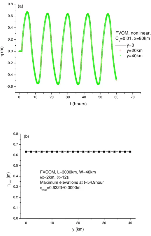
The amplitudes of tidal elevation and velocity at any node are computed by %(#) = ( 45 − 678)/2 and 9(#) = (945 − 9678)/2. The amplitudes along the central line of the entire channel and in the first 80km portion are plotted in Figure 3. The results in the first 80km portion will be adopted as the exact solution to validate the radiation boundary conditions in FVCOM. The time series of surface elevations at y=0, 20km, 40km for the cross section located at x=80km are shown in Figure 4a. It can be seen that a periodic state is obtained after about 10 hours and that a uniform condition is obtained in the cross-channel direction as the series at the three locations are exactly the same. More clearly, the variation of elevations in the cross- channel direction can be seen in Figure 4b, in which the maximum elevations for all nodes at
5
x=80km and at time t=54.9 hours are plotted. The results suggest that at maximum the elevations in the cross section at x=80km are exactly the same up to 4 digits, i.e. 45 = 0.6323 for all 21 nodes in this cross section. This means that the elevations in the cross-channel direction are uniform.
0 500 1000 1500 2000 2500 3000
0.0 0.2 0.4 0.6 0.8 1.0
0 10 20 30 40 50 60 70 80
0.3 0.4 0.5 0.6 0.7 0.8 0.9 1.0
Amplitude
x (km)
FVOM, nonlinear, Cb=0.01,L=3000km Ele. (m) Vel. (m/s)
Amp.
x (km) For x<80km
Figure 3 Exact numerical solution of elevation and velocity amplitudes along the central line of the long channel
6
0 10 20 30 40 50 60 70
-0.6 -0.4 -0.2 0.0 0.2 0.4 0.6 0.8
η (m)
t (hours)
FVOM, nonlinear, Cb=0.01, x=80km
y=0 y=20km y=40km (a)
0 10 20 30 40
0.0 0.1 0.2 0.3 0.4 0.5 0.6 0.7 0.8
η max (m)
y (km) FVCOM, L=3000km, W=40km δx=2km, δt=12s
Maximum elevations at t=54.9hour ηmax=0.6323±0.0000m
(b)
Figure 4 Surface elevations at x=80km of 3000km long channel. (a) Time series of surface elevation at three locations on the eastern boundary; (b) Maximum elevation across channel
width at t=54.9 hours
7
4. Simulation in a L=80km Long Channel
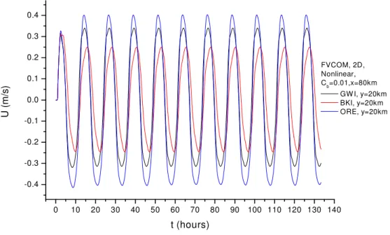
FVCOM is first run by specifying radiation OBC at only interior nodes of the eastern boundary (seen in Figure 2b). Three radiation boundary conditions, GWI, BKI and ORE, are applied in this calculation. The amplitudes of surface elevation and velocity along the central line of the channel are plotted together with the exact numerical solution in Figure 5a and Figure 5b, respectively. These results clearly show that none of the three radiation boundary conditions give the desired result of not causing any reflection. As seen in Figure 5a, the amplitude at the east boundary computed with GWI and ORE is about 1.1m, which is about 80% larger than the “exact” solution of 0.60m. If interpreted in a “linear” fashion, this means that GWI and ORE generate ≈ 80% reflection at the boundary. The result obtained with BKI is better than GWI and ORE, but still has about 40% reflection. Time series of elevation and velocity for the three types of radiation OBCs at the mid-point of the eastern boundary are shown in Figure 6a and 6b. The results in Figure 6a and 6b suggest that the periodic state has been achieved after about 10 hours for all the three cases. Analysis of the elevation amplitudes at all 21 nodes on the eastern boundary reveals that the means and derivations are 1.079 ± 0.001 , 0.693. ±0.006 and 1.091 ± 0.001 for GWI, BKI and ORE, respectively. This means the numerical solutions are almost uniform in the cross-channel direction.
0 10 20 30 40 50 60 70 80
0.6 0.7 0.8 0.9 1.0 1.1 1.2 (a)
Ele. Amp. (m)
x (km) FVCOM, 2D mode
Nonlinear friction, Cb=0.01 Exact Num. GW I BKI ORE
8
0 10 20 30 40 50 60 70 80
0.0 0.1 0.2 0.3 0.4 0.5 0.6 0.7
FVC OM, 2D m ode N onlinear friction, Cb=0.01
Exact N um . GW I BKI OR E
x (km )
Vel. Amp. (m/s)
(b)
Figure 5 Amplitudes along the central line of the channel for various OBCs, (a) Surface elevation; (b) Depth-averaged velocity.
0 10 20 30 40 50 60 70 80 90 100 110 120 130 140 -1.0
-0.5 0.0 0.5 1.0
FVCOM, 2D, Nonlinear, Cb=0.01,x=80km
GW I, y=20km BKI, y=20km ORE, y=20km
t (hours)
η (m)
9
0 10 20 30 40 50 60 70 80 90 100 110 120 130 140 -0.4
-0.3 -0.2 -0.1 0.0 0.1 0.2 0.3 0.4
FVCOM, 2D, Nonlinear, Cb=0.01,x=80km
GW I, y=20km BKI, y=20km ORE, y=20km
U (m/s)
t (hours)
Figure 6 Time series at three locations on the eastern boundary for various OBCs, (a) Surface elevations; (b) Depth-averaged velocity
In FVCOM, a sponge layer is optional for the open boundary treatment, which works together with other OBCs. Two parameters, the influence radius > and the damping coefficient
? , need to be specified to apply a sponge layer. Here we make a simple test by specifying
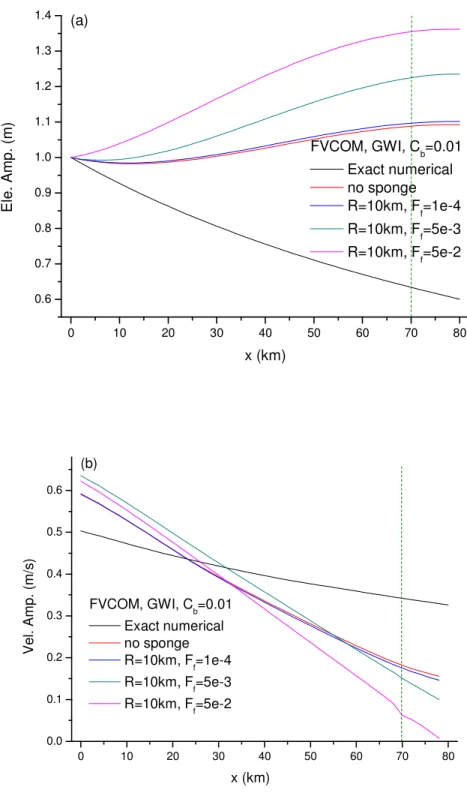
> = 100 and three values of ? =0.0001, 0.005 and 0.05 to check if the inclusion of a sponge layer helps to reduce boundary reflection. The GWI condition is selected to work together with the sponge layer. The computed amplitudes for the three types of sponge layer conditions are plotted with the exact numerical solution obtained in the long channel and also the solution without sponge layer for surface elevation and velocity in Figure 7a and 7b, respectively. It needs to be noted that the comparisons should be limited to # ≤ 700 (in the portion left of the dashed line in Figure 7a and 7b) as the last 10km portion is in the sponge layer.
The results in Figure 7a and 7b clearly show that the incorporation of a sponge layer makes the results worse. Actually, larger reflections are obtained for a larger damping coefficient for both surface elevation in Figure 7a and velocity in Figure 7b.
10
0 10 20 30 40 50 60 70 80
0.6 0.7 0.8 0.9 1.0 1.1 1.2 1.3 1.4
FVCOM, GWI, Cb=0.01 Exact numerical no sponge R=10km, Ff=1e-4 R=10km, Ff=5e-3 R=10km, Ff=5e-2
Ele. Amp. (m)
x (km) (a)
0 10 20 30 40 50 60 70 80
0.0 0.1 0.2 0.3 0.4 0.5 0.6
x (km)
Vel. Amp. (m/s)
FVCOM, GWI, C
b=0.01
Exact numerical no sponge R=10km, F
f=1e-4
R=10km, F
f=5e-3
R=10km, Ff=5e-2 (b)
Figure 7 Amplitudes with sponge layers, (a) Surface elevations; (b) Depth-averaged velocity
11
5. Identification and Correction of Implementation Error in FVCOM’s Radiation OBCs
As discussed in Section 4, very strong reflections are generated by the radiation open boundary conditions (OBCs) in FVCOM, especially GWI and ORE as seen in Figure 5a. The results look unreasonable. Some additional tests (not shown here) with the Princeton Ocean Model (POM) and the exact same radiation OBCs provide much less reflections for the same test case. This indicates that some errors may exist in the implementation of radiation OBC in FVCOM. Examinations of the relevant codes in FVCOM reveal that the problem is caused by the inconsistency of numerical scheme of the time derivative term / ! for open boundary and interior nodes. In FVCOM, a modified 4th order Runge-Kutta time stepping scheme is used to do temporal integration for interior nodes. The radiation boundary condition is implemented within the 4-step Runge-Kutta procedure. Therefore, the correct numerical formulation for radiation condition (1) should read
AB = − CD-! E F G + H (2)
Where should be the elevation at the open boundary at the previous time step and CD is the factor coming with the Runge-Kutta method. The examination of the manner in which (2) is implemented in FVCOM reveals that, is taken as the value at the intermediate step within the Runge-Kutta procedure and CD is fixed at 1. The original and corrected programs for the implementation of the GWI and BKI open boundary conditions are presented in an Appendix.
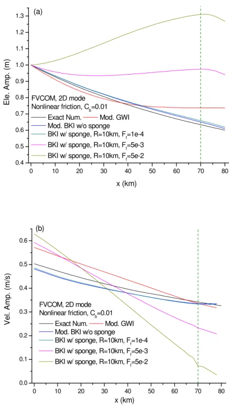
The amplitudes computed by FVCOM with corrected numerical formulation of GWI and BKI conditions are shown in Figure 8a and 8b for surface elevation and velocity, respectively. Apparently, the elevation amplitude in Figure 8a becomes much closer to the exact numerical solution than the original boundary condition (seen in Figure 5a), especially BKI yields excellent results. A sponge layer is also taken into account together with the BKI condition in this test. The radius of the sponge layer is fixed at 10km and damping coefficients are chosen as 0.0001, 0.005 and 0.05. The results shown in Figure 8a and Figure 8b suggest that the inclusion of a sponge layer make the predictions worse and the agreement with the exact numerical solution grows poorer the larger the damping coefficient. Again, the comparisons are limited to # ≤ 700 .
12
0 10 20 30 40 50 60 70 80
0.4 0.5 0.6 0.7 0.8 0.9 1.0 1.1 1.2 1.3
x (km)
Ele. Amp. (m)
FVCOM, 2D mode Nonlinear friction, C
b=0.01
Exact Num. Mod. GWI Mod. BKI w/o sponge
BKI w/ sponge, R=10km, Ff=1e-4 BKI w/ sponge, R=10km, Ff=5e-3 BKI w/ sponge, R=10km, F
f=5e-2
(a)
0 10 20 30 40 50 60 70 80
0.0 0.1 0.2 0.3 0.4 0.5 0.6
x (km)
Vel. Amp. (m/s)
FVCOM, 2D mode Nonlinear friction, C
b=0.01
Exact Num. Mod. GWI Mod. BKI w/o sponge
BKI w/ sponge, R=10km, Ff=1e-4 BKI w/ sponge, R=10km, F
f=5e-3
BKI w/ sponge, R=10km, Ff=5e-2 (b)
Figure 8 Amplitudes along the central line of the channel for corrected radiation open boundary conditions. (a) Surface elevations; (b) Depth-averaged velocity
13
6. Effect of mesh layout at corners
As mentioned in Section 2, the layout of meshes at the NE corner may cause problems in the implementation of radiation OBCs. From the error message, the open boundary condition cannot be specified at a node which is in a cell having one open boundary side and one solid boundary side or two open boundary sides. So we did not specify the radiation open boundary condition at the two corner nodes for the simulations in Section 3-5. The results in those sections show that this treatment works well.
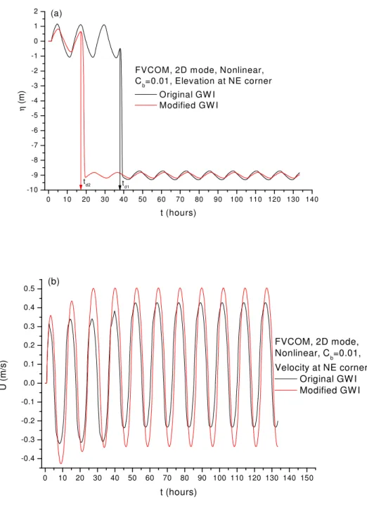
Alternatively, we may modify the NE corner cell in the original mesh (seen in Figure 2a or in Figure 9a) to the one show in Figure 9b to avoid one open boundary side and one solid boundary in the same cell, which is exactly the same as done in FVCOM test cases (see SW corner cell in Figure 2a). With this modification, no mesh error message is received, and FVCOM is run by applying the original and modified GWI radiation boundary condition including corners along the entire eastern boundary. The time series of elevation and velocity at the NE corner on the eastern boundary are plotted in Figure 10a and Figure 10b for both original and modified GWI conditions. Some strange results are obtained. As seen in Figure 10a, the elevations at the NE corner drop suddenly by about 9.3m at !I ≈ 38 hours for the original GWI and at !I ≈ 18 hours for the modified GWI. The velocity at the same point also changes after time !I (seen in Figure 10b), but by a much smaller amount (an increase of about 0.15 m/s).
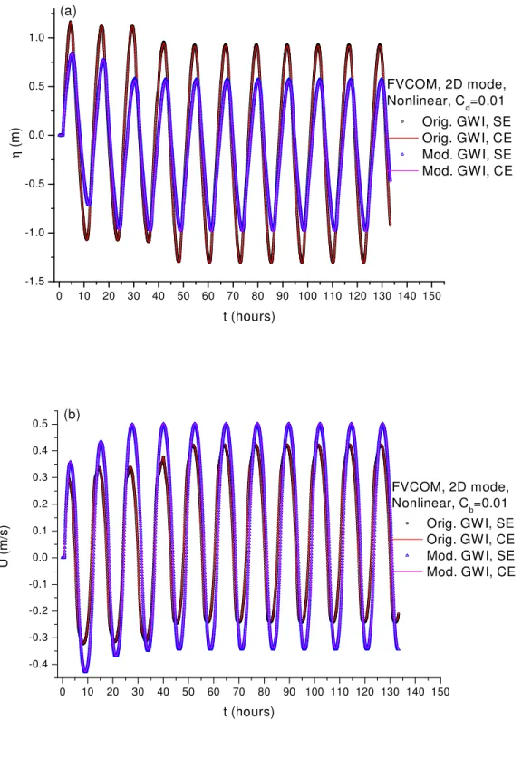
The time series of elevation and velocity at the other two boundary points, the lower corner (SE) and the center point (CE) on the eastern open boundary are plotted in Figure 11a and 11b, respectively. The results in Figure 11a show that the elevations at SE and CE points also have drops, but much smaller (about 0.15m) than that at the NE corner. The changes of velocity at the SE and CE points are similar to the velocity change at the NE corner, i.e. increasing by about 0.15m/s.
It can be seen from Figure 10a that a periodic state has been reached before the sudden drop for the case with the original GWI condition. Analysis of elevation time series for the original GWI condition before and after the sudden drop suggests that the amplitude changes very little after the sudden drop, from 1.098m to 1.113m. Both of them are quite close to the one (1.092m) obtained in section 4 for the case without the two corners on the eastern boundary included.
14
Figure 9 Layout of meshes at the northwest corner (a) original one; (b) modified one (red circle indicates the open boundary node)
An interesting thing is that no dramatic drop occurs at the SE corner although all input conditions are exactly the same at the SE and NE points. Further check suggests that the dramatic drop of elevation occurs also at several northern boundary nodes near the NE corner node and the drop magnitude decreases with increasing distance from the NE corner node along the northern boundary. The elevation drop magnitudes for the two types of GWI boundary conditions near the NE corner on the northern boundary are quite similar, which are about 9.3m, 9.3m, 1.7m, 0.8m, and 0.4m from the NE corner (from 1st to 5th node on the north boundary).
(a) (b)
15
0 10 20 30 40 50 60 70 80 90 100 110 120 130 140 -10
-9 -8 -7 -6 -5 -4 -3 -2 -1 0 1 2
η (m)
t (hours)
FVCOM, 2D m ode, Nonlinear, Cb=0.01, Elevation at NE corner
Original GW I Modified GW I (a)
td1 td2
0 10 20 30 40 50 60 70 80 90 100 110 120 130 140 150 -0.4
-0.3 -0.2 -0.1 0.0 0.1 0.2 0.3 0.4 0.5
FVCOM, 2D mode, Nonlinear, Cb=0.01, Velocity at NE corner
Original GW I Modified GW I
U (m/s)
t (hours) (b)
Figure 10 Time series at the NE corner for the case with NE corner node included, (a) Surface elevation; (b) Depth-averaged velocity.
16
0 10 20 30 40 50 60 70 80 90 100 110 120 130 140 150 -1.5
-1.0 -0.5 0.0 0.5 1.0
η (m)
FVCOM, 2D mode, Nonlinear, Cd=0.01 Orig. GW I, SE Orig. GW I, CE Mod. GWI, SE Mod. GWI, CE
t (hours) (a)
0 10 20 30 40 50 60 70 80 90 100 110 120 130 140 150 -0.4
-0.3 -0.2 -0.1 0.0 0.1 0.2 0.3 0.4 0.5
FVCOM, 2D mode, Nonlinear, C
b=0.01
Orig. GW I, SE Orig. GW I, CE Mod. GW I, SE Mod. GW I, CE
U (m/s)
t (hours) (b)
Figure 11 Time series at the SE and CE points for the case with NE corner node included, (a) Surface elevation; (b) Depth-averaged velocity.
17
7. Conclusion
An error in FVCOM’s radiation condition implementation has been identified and corrected. Results for the simple test case are quite good for the correct implementation of GWI and BKI boundary conditions, with BKI giving the better. Tests with a sponge layer included suggest that the incorporation of sponge layers does not help to reduce but actually increases reflection caused by GWI and BKI conditions at the open boundary.
For this simple test case all radiation boundary conditions can be expressed by Equation (1). The wave speed: = ℎ in (1) is constant for both GWI and BKI, and = and
= 3 ℎ are prescribed for GWI and BKI, respectively. The value of may play a key role in the radiation boundary condition. This could be the reason why BKI performs better than GWI. And the reason why BKI does not predict as good an agreement of velocity as surface amplitude (Figure 8a and 8b) could be the specification of an inaccurate value of , i.e. the best value of may not be 3 hours. We are currently attempting to develop a methodology for the prediction of approximate values for the two parameters, and , in the generalized radiation boundary condition (1).
A strange result was obtained when specifying a radiation OBC at the NE corner node by changing the mesh layout to be accepted by FVCOM. The elevation at the NE corner drops suddenly by about 9.3m while the model keeps running. We did not experience this problem when not designating the two corner points as open boundary points, but have no idea why this worked.
18
Appendix
As described in Section 5, the numerical implementation of the open boundary condition in FVCOM is wrong and has been corrected. Here we attach the relevant program for GWI condition to show how the correction is made.
FVCOM solves the time integration of elevation in subroutine “extel_gcn.F” with relevant lines given:
!---PERFORM UPDATE ON ELF---! DTK = ALPHA_RK(K)*DTE
ELF = ELRK - DTK*XFLUX/ART1
Where “ELRK “ is the elevation at the previous time step which is stored before carrying out Runge-Kutta integration and “ALPHA_RK(K)” isCD in equation (2) with values of ¼, 1/3, ½, and 1 for k=1, 2, 3 and 4, respectively. The parameter “K”, from 1 to 4, is the index of the Runge-Kutta procedure, which need to be passed from the main program “us_fvcom.F” to the subroutine which needs it. Thus, we can do the integration of open boundary condition (2) in the same way as that in “extel_gcn.F”. To have “K” in “Bcond_GWI.F”, the routines “Bcond_gcn.F”,
“Bcond_gcn.F” and “Bcond_GWI.F” should be modified to carrying this parameter.
Original code of Subroutine Bcond_GWI:
!====================================================================| SUBROUTINE BCOND_GWI
!---|
! GRAVITY-WAVE RADIATION IMPLICIT OPEN BOUNDARY CONDITION (GWI) |
!---| USE ALL_VARS
IMPLICIT NONE INTEGER :: I1,I2,J,JN REAL(SP):: CC,CP
DO J = 1,IBCN(3) JN = OBC_LST(3,J) I1 = I_OBC_N(JN) I2 = NEXT_OBC(JN)
CC = SQRT(GRAV*H(I1))*DTE/DLTN_OBC(JN) CP = CC + 1.0_SP
ELF(I1) = (CC*ELF(I2) + EL(I1))/CP END DO
RETURN
END SUBROUTINE BCOND_GWI
!===================================================================|
19 Corrected code of Subroutine Bcond_GWI:
!===================================================================| SUBROUTINE BCOND_GWI (K_RK)
!---|
! GRAVITY-WAVE RADIATION IMPLICIT OPEN BOUNDARY CONDITION (GWI) |
!---| USE ALL_VARS
IMPLICIT NONE INTEGER :: I1,I2,J,JN REAL(SP):: CC,CP
INTEGER :: K_RK ! ADD BY MAPEIFENG ON AUG 11, 2008
DO J = 1,IBCN(3) JN = OBC_LST(3,J) I1 = I_OBC_N(JN) I2 = NEXT_OBC(JN)
CC = SQRT(GRAV*H(I1))*DTE/DLTN_OBC(JN)*ALPHA_RK(K_RK) CP = CC + 1.0_SP
ELF(I1) = (CC*ELF(I2) + ELRK(I1))/CP END DO
RETURN
END SUBROUTINE BCOND_GWI
!==========================================================================|
Original code of Subroutine Bcond_BKI:
!==========================================================================| SUBROUTINE BCOND_BKI
!---|
! BLUMBERG AND KHANTA IMPLICIT OPEN BOUNDARY CONDITION |
!---|
USE ALL_VARS IMPLICIT NONE
INTEGER :: I1,I2,J,JN REAL(SP):: CC,CP
DO J = 1,IBCN(4) JN = OBC_LST(4,J) I1 = I_OBC_N(JN) I2 = NEXT_OBC(JN)
CC = SQRT(GRAV*H(I1))*DTE/DLTN_OBC(JN) CP = CC + 1.0_SP
ELF(I1) = (CC*ELF(I2) + EL(I1)*(1.0_SP-DTE/10800.0_SP))/CP END DO
RETURN
END SUBROUTINE BCOND_BKI
!============================================================================|
20 Corrected code of Subroutine Bcond_BKI:
!==========================================================================| SUBROUTINE BCOND_BKI (K_RK)
!---|
! BLUMBERG AND KHANTA IMPLICIT OPEN BOUNDARY CONDITION |
!---|
USE ALL_VARS IMPLICIT NONE
INTEGER :: I1,I2,J,JN REAL(SP):: CC,CP
DO J = 1,IBCN(4) JN = OBC_LST(4,J) I1 = I_OBC_N(JN) I2 = NEXT_OBC(JN)
CC = SQRT(GRAV*H(I1))*DTE/DLTN_OBC(JN)*ALPHA_RK(K_RK) CP = CC + 1.0_SP
ELF(I1) = (CC*ELF(I2) + ELRK(I1)*(1.0_SP-DTE/10800.0_SP))/CP END DO
RETURN
END SUBROUTINE BCOND_BKI
!============================================================================|