Game5 最近の更新履歴 yyasuda's website

In part two of this book, we have looked at the extreme market structures of monopoly and perfect competition. Although these are useful points of reference, empirical observation suggests that most real-world markets are somewhere between the extremes. Normally, we ind industries with a few (more than one) irms, but less than the "very large number" usually assumed by the model of perfect competition. The situation in which there are a few competitors is deSignated by oligopoly (duopoly if the number is two).

One thing the extremes of monopoly and perfect competition have in common is that each irm does not have to worry about its rivals' reactions. In the case of monopoly, this is trivial as there are no rivals. In the case of perfect competition, the idea is that each irm is so small that its actions have no signiicant impact on rivals. Not so in the case of oligopoly. Consider the follOWing news article excerpt:

In a strategic shit in the United States and Canada, Coca-Cola Co. is .. . gearing up to raise the prices it charges its customers for sot drinks byabout 5% ^.. . The price changes could help boost Coke's profit . . .

Important to the success of Coke and its bottlers is how Pepsi-Cola . . '. responds. The NO.2 sot-drink company could well sacriice some margins to pick up market share on Coke, some analysts said.n

As this example suggests, by contrast with the extremes of monopoly and perfect competition, an important characteristic of oligopolies is the strategic interdependence between competitors: An action by Firm 1, say, Coke, is likely to inluence Firm 2's proits, say, Pepsi, and vice versa. For this reason, Coke's decision process should take into account what it expects Pepsi to do, speciically, how Coke expects its decisions to impact on Pepsi's proits and, consequently, how it expects Pepsi to react. Part three

P TE R ₇

102

_I

^{PART3 CHAPTER 7}

• Moreover, in a dynamic setting, Compaq must also take inlo account that current price choices will likely inluence the rival's future price choices. This we will see in chapter 8,

b The Bertrand model is more general than the simpliied v�^rsion

presented here, but the main ideas are the same.

'What does "just below" mean? If p, could be any real number, then "just below" w�uld not be well deined: There exists no real number "just below" another real number, In practice, prices have ¹⁰ be set on a inil! grid (in cents aftha dollar. for example), in which case

"just below" would mean one ccnt loss. This points to an important assumption of the Berlrand model: Firm 1 will steal all of Firm 2'$' demand even If its price is only one cent lower than the rival's,

of this book is dedicated to the formal analysis of oligopoly competition. We ^{begin in} this chapter with some simple models that characterize the process of interdependent strategic decision making under oligopoly: the Bertrand model and the Cournot model.

7.1 THE BERTRAND MODEL

Pricing is probably the most basic strategy that irms must decide on. The demand received by each irm depends on the price it sets. Moreover, when the number ^of irms is small, demand also depends on the prices set by rival irms. It is ^precisely this interdependence between rivals' decisions that differentiates duopoly competition (and more generally oligopoly competition) rom the extremes of ,monopoly and perfect

,competition. When Compaq, for example, decides which prices to set for its PCs^{, the}

company has to make some conjecture regarding the prices set by rival Dell. ^{Based on} this conjecture it must determine the optimal price, taking into account how demand ^for the Compaq PC depends on both the Compaq price and the Dell price. ^a

To analyze the interdependence of pricing decisions, we begin with the simplest model of duopoly competition, the Bertrand mode\.73 The model consists of two irms in a market for a homogeneous product and the assumption that irms simultaneously set their prices. We will also assume that both irms have the same marginal cost, MG, that marginal cost is constant, and that the demand is linear.b

Because the duopolists' products are perfect substitutes (the product is homoge- neous), whichever irm sets the lowest price gets all of the demand. Speciically, ^{if Pi,} the price set by irm j, is ldwer than ^Pj' the price set by irm ^j, then irm j's demand is given by D(Pi) (the market demand). whereas irm ^j's demand is zero. If both irms set the same price, Pi ⁼ Pj ^{= P,} then each irm receives one half of the market demand, ^{! D(p).}

What is each irm's best strategy in this context? As suggested previously, Firm ^l's optimal price depends on what it conjectures Firm 2 will choose, and vice versa. Suppose that Firm 1 expects Firm 2 to price above monopoly price. Then Firm l's optimal ^strategy is to price at the monopoly level. In fact, by doing so, Firm 1 gets all of the demand ^and receives monopoly profits (the maximum possible proits). If Firm 1 expects Firm ^{2 to} price below monopoly price but above marginal cost, then Firm l's optimal strategy is to set a price just below that of Firm 20 Pricing above would lead to zero demand and zero proits. Pricing below gives irm j all of the market demand, but with lower proits^{, the} lower the price is. Finally, if Firm 1 expects Firm 2 to price below marginal cost, then Firm l's optimal choice is to price higher than Firm 2, say, at marginal cost level.

The preceding set of optimal prices deines Firm l's best response with respect to Firm 2's choice. More generally, irm i's ^{best response} (also known as reaction unction)

is a function ^pj(pj) that gives, for each price by irm ^j, firm j's optimal price.

PI

pM

� � h

/

^{h I}

,/

^I

/ /

45°

pi(P2)

MC I <'

/

k

^{/ /}

/ _I

MC pM ^{) P2}

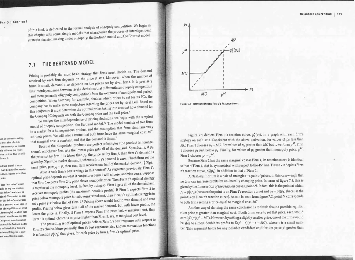
FIGURE _7.1 BERTRAND MO'DEL: FIRM _l's REACTION CURVE.

Figure 7.1 depicts Firm l's reaction curve, p�(P2)' in a graph with each irm's strategy on each axis. Consistent with the above derivation, for values of ^P2 less than MG, Firm 1 chooses Pl = MG. For values of P2 greater than MG but lower than pM, Firm 1 chooses Pl just below P2' Finally, for values of P2 greater than monopoly price, pM, Firm 1 chooses Pl ⁼ pM.

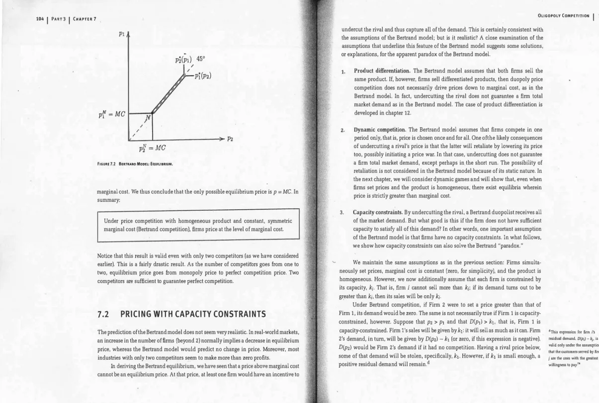
Because Firm 2 has the same marginal cost as Firm 1, its reaction curve is identical to that of Firm 1, that is, symmetrical with respect to the

_45°

line. Figure 7.2 depicts Firm 2's reaction curve, pi(Pl), in addition to that of Firm 1.

A Nash equilibrium is a pair of strategies-a pair of prices, in this case-such that no irm can increase proits by unilaterally changing price. In terms of igure 7.2, this is given by the

intersect jon of the reaction curves,

point N. In fact, this is the point at which Pl ⁼ pj(P2) (because the point is on Firm l's reaction curve) and P2 ⁼ pi(Pl) (because the point is on Firm 2's reaction curve). As can be seen rom igure 7.2, point N corresponds to both irms setting a price equal to marginal cost, MG.

Another way of deriving the same conclusion is to think about a possible equilib-^, rium price p' greater than marginal cost. If both irms were to set that price, each would earn � D(p')(p' ^-MG). However, by setting a slightly smaller price, one of the irms would be able to almost double its proits to D(p' - E)(p' ^{-E -}MG), where ^E is a small num­ ber. This argument holds for any possible candidate equilibrium price p' greater than

104

_I

^{PART 3}

_I

^CHAPTER 7

PI

PI

N ⁼

^{MC I}

^__

^'

� �. /

P2(Pl)

^45°

1/ pi(P2)

k

>

_P2

P� ^=MC

FIGURE 7.2 BERTRAND MODEl: E.UILIBRIUM.

marginal cost. We thus conclude that the only possible equilibrium price is p ⁼ MG. In summary:

Under price competition with homogeneous product and constant, symmetric marginal cost (Bertrand competition), irms price at the level of marginal cost.

Notice that this result is valid even with only two competitors (as we have considered earlier). This is a fairly drastic result. As the number of competirors goes rom one to two, equilibrium price goes rom monopoly price to perfect competition price. Two competitors are suficient to guarantee perfect competition.

7.2 PRICING WITH CAPACITY CONSTRAINTS

The prediction of the Bertrand model does not seem very realistic. In real-world markets, an increase in the number of irms (beyond 2) normally implies a decrease in equilibrium price, whereas the Bertrand model would predict no change in price. Moreover, most industries with only two competitors seem to make more than zero proits.

In deriving the Bertrand equilibrium, we have seen that a price above marginal cost cannot be an equilibrium price. At that price, at least one irm would have an incentive to

OLIGOPOLY COMPETITION

I

¹⁰⁵

undercut the rival and thus capture all of the demand. This is certainly consistent with the assumptions of the Bertrand model; but is it realistic? A close examination of the assumptions that underline this feature of the Bertrand model suggests some solutions, or explanations, for the apparent paradox of the Bertrand model.

1. Product diferentiation. The Bertrand model assumes that both irms sell the same product. If, however, irms sell differentiated products, then duopoly price competition does not necessarily drive prices down to marginal cost, as in the Bertrand model. In fact, undercutting the rival does not guarantee a irm total market demand as in the Bertrand model. The case of product differentiation is developed in chapter 12.

2. Dynamic competition. The Bertrand model assumes that irms compete in one period only, that is, price is chosen once and for all. One ofthe likely consequences of undercutting a rival's price is that the latter will retaliate by lowering its price too, possibly initiating a price war. In that case, undercutting does not guarantee a irm total market demand, except perhaps in the short run. The possibility of retaliation is not considered in the Bertrand model because of its static nature. In the next chapter, we will consider dynamic games and will show that, even when irms set prices and the product is homogeneous, there exist equilibria wherein price is strictly greater than marginal cost.

3. Capacity constraints. By undercutting the rival, a Bertrand duopolist receives all of the market demand. But what good is this if the irm does not have suicient capacity to satisy all of this demand? In other words, one important assumption of the Bertran� model is that irms have. no capacity constraints. In what follows, we show how capacity constraints can also solve the 'Bertrand "paradox."

We maintain the same assumptions as in the previous section: Firms simulta­ neously set prices, marginal cost is constant (zero, for simplicity), and the product is homogeneous. However, we now additionally assume that each irm is constrained by its capacity, kj• That is, irm j cannot sell more than kj; if its demand turns out to be greater than k;, then its sales will be only kj.

Under Bertrand competition, if Firm 2 were to set a price greater than that of Firm 1, its demand would be zero. The same is not necessarily true if Firm 1 is capacity­ constrained, however. Suppose that pz > _PI and that D(PI) ^> kl, that is, Firm 1 is capacity-constrained, Firm l's sales will be given by kl: it will sell as much as it can. Firm 2's demand, in turn, will be given by D(pz) ^-ki (or zero, if this expression is negative). D(pz) would be Firm 2's demand if it had no competition. Having a rival price below, some of that demand will be stolen, speciically, ki. However, if ki 'is small enough, a positive residual demand will remaind

dThis expression for irm j's residual demand. D{Pi) -k;. is valid only under the assumption that the customers served by inn j are the ones with the greatest willingness to pay,14

I I

• D(p), the direct demand curve (or simply demand curve), corresponds to taking price as the independent variable, thaI is, quantity as a function of price; P(Q), the inverse demand curve, corresponds to laking quantity as the independent variable. that is, price as a function or quantity .

FIGURE 7.3 FIRM 2's OPTIMUM.

The situation of price competition (Bertrand competition) with capacity constraints is illustrated in igure 7.3. _D(p) is the demand curve. Two vertical lines represent each irm's capacity. In this example, Firm 2 is the one with greater capacity: k2 > k1. The third vertical line, kl + k2' represents total industry capacity.

Let P(Q) be the inverse demand curve, that is, the inverse of D(p).-Moreover, let P(k1 + k2) be the price level such that, if both irms were to set p = P(k1 + k2), total demand would be exactly equal to total capacity. This price level is simply derived from the intersection of the demand curve with the total capacity curve. We will now argue that the equilibrium of the price-setting game consists of both irms setting _Pi ⁼ P(kt + k2). In other words, irms set prices such that total demand equals industry capacity.

Let us consider Firm 2's optimization problem assuming that Firm 1 sets _Pl =

P(k1 + k2). Can Firm 2 do better than setting P2 = Pl = P(k1 + i2)? One alternative strategy is to set P2 ^< P(k1 + k2). By undercutting its rival, Firm 2 receives all of the market demand. However, because Firm 2 is already capacity-constrained when it sets P2 = P(k1 + k2), setting a lower price does not help: On the contrary, Firm 2 receives lower profits by setting a lower price (same output sold at a lower price).

What about setting a price higher than P(k1 + k2)? The idea is that, because Firm 1 is capacity-constrained when Pl = P(k1 + k2l. Firm 2 will receive positive demand even if it prices above Firm 1. Figure 7.3 depicts Firm 2's residual demand, d2, under the assumption that P2 > Pl and Pl = P(k1 + k2): Firm 2 gets D(p21. minus Firm 1 's output, kl' so d2 is parallel to D, the difference being k1. The igure also depicts Firm 2's marginal revenue curve, r2. As can be seen, marginal revenue is greater than marginal cost (zero) for every value of output less than Firm 2's capacity. This implies that setting a higher

I

price than P(k1 + k2), which is the same as selling a lower output than q2 = k2' would imply � lower proit: The revenue loss (the positive marginal revenue) is greater than the cost saving (the value of marginal cost, which is zero).

A similar argument would hold for Firm 1 as well: Given that P2 ⁼ P(k1 + k2), Firm 1 's optimal strategy is to set Pl ⁼ P(k1 + k2). We thus conclude that Pl ⁼ P2 = P(k1 + k2) is indeed an equilibrium. Notice that, if capacity levels were high, then the previous argument would not hold; that is, it might be optimal for a irm to undercut its rival's price. However, if capacities are relatively small, then the result obtains that equilibrium prices are such that total demand equals total capacityJ In summary:

If total industry capacity is low in relation to market demand, then equilibrium prices are greater than marginal cost.

To conclude, notice that the same analysis applies to the case when irms must decide beforehand how much to produce and then set prices. In this case, each irm's sales are equal to the minimum of that irm's demand and its output. As a result, if total quantity produced is low relative to total demand, then in equilibrium, irms set prices such that total demand just clears the total output previously produced. That is, for each pair of output choices (ql, q2), equilibrium prices are given by Pl = P2 = P(ql + q2).

7.3 THE COURNOT MODEl

In the previous section we concluded that, if irms' sales are limited by the output they produced beforehand, then in equilibrium, firms set prices such that total demand just clears total output.s This analysis can be taken one step back: What output levels should irms choose in the irst place? Suppose that output decisions are made simultaneously before prices are chosen. Based on this analysis, irms know that, for each pair of output choices (ql, q2), equilibrium prices will be Pl = P2 = P(ql + q2). This implies that irm i's proit is given by fj =qi

₍

P(ql + q2) - c

₎

, assuming, as before, constant marginal cost, c. The game wherein irms simultaneously choose output levels is known as the Cournot model. 76 Speciically, suppose there are two firms in a market for a homogeneous product. Firms choose simultaneously the quantity they want to produce. The market price is then set at the level such that demand equals the total quantity produced by both irms.

As in section 7.1, our goal is to derive the equilibrium of the model, that is, the equilibrium of the game played between the two irms. Also as in section 7.1, we do so in two steps. First, we derive each irm's optimal choice given its conjecture of what the

rrr capacity costs are suficiently high. then irms' capacity levels will surely be sufiCiently low such that the previous result holds. However, it can be shown thai, even if capacity costs were low, the same would be true.1S

G The same applies for the cboice of production capacity. However, for the purpose of this section, we focus on the case when irms choose output level in the irst place.

. - .. - --,---. - -�- ^.

^{. -}

'

_,

'

_{. . . . . ., -}

108

_I

_{PART 3}

_I

CHAPTER ₇

hThis results from our assumption that domand is linear. In general, the marginal ravenue curve has the same intercept as the demand curve and a higher slope (in absolute value). not necessarily twice,the slope of the demand curve.

p

P(q2)

P(q�

⁺

q2) T Y

^-

_{, ,}

q2

fiGURE 7.4 FIRM l's OPTIMUM.

c

ql, q2

rival does, that is, the irm's reaction curve. Second, we put the reaction curves together and ind a mutually consistent combination of actions and conjectures.

Suppose that Firm 1 believes Firm 2 is producing a quantity q2· What is Firm l's optimal quantity? The answer is provided by igure 7.4. If Firm 1 decides not' to produce anything, then price is given by P(O + q2) ⁼ P(Q2). If Firm 1 instead

_p

roduces, say, q;, then price'is given by _P(q; + q2). More generally, for each quantity that Firm 1 might decide to set, price is given by the curve _dj(q2). The curve _dj(Q2) is called Firm l's residual demand: It gives all possible combinations of Firm l's quantity and price for a given a value of _q2'

Having derived Firm l's residual demand, the task of inding Firm l's optimum is now similar to inding the optimum under monopoly, which we have already done in chapter 5. Basically, we must determine the point at which marginal revenue equals marginal cnst. Marginal cost is constant by assumption and equal to c. Marginal revenue is a curve with twice the slope of _dj(qz) and with the same vertical intercept.h The point at which the two curves intersect corresponds to quantity qj(qz).

Notice that Firm l's optimum, qj(qz), depends on its belief about what Firm 2 is doin.. To ind an equilibrium, we are interested in deriving Firm l's optimum for other possible values of qz. Figure 7.5 considers two other possible values of qz· If q2 ^{= 0,} then Firm 1 's residual demand is effectively the market demand: d1

(0)

⁼ D. The optimal solution, not surprisingly, is for Firm 1 to choose the monopoly quantity; qj(O) ⁼ qM, where _qM is the monopoly quantity. If Firm 2 were to choose the quantity corresponding to perfect competition, that is qz ⁼ qC, where qC is such that P(qc) = c, then Firm l's

Q^'L1GOPOlY COMPETITION

I

¹⁰⁹

P

c

ql, q2

qj(qC) qj(O)

⁼

qM _qC

fiGURE 7.5 Two EXTREME CASES.

ql

qM

qC q2

FIGURE 7.6 FIRM l's REACTION FUNCTION.

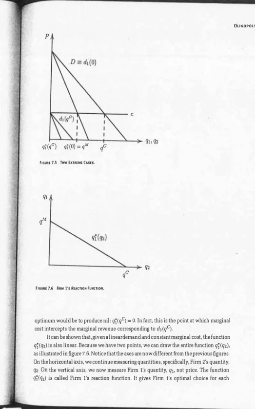
optimum would be to produce nil: qj(qC) ⁼ O. In fact, this is the point at which marginal cost intercepts the marginal revenue corresponding to _{d1 (qC).}

It can be shown that, given a linear demand and constant marginal cost, the function qj(qz) is also linear. Because we have two points, we can draw ilie entire function _qj(qz), as illustrated in igure 7.6. Notice iliat ilie axes are now different rom the previous igures. On the horizontal xis, we continue measuring quantities, speciically, Firm 2's quantity, qz. On the vertical axis, we now measure Firm l's quantity, _ql, not price. The function qj(qz) is called Firm l's reaction function. It gives Firm l's optimal choice for each

'The equilibrium concepl we Bre using here Is thai of Nash equilibrium. or NashCournot equilibrium, thus the n�lation N. In general, more than one equilibrium can exist. However, when the demand curve is linear and marginal cost Is constant, there exists only one equilibrium.

possible choice by Firm 2. Or, to look at it from a different perspective: It gives Firm l's choice given what it believes Firm 2 is choosing.

Throughout this chapter, in parallel with the graphical derivation of equilibria, we present the correponding algebraic derivation. Except for some results in the next section, algebra is not necessary for the derivation of the main results; but it may help, especially if the reader is familiar with basic algebra and calculus. Let us start with the algebraic derivation of Firm l's reaction function. Suppose that (inverse) demand is given by P(Q) ^{= a -bQ,} whereas cost is given by C(q) = cq, where q is the irm's output and Q = ql + qz is total output.

Firm l's proit is

fl =Pql - C(ql)

₌

(a -b(ql + qz)) ql - Cql·

The irst-order condition for the maximization Of]fl with respect to ql, afl/aql ⁼

0,

^is

-bql +a-b(ql +q2) - c =O, or simply

0-C q2

ql=�-2'

Because this gives the optimum ql for each value of q2, we have just derived the Firm l's reaction function, qt(q2):

(7.1)

We are now ready for the last step in our analysis, that of inding the equilibrium. An equilibrium is a point at which irms choose optimal quantities given what they conjecture the other irm is doing; and those conjectures are correct. Speciically, an equilibrium correspond to a pair of values (qlo q2) ^. such that ql is Firm l's optimal response given q2 and, likewise, q2 is Firm 2's optimal response given _ql· We have not derived Firm 2's reaction function. However, given our assumption that both irms have the same cost function, we conclude that Firm 2's reaction function, _qi(ql), is the symmetric of Firm l's. We can thus proceed to plot the two reaction functions on the same graph, as in igure 7.7.

The equilibrium point in the Cournot model is then given by the intersection of the reaction curves, point N. In fact, this is the point at which ql = qt(q2) (because the point is on Firm l's reaction curve) and q2 = qi(ql) (because the point is on Firm 2's reaction curveJ,i

I

qf

FIGUR'7.7 (OURNOT EQUILIBRIUM.

We now proceed with our algebraic derivation. In equilibrium, it must be that Firm 1 chooses an output that is optimal given what it expects Firm 2's output to be. If Firm 1 expects Firm 2 to produce q�, then it must be qf = qr(q�). Moreover, in equilibrium Firm l's conjecture regarding Firm 2's choice should be correct: _{q� = qf.} Together, these conditions imply that qf = qr(qf). The same conditions apply for Firm 2, that is, in equilibrium it must also be the case that qf = qi(qf). An equilibrium is thus deined by the system of equations

qf = qt(qf) qf =qi(qf)·

Equation (7.1) gives Firm l's reaction function. We can thus write the irst equation of the preceding system as

N ^{Q- c} qf

ql

_=;-"

Because the two irms are identical (same cost function), the equilibrium will also be symmetric, that is, _{qf = qf} = _qN. We thus have

N ^{Q -c qN} q

_=-b-T

Solving for qN, this yields

112

I

^PART3

I

^{CHAPTER 7}

MONOPOLY, DUOPOLY, AND PERFECT COMPETITION

Duopoly is an intermediate market structure, between monopoly (maximum concen­ tration of market shares) and perfect competition (minimum concentration of market shares). One would expect equilibrium price and output under duopoly also to lie be­ tween the extremes of monopoly and perfect competition.

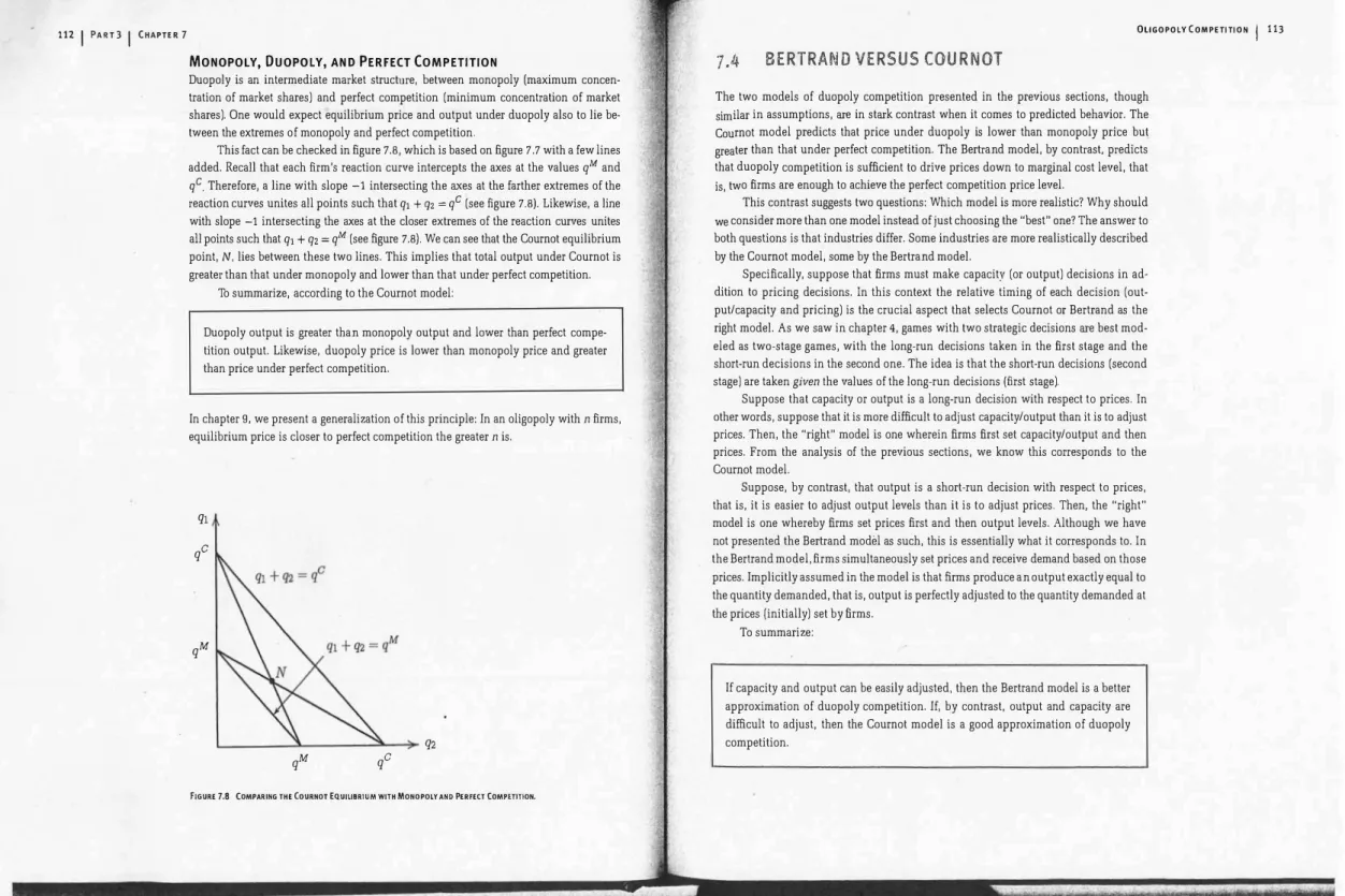
This fact can be checked in igure 7.8, which is based on igure 7.7 with a few lines added. Recall that each irm's reaction curve intercepts the axes at the values qM and qC Therefore, a line with slope -1 intersecting the axes at the farther extremes of the reaction curves unites all points such that ql + q2 ⁼ qC (see igure ^7.8). Likewise, a line with slope -1 intersecting the axes at the closer extreme's of the reaction curves unites all points such that ql + q2 ⁼ qM (see igure ^7.8). We can see that the Coumot equilibrium point,

_N,

lies between these two lines. This implies that total output under Coumot is greater than that under monopoly and lower than that under perfect competition.

To summarize, according to the Coumot model:

Duopoly output is greater than monopoly output and lower than perfect compe­ tition output. Likewise, duopoly price is lower than monopoly price and greater than price under perfect competition.

In chapter g, we present a generalization of this principle: In an oligopoly with ⁿ irms, equilibrium price is closer to perfect competition the greater n is.

ql qC

qM

qM qC q2

FIGURE 7.8 COMPARING THE (OURNOT EQUILIBRIUM WITH MONOPOLY AND PERfECT COMPETITION.

OLIGOPOLY COMPETITION

_I

113

7.4 BERTRAND VERSUS COURNOT

The two models of duopoly competition presented in the previous sections, though similar in assumptions, re in strk contrast when it comes to predicted behavior. The Coumot model predicts that price under duopoly is lower than monopoly price but greater than that under perfect competition. The Bertrand model, by contrast, predicts that duopoly competition is suicient to drive prices down to marginal cost level, that is, two irms are enough to achieve the perfect competition price level.

This contrast suggests two questions: Which model is more realistic? Why should we consider more than one model instead of just choosing the "best" one? The answer to both questions is that industries differ. Some industries are more realistically described by the Coumot model, some by the Bertrand model.

Speciically, suppose that irms must make capacity (or output) decisions in ad­ dition to pricing decisions. In this context the relative timing of each decision (out­ put/capacity and pricing) is the crucial aspect that selects Coumot or Bertrand as the right model. As we saw in chapter 4, games with two strategic decisions re best mod­ eled as two-stage games, with the long-run decisions taken in the irst stage and the short-run decisions in the second one. The idea is that the short-run decisions (second stage) are taken given the values of the long-run decisions (first stage).

Suppose that capacity or output is a long-run decision with respect to prices. In other words, suppose that it is more diicult to adjust capacity/output than it is to adjust prices. Then, the "right" model is one wherein irms irst set capacity/output and then prices. From the analysis of the previous sections, we know this corresponds to the Coumot model.

Suppose, by contrast, that output is a short-run decision with respect to prices, that is, it is easier to adjust output levels than it is to adjust prices. Then, the "right" model is one whereby irms set prices irst and then output levels. Although we have not presented the Bertrand model as such, this is essentially what it corresponds to. In the Bertrand model. irms Simultaneously set prices and receive demand based on those prices. Implicitly assumed in the model is that irms produce an output exactly equal to the quantity demanded. that is. output is perfectly adjusted to the quantity demanded at the prices (initially) set by irms.

To summarize:

If capacity and output can be easily adjusted. then the Bertrand model is a better approximation of duopoly competition. If, by contrast. output and capacity are dificult to adjust. then the Coumot model is a good approximation of duopoly competition.

I

'There are, however, other-aspects to be taken into account in an industry like software: product differentiation (see chapter 12) and network extornalities (see chapter 17). The same qualiication applies to the video-game industry.

Most real-world industries seem closer to the case when capacity is diicult to adjust. In other words, capacity or output decisions are normally the long-run variable, prices being set in the short run. Examples include wheat, cement, steel. cars, and computers. Consider, for instance, the video-game industry. In August 1999

: ^Son

^�

^{cut the} price of its system from $129 to $99. One hour after Sony's price-change nohce, Nmtendo sent out a news release announcing its price cut to match Sony's. 77 Aggressive pricing by Sony and Nintendo boosted demand for their products. In fact, Nintendo suffered severe shortages during the 1999 holiday season. These events suggest that, in the context of video-game systems, prices are easier to adjust than quantities. The Coumotmodel would then seem a better approximation to the behavior of the industry.

There are, however, situations where capacities-or at least output levels-are adjusted more rapidly than prices. Examples include software, insurance,and banking. A software company, for example, can easily produce additional copies of its software almost on demand; sometimes, in fact, it will simply ship a copy electronically. In this sense, the Bertrand model would provide a better approximation than the Cournot modeJ.i A speciic example is provided by encyclopediasn Encyclopedia Britannica has been, for more than two centuries, a standard reference work. Until recently, ·the thirty-two-volume hardback set sold for $1600. In the early 1990s, Microsoft entered the market with Encarta, which it sold on CD for less than $100. Britannica responded by issuing its own CD version as well. Recently, both Britannica and Encarta were selling for $89.99. Although this is still far rom the Bertrand equilibrium (price equal to the cost of the CDs), it is certainly closer to Bertrand than the initial, monopoly-like price of

$1600.

7,5 THE MODElS AT WORK: COMPARATiVE STATICS

What is the use of solving models and deriving equilibria? Models are simpliied de­ scriptions of reality, a way of understanding a particular situation. Once we understand how a given market works, we can use the model to predict how the market will change as a function of changes in various exogenous conditions, for example, the price of an input or of a substitute product. This exercise is known in economics as comparative statics: The meanIng of the expression is that we compare two equilibria, with two sets of exogenous conditions, and predict h�w a shift in one variable will influence the other variables. The word "statics" implies that we are not predicting the dynamic path that takes us from one equilibrium to the other, but rather answering the question, "Once all of the adjustments have taken place and we are back in equilibrium, what will things look like?" In this section, we look at some examples of how the Coumot and Bertrand models can be used to. perform comparative statics.

I

p

---

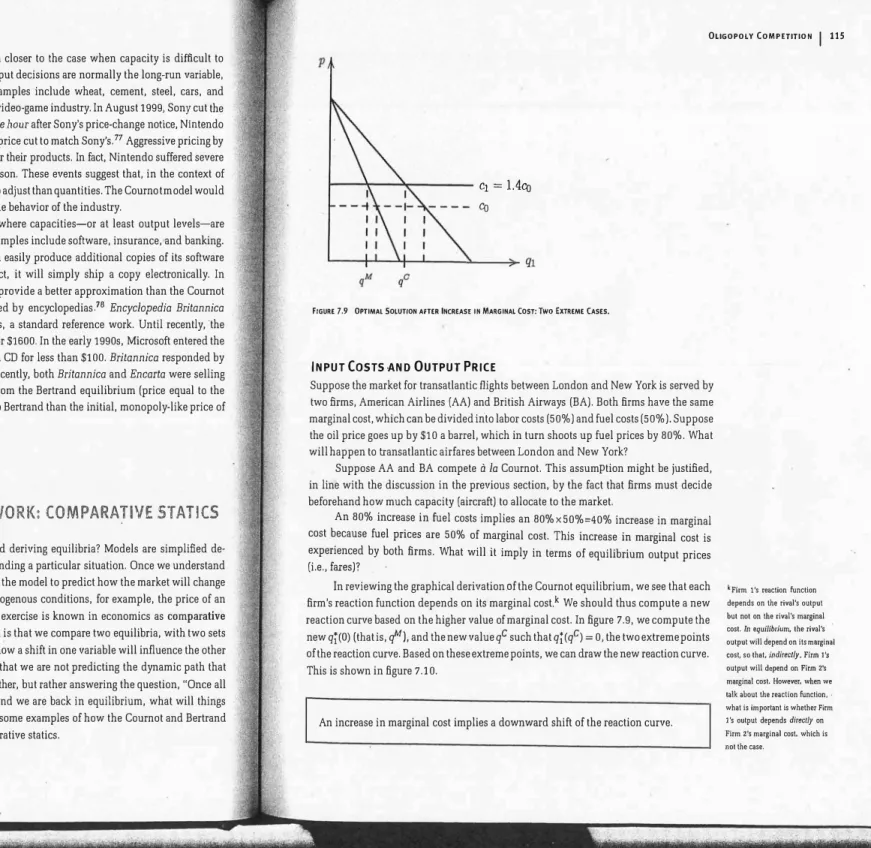
^{Cl =} 1.4O O

FIGURE 7.9 OPTIMAL SOLUTION AFTER INCREASE IN MARGINAL (OST: Two EXTREME CASES.

INPUT COSTS AND OUTPUT PRICE

Suppose the market for transatlantic flights between London and New York is served by two irms, American Airlines (AA) and British Airways (BA). Both irms have the same marginal cost, which can be divided into labor costs (50%) and fuel costs (50%). Suppose the oil price goes up by $10 a barrel, which in turn shoots up fuel prices by 80%. What will happen to ransatlantic airfares between London and New York?

Suppose AA and BA compete lla Coumot. This assumption might be justiied, in line with the discussion in the previous section, by the fact that irms must decide beforehand how much capacity (aircraft) to allocate to the market.

An 80% increase in fuel costs implies an 80% x50%=40% increase in marginal cost because fuel prices are 50% of marginal cost. This increase in marginal cost is experienced by both irms. What will it imply in terms of equilibrium output prices (i.e., fares)?

In reviewing the graphical derivation of the Coumot equilibrium, we see that each irm's reaction function depends on its marginal costk We should thus compute a new reaction curve based on the higher value of marginal cost. In igure 7.9, we compute the new _qr(O) (that is, _qM), and the new value _qC such that _qr(qc) = 0, the two extreme points of the reaction curve. Based on these extreme points, we can draw the new reaction curve. This is shown in igure 7.10.

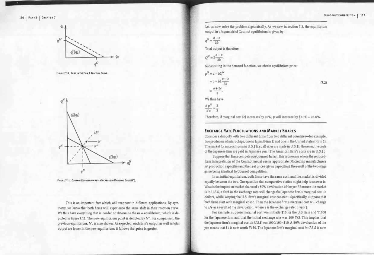
An increase in marginal cost implies a downward shift of the reaction curve.

k Firm 1 's reaction function depends on the rival's output but not on the rival's marginal cost. In equWbrium, the rival's output will depend on its marginal cost, so thet. indirect/y, Firm 1's output will depend on Firm 2's marginal cost. However, when we talk about the reaction funcHon, . what is important is whether Firm 1's output depends directly on Firm z's marginal cost. which is not the case.

116

I

^{PART 3}

I

^{CHAPTER 7}

FIGURE 7.10 SHIFT IN THE fiRM 1 REACTION (URVE.

fiGURE _7.11 (OURNOT EQUILIBRIUM AFTER 'NCREASE IN MARGINAL (OST _(N").

This is an important fact which will reappear in different applications. By sym­ metry, we know that both irms will experience the same shift in their reaction curve. We thus have everything that is needed to determine the new equilibrium, which is de­ picted in igure 7.11. The new equilibrium point is denoted by Nil. For comparison, the previous equilibrium, N', is also shown. As expected, each irm's output as well as total output are lower in the new equilibrium; it follows that price is greater.

OLIGOPOLY COMPETITION

_I

117

Let us now solve the problem algebraically. As we saw in section 7.3, the equilibrium output in a (symmetric) Coumot equilibrium is given by

Total output is therefore

Substituting in the demand function, we obtain equilibrium price: pN =0 ^_ bQN

= 0 _ b2° ^-_3b ^c 0 +2c

= -3-' We thus have

Therefore, if marginal cost (c) increases by 40%, P will increase by

_�

40% = 26.6%. EXCHANGE RATE FLUCTUATIONS AND MARKET SHARES

(7.2)

Consider a duopoly with two different irms rom two different countries-for example, two producers of microchips, one in Japan (Firm 1) and one in the United States (Firm 2). The market for microchips is in U.S.$ (Le., all sales are made in U.S.$). However, the costs of the Japanese irm are paid in Japanese yen. (The American irm's costs are in U.S.$.)

Suppose that irms compete a ¹⁰ Coumot. In fact, this is one case where the reduced· form interpretation of the Coumot model seems appropriate: Microchip manufacturers set production capacities and then set prices (given capacities), the result of the two-stage game being identical to Coumot competition.

In an initial equilibrium, both irms have the same cost, and the market is divided equally between the two. One question that comparative statics might help to answer is: What is the impact on market shares of a 50% devaluation of the yen? Because the market is in U.S.$, a shift in the exchange rate will change the Japanese irm's marginal cost in dolars, while keeping the U.S. irm's marginal cost constant. S^'peciica)ly, suppose that both irms start with marginal cost c. Then the Japanese irm's marginal' cost will change to cle as a result of the devaluation, where e is the exchange rate in yen/$.

For example, suppose marginal cost was initially $10 for the U.S. irm and Yl000 for the Japanese irm and that the initial exchange rate was 100 Y /$. This implies that the Japanese irm's marginal cost in U.S.$ was 1000/100=$10. A 50% devaluation of the yen means that $1 is now worth Y150. The Japanese irm's marginal cost

_in

U.S.$ is now

I ^I

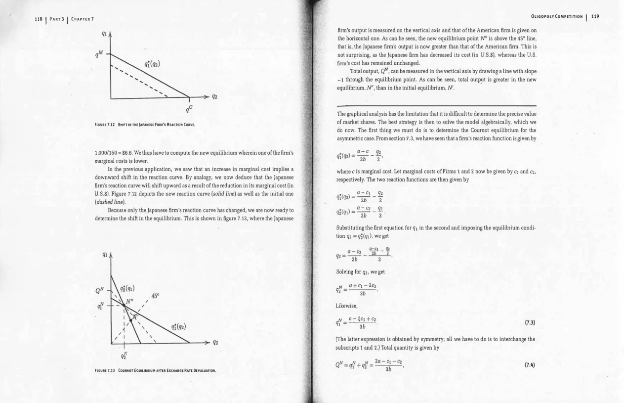
⁷

FIGURE 7.12 SHIfT IN THE JAPANESE FIRM'S REACTION CURVE.

1,000/150 = $6.6. We thus have to compute the new equilibrium wherein one of the irm's marginal costs is lower.

In the previous application, we saw that an increase in marginal cost implies a downward shift in the reaction curve. By analogy, we now deduce that the Japanese irm's reaction curve will shift upward as a result of the reduction in its marginal cost (in U.S.$). Figure 7.12 depicts the new reaction curve (solid line) as well as the initial one (dashed line).

Becaus

_�

only the Japanese irm's reaction curve has changed, we are now ready to determine the shift in the equilibrium. This is shown in igure 7.13, where the Japanese

q�

FIGURE 7.13 (OURNOT EQUILIBRIUM AFTER EXCHANGE RATE DEVALUATION.

irm's output is measured on the vertical axis and that of the American irm is given on the horizontal one. As can be seen, the new equilibrium point Nl is above the 45° line, that is, the Japanese irm's output is now greater than that of the American irm. This is not surprising, as the Japanese irm has decreased its cost (in U.S.$), whereas the U.S. irm's cost has remained unchanged.

Total output, QN, can be measured in the vertical axis by drawing a line with slope -1 through the equilibrium point. As can be seen, total outp�t is greater in the new equilibrium, Nl, than in the initial equilibrium, N'.

The graphical analysis has the limitation that it is diicult to determine the precise value oLmarket shares. The best strategy is then to solve the model algebraically, which we do now. The irst thing we must do is to determine the Coumot equilibrium for the asymmetric case. From section 7.3, we have seen that a irm's reaction function is given by

where

_C

is marginal cost. Let marginal costs afFirms 1 and

2

now be given by

_Cl

and cz, respectively. The two reaction functions are then given by

•

a-Cl qz

ql(qZ)

⁼

_{b -2}

• a

_{-Cz ql}

qZ(ql)

⁼

_b

-

_2'

Substituting the irst equation for

_ql

in the second and imposing the equilibrium condi­ tion

_qz

=

_qi(ql),

we get

Solving for

_qz,

we get N ^{a tel}

^-2cz

qz =

_3b

Likewise, N

a -�Cl

^t

Cz

ql

_{= 3b .}

^(7.3)

(The latter expression is obtained by symmetry; all we have to do is to interchange the subscripts 1 and

2.)

Total quantity is given by

(7.4)

120 I

^{PART 3}

I

^CHAPTER. 7

Finally, Firm l's market share., 51, is given by q1 0 - 2C1 + Cz

51=-=

q1 + qz 20 -C1 -Cz Calibration

(7.5)

Regarding the right-hand side of this equation, all we now is that, initially, C1 = Cz, whereas, after the devaluation, C1 = czle = czll.5. To derive the numerical value of 51,

we would have to obtain additional information regarding the initial equilibrium; based on that information, we must determine the values of 0 and c. The process of obtaining. values for the model parameters based on information about the equilibrium is known as calibration.

Suppose, for example, that before devaluation, output price was 13.33 and mar- ginal cost 10. From the previous application, we know that, in equilibrium,

0+2c p=-. ₃

where c is the initial value of marginal cost. Solving with respect to 0, we get 0= 3p -2c = 3(16.66) -2(10) = 20.

Because c = 10 is the initial value of marginal cost, after devaluation we have Cz = 10 and C1 ⁼ 10/1.5 = 6.66. Substituting these values in (7.5), we get

20 - 2 x 10/1.5 + 10 . I

51 = ₂ ." 71 �o.

x 20 -10/1.5 -10

In summary, a 50% devaluation of the yen increases the Japanese irm's market share to 71 % rom an initial 50%.

NEW TECHNOLOGY AND PROFITS

Consider the industry for some chemical product, a commodity that is supplied by two irms. Firm 1 uses an old technology and pays a marginal cost of $15. Firm 2 uses a modern technology and pays a marginal cost of $10. In the current equilibrium, price is at $16.66 and output at 8.33. How much would Firm 1 be willing to pay for the modern technology?

Quite simply, the amount that Firm 1 should be willing to pay for the technology is . the difference between its proits with lower marginal cost and its current proits. We thus have to determine Firm l's equilibrium proits in two possible equilibria and compute the difference. In a way, this problem is the reverse of the one examined before. In the case of exchange-rate devaluation, we started from a symmetric duopoly and moved to an asymmetric one. Now, we start rom n asymmetric duopoly (Firm 2 has lower marginal cost) and want to examine the shift to a symmetric duopoly, whereby Firm ₁ achieves the same marginal cost as its rival.

From (7.4), we know that total output is given by N N N 20 -C1 -^Cz

Q =q1 + qz = _3b

Substituting in the demand function, we get pN = 0 ^_ bQN = 0 + ^c

^�

+ Cz .

OLIGOPOLY COMPETITION

I 121

(7.6)

(Notice that, in the particular case when C1 = Cz = c, ^{we get} (7.2), the equilibrium price in the symmetric duopoly case.)

Given the expressions for Firm l's output (7.3) and for equilibrium price (7.6), we can now compute Firm l's equilibrium proits:

1f1 = pq1 -C1q1 0+C1+CZ

3 ^{q1 -c1q1}

(

^0+C1+CZ

₎

= ₃ -C q1

=

(

^0+C1+CZ -c

₎

^0+CZ-2Cl

3 3b

0+ Cz -2C1 0 + Cz -2C1

3 ^. 3b

=

^� ₍

^{0 + cZ}

3 ^-2C1

^r

Finally, the value that Firm 1 would be willing to pay for the improved technology would be the difference in the value of the preceding expression with C1 = 15 and C1 = 10. To determine the precise value, we need, once again, to calibrate the model.

By analogy with what was done in the previous application, we can invert the price equatio^'n (7.6) to obtain

0=3p-C1-CZ .

Because p = 16.66, C1 ⁼ 15, Cz = 10, this implies that 0 = 3 x 16.66 -15 -10 = 25. ^More­ over, (7.4) can be inverted to obtain

b= 20 -^{C1 -Cz} --3 -Q-=

Because Q = 8.33, it follows that b = (2 x 25 - 15 -10)/(3 ^x 8.33) = 1. T herefore, in the initial equilibrium, Firm l's proits are given by

f1 =

_C

5 + 10

; ^{2 x 15}

_r

⁼

_{G r '}

I

whereas, with the new technology, proits will be given by

rl =

C5 + 10;

^{2 x}

_lOr

=

_(¥r

We conclude that Firm 1 should be willing to pay

(15)2 (5)2 3 _- 3

^" 22.22 for the new technology.

Let us return to the issues from the beginning of this section. Why is it useful to perform comparative statics? Take, for example, the last application considered earlier. The question we posed was: How much would Firm

₁

(the ineicient irm) be willing to pay for an innovation that reduces marginal cost to

₁₀

(the eicient irm's cost level)? Our analysis produced an answer to this question: Firm

₁

would gain 22.22 rom adopting the more eicient technology.

Is it worth going through all the algebraic trouble to get this answer? A simpler estimaie for the gain might be the following: Take Firm l's initial output as given and compute the gain rom reducing marginal cost. Because initial output is

_1.66,

this

.^calcu­ lation would yield the number

1.66(15 - 10)

= 8,3. This number greatly underestImates the true gain. Why? The main reason is that, upon reducing marginal cost, Firm

₁

be­ comes much more competitive: Not only does it increase its margin, it also increases its output.

Let us then consider an alternative simple calculation. Because Firm

₁

will have a marginal cost identical to that of Firm 2, we can estimate the gain by the difference bet

_�

een Firm 2's and Firm l's initial proits. Firm 2's output (in the initial equilibrium) is

_6.66,

whereas price is given by

_16.66;

its proit is thus

6.66(16.66 - 10).

Firm 1, in turn, is starting rom a proit of

1.66(16.66 - 15).

We would thus estimate a gain of

6.66(16.66 - 10)

^minus

1.66(16.66 - 15),

which is approximately

_41.6.

This tinle we are grossly overestimating the true value. Why? The main reason is that, when Firm

1

becomes more aggressive (with a lower marginal cost), Firm

₂

reduces its output. In other words, the main reason why Firm 2 has such a high output (and proit) in the initial equilibrium is th

_�

t it faces an ineficient competitor. Moreover, when Firm

₁

reduces its marginal cost, the market becomes more competitive, that is, price goes down, whIch increases the estimate error rom using the initial equilibrium levels.

The advantage of the equilibrium analysis, that is, comparative statics, is that it , takes into account all of the effects that follow rom an exogenous change, such as a reduction in one irm's marginal cost. Taking the initial equilibrium values as constant may lead to gross misestimation of the impact of an exogenous change, especially if the change is Signiicant in magnitude (as in the example we have considered).

I

Naturally, this defense of comparative statics is based on the presumption that the equilibrium solution is sensible. This section concludes with an additional argument in favor of \he methodology we have been using.

A

" DYNAMI C" I NTERPRETATION OF TH·E (OURNOT EQUI LI BRI UM It is easy to understand why the Cournot equilibrium is a stable solution: No irm would have an incentive to choose a different output. In other words, each irm is choosing an optimal strategy given the strategy chosen by its rival. But, is the Cournot equilibrium a realistic prediction of what will happen in reality?

The equilibrium concept we have used is that of Nash equilibrium, irst introduced in chapter 4. There, we presented possible justiications for the concept of Nash equilib­ rium. Here, we present an argument, irst proposed by Cournot himself, which is similar to the idea of solution by elimination of dominated strategies.

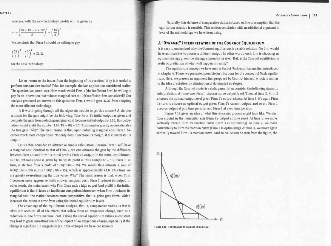
Although the Cournot model is a static game, let us consider the following dynamic interpretation. At time one, Firm 1 chooses some output level. Then, at time 2, Firm 2 chooses the optimal output level given Firm l's output choice. At time 3, it's again Firm l's turn to choose an optimal output given Firm 2's current output, and so on. Firm

₁

chooses output at odd time periods, and Firm 2 at even time periods.

Figure

_7.14

gives an idea of what this dynamic process might look like. We start rom a point in the horizontal axis (Firm 2's output at time zero). At time 1, we move vertically toward Firm l's reaction curve (Firm

₁

is optimizing). At time 2, we move horizontally to Firm 2's reaction curve (Firm 2 is optimizing). At time 3, we move again vertically toward Firm l's reaction curve. And so on. As can be seen from the igure, the

FIGURE 7.14 CONVERGENCE TO (OURNOT EQUILIBRIUM.

124

_I

^{PART 3}

_I

CHAPTE R 7

In fact, the point we are making here is more generally applicable to the justiication of Nash equilibria in a certain class of games. The argument we are using is similar to elimination of dominated strategies, a topic we dealt with in chapter 4.

m In fact, the dynamic process we consider earlier is not very realistic: At each moment in time, one of the irms is choosing n optimal output, assuming that the

dynamic process converges to the Coumat equilibrium. In fact,

no matter what the initial

situation, we always converge to the Nash equilibrium.

This is reassuring insofar as it provides an additional motivation for the idea of Cournot equilibrium l Moreover, it reinforces the idea that static models (like Cournot) are useful for comparative statics only. They do not describe the dynamic process that leads rom one equilibrium to another one. Static models give an idea of where the

"system" will converge after all of the interim adjustments have taken place.m

I

^SUMMARY

I

• Under price competition with homogeneous product and constant, symmetric mar­ ginal cost (Bertrand model), irms price at the level of marginal cost.

If irms set output or capacity levels (Cournot model). then duopoly output is greater than monopoly output and lower than perfect competition output. Likewise, duopoly price is lower than monopoly price and greater than price under perfect compe­ tition.

• If capacity and output can be easily adjusted, then the Bertrand model is a better ap­ proximation of duopoly competition. If;by contrast, output and capacity are diicult to adjust, then the Cournot model is a good approximation of duopoly competition.

K E Y CONCE PTS

• _oligopoly

• duopoly

• best response

• reaction function

• residual demand

rival's output remains constant, - comparative statics

which in fact does not occur except

in the Nash equilibrium. • calibration

OLIGOPOLY COMPETITION

_I

₁₂₅

[

R EV I E W AND PRACTI CE E X E RCISES

_I

7.1 According to Bertrand's theory, price competition drives irms' proits down to zero even if there are only two competitors in the market. Why don't we observe this in practice very often?

7.2 Three criticisms are frequently raised against the use of the Coumot oligopoly model: (1) irms normally choose prices, not quantities; (2) firms don't normally make their decisions simultaneously; (3) irms are requently ignorant of their rivals' costs; in fact, they do not use the notion of the Nash eqUilibrium when making their strategic decisions.

. How would you respond to these criticisms?

(Hint:

in addition to this chapter, you may want to refer to chapter

_4.)

7.3 Which model (Coumot, Bertrand) would you think provides a better approxi- mation to each of the following industries: oil reining, internet access, insurance. Why?

7.4* Two irms, CS Corporation and jl & Associates, make identical goods, GPX units, and sell them in the same market. The demand in the market is

_Q

= 1200 ^-

_p.

Once a irm has built capacity, it can produce up to its capacity each period with a marginal cost of Me ⁼ O. Building a unit of capacity costs 2400 (for either CS or jl) and a unit of capacity lasts four years. The interest rate is zero. Once production occurs each period, the price in the market adjusts to the level at which all production is sold. (In other words, these irms engage in quantity competition, not price competition.)

a. If CS knew that jl were going to build 100 units of capacity, how much would CS want to build? If CS knew that jl were going to build x units of capacity, how much would CS want to build (that is, what'is CS's best response function in capacity)? b. If CS and jl each had to decide how much capacity to build without knowing the

other's capacity decision, what would the one-shot Nash equilibrium be in the amount of capacity built?79

7.5" Consider a market for a homogeneous product with demand given by Q ⁼ 37.5 ^-

_p/4.

There are two irms, each with constant marginal cost equal to

_40.

a. Determine output and price under a Cournot equilibrium.

b. Compute the eficiency loss as a percentage of the eiciency loss under monopoly. 7.6" Show analytically that equilibrium price under Cournot is greater than price under perfect competition but lower than monopoly price.