FI ELD-PRO G RAM M ABLE G ATE ARRAY S
(FPGAs) are digital devices that implement logic circuits required by users in the field. Because of their short turnaround time, low manufacturing cost, and field programma- bility, interest in system prototyping and re- configuration using FPGAs has steadily increased. There are many different FPGA ar- chitectures, driven by different programming technologies. The type we consider here is SRAM-based, or lookup table, FPGAs, which users can reprogram any number of times. FPGA testing, like the testing of conven- tional digital integrated circuits, is indis- pensable to ensuring proper operation. Testing can be applied to either unpro- grammed or programmed FPGAs. Here, we focus on unprogrammed FPGAs, for which a number of researchers have proposed test- ing methodologies.1-4
FPGA fault diagnosis is also an important problem. Like testing, fault diagnosis also ap- plies to either unprogrammed or pro- grammed FPGAs. Fault diagnosis for unprogrammed FPGAs5is particularly im- portant. If engineers can identify and isolate a faulty part in an FPGA prior to program- ming it, they can implement a required log- ic function using only fault-free parts.
In this article, we introduce a universal fault diagnosis approach for unprogrammed FPGAs. Based on a test procedure for con-
figurable logic blocks (CLBs) developed by Michinishi et al.,4our procedure’s diagnostic resolution is one CLB; that is, it can locate a fault to just one CLB. The procedure’s com- plexity—the time required to perform a uni- versal fault diagnosis—for a sequentially loadable FPGA2is O(N2n log n), which de- pends on the FPGA’s array size. N is the FPGA’s array size, and n is the size of the lookup table.
If we can make universal diagnosis com- plexity independent of array size, we can re- duce complexity considerably. To that end, we propose a class of FPGAs with a univer- sal fault diagnosis procedure whose com- plexity is independent of array size. We call these C-diagnosable FPGAs. We will present another universal fault diagnosis procedure whose complexity is independent of array size N, and we will show its application to block-sliced, sequentially loadable FPGAs. FPGA architecture
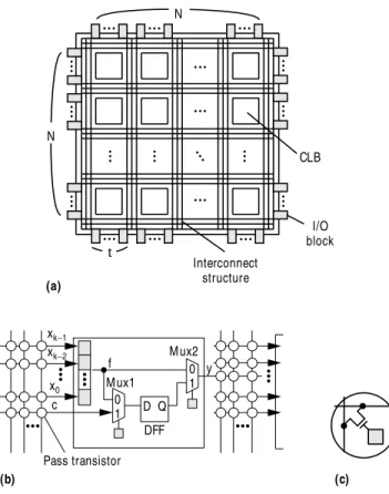
Figure 1 illustrates the FPGA architecture we consider in this article. The FPGA con- sists of an N× N array of programmable CLBs, programmable I/O blocks, and a pro- grammable interconnect structure. On each side of the FPGA are tN I/O blocks; in other words, the FPGA contains 4tN I/O blocks. Each CLB consists of one lookup table, two multiplexers, and one D flip-flop (DFF), con-
Universal Fault Diagnosis for
Lookup Table FPGAs
TO M O O IN O UE SATO SHI M IYAZAKI
HIDEO FUJIW ARA N ara Institute of Science and
Technology
Focusing on configurable logic blocks in a lookup table FPGA, the authors present universal fault
diagnosis procedures that can locate a fault to
just one CLB. The complexity of the proposed procedure for FPGAs using block-sliced
loading is independent of FPGA array size.
nected as shown in Figure 1b. A lookup table implements com- binational logic as a 2k×1 memory composed of configuration memory cells (CMCs), where k is the number of input lines of the lookup table. When one applies an input pattern to a lookup table, the table selects a CMC addressed by the input pattern, and the cell’s output provides the function’s value. A lookup table therefore can implement any of 2nfunctions of its inputs, where n equals 2k. In programming the FPGA, one loads the memory with the bit pattern corresponding to the func- tion’s truth table. In the CLB, the connections among the in- put and output lines, the lookup table, and the D flip-flop are configured as multiplexers controlled by CMCs.
An interconnect structure surrounds the CLBs, connecting them and the I/O blocks. A connection in the interconnect structure is configured as a pass transistor, also controlled by a CMC, as shown in Figures 1b and 1c.
One programs a lookup table FPGA by loading a program composed of a bit sequence into the FPGA’s CMCs. Storing each bit of the program in the corresponding CMC config- ures all the CLBs and interconnections, thus implementing a logic function in the FPGA. Such a logic function is called a configuration. The FPGA must contain circuitry that allows
program loading. The FPGA-programming scheme we con- sider here is sequential loading. This scheme shifts the pro- gram into the FPGA, storing each bit of the program in the corresponding CMC. An FPGA with this type of loading is called a sequentially loadable FPGA (SL-FPGA). When an SL-FPGA implements configurations, it loads all CMCs. Universal fault diagnosis
First, we introduce a procedure that locates a fault in any faulty programmed FPGA corresponding to an unpro- grammed FPGA. That is, it locates a fault in any faulty con- figuration implemented on the FPGA.
Fault model. Our approach applies to stuck-at, incorrect- access, nonaccess, and multiple-access faults of lookup ta- bles in CLBs, and functional faults of multiplexers and D flip-flops in CLBs.6We assume that several of these faults may occur in a CLB simultaneously and that the number of CLBs including these faults in an FPGA is at most one.
Universal test procedure. We denote the procedure4 for testing CLBs in SL-FPGAs as TPCLB. We perform this pro- cedure by repeatedly implementing a configuration and al- ternately applying an input sequence to the configuration. That is, we represent TPCLBby a sequence of pairs consisting of a configuration and an input sequence applied to the con- figuration as follows:
TPCLB= [(C1, S1), (C2, S2), …, (C2k+4, S2k+4)]
where Ciis the ith configuration, Siis the input sequence ap- plied to Ci, and k is the number of input lines of a lookup table. Tables 1 and 2 list the configurations and input se- quences in TPCLB. This test procedure can detect any fault defined in our fault model.
By applying TPCLBto each CLB in an FPGA implemented with a connection between the CLB and I/O blocks, we can identify faulty CLBs. However, this will consume much time. If we can configure connections so that we can apply the test procedure to all the CLBs simultaneously, we can locate the faulty ones immediately. However, the number of CLBs in an FPGA is N2= N×N, whereas the number of I/O blocks in an FPGA is O(N) = 4tN. Hence, if array size N becomes large, it will be impossible to configure such connections. Universal fault diagnosis procedure. Let’s assume in- put sequence Siat configuration Ciin TPCLB. Let Ribe the out- put sequence obtained by applying Sito a fault-free CLB that implements Ci. Earlier work4has shown that Rican be used as a certain bit sequence of Sifor other CLBs implementing the same configuration Ci. Therefore, if the output line of a CLB is connected with the appropriate input line of anoth-
N
N
xk−1 xk−2
x0
CLB
(a)
(b) (c)
Mux1
Mux2
DFF
c 0
1
0 1 f y
t
I/O block Interconnect
structure
Pass transistor D Q
Figure 1.FPGA architecture: N×N FPGA (a); CLB and interconnect structure (b); pass transistor (c). Shaded cubes in (b)and (c) are CMCs (mux: multiplexer).
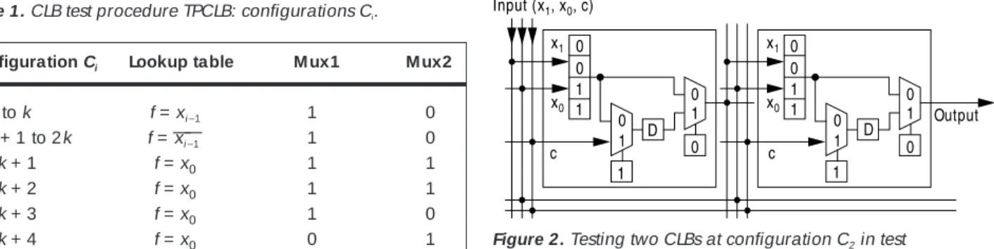
er CLB, we can simultaneously test multiple CLBs with a small number of I/O blocks. Figure 2 shows an example of such testing. Based on this idea, we previously presented a test procedure that connected several CLBs in a cascade to test all the CLBs in an FPGA concurrently.
However, our diagnostic resolution goal is one CLB. As long as we observe output responses from several CLBs via a single primary output implemented by an I/O block, as in Figure 2, we cannot see which CLB is faulty. Hence, to iden- tify just one faulty CLB by means of a limited number of I/O blocks, we must apply the test procedure several times as the configurations in the interconnect structure change. Now, let’s consider the number of test procedures required to locate a faulty CLB. Suppose that NOprimary outputs can be implemented at each configuration in the underlying test procedure. Then, the average number d of CLBs connected to a primary output—that is, the first test procedure’s diag- nostic resolution (the number of candidates for faulty CLBs)— is N2/NO. By applying the test procedure with different connections of CLBs again, we can further reduce the diag- nostic resolution to N2/NO2. We express the diagnostic reso- lution after applying the test procedure i times as di= N2/NOi. When NIprimary inputs are implemented to feed the same input sequences to all CLBs concurrently, the number NOof primary inputs that can be implemented is 4tN−NI. Since the number of input lines of a CLB is k + 1, NI= k + 1. Hence, NO= 4tN−(k + 1). Based on these equations, we can express the condition of the number i of test procedures needed for a diagnostic resolution of one CLB as N2≤[4tN−(k + 1)]i.
When i = 2, any FPGA satisfies this condition even if its ar- ray size N is large. Thus, we present a universal diagnosis procedure, DP1, that consists of two test steps. Each step tests all the CLBs concurrently in the same way as test procedure TPCLB. That is, we implement Cion each CLB and apply Sito all the CLBs for 1 ≤i≤2k + 4. As shown in Table 1, Ciand Si
are the configuration and input sequence in TPCLB. We can also express DP1as [(C1, S1), (C2, S2), …, (Cnc, Snc)], where
nc= 2(2k + 4) = 4k + 8 (1)
and ncis the number of configurations.
The difference between the two steps is the configuration of connections implemented on the interconnect structure (Figure 3, next page):
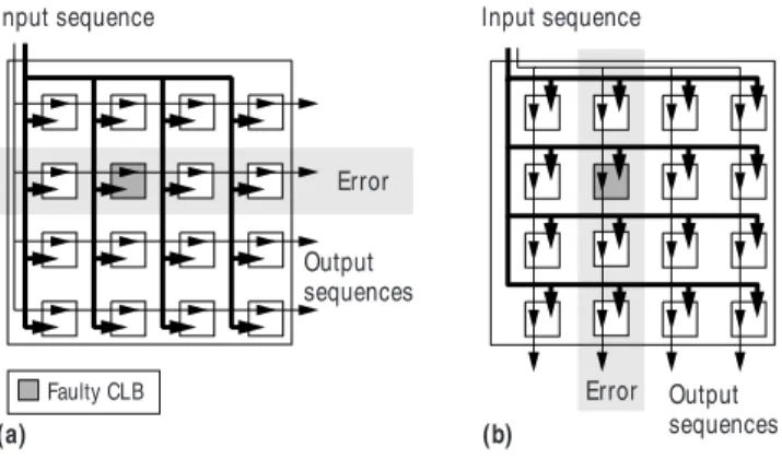
■ Step 1 (horizontal diagnosis). Let CLB(l, m) be the CLB at the lth column in the mth row. At all Ci, the output line of CLB(l, m) is connected with an appropriate input line of CLB(l + 1, m) for 1 ≤l≤N −1 for all m. The output line of the rightmost CLB(N, m) is connected with an I/O block as a primary output for all m. The other input lines are connected with remaining I/O blocks as primary outputs.
■ Step 2 (vertical diagnosis). Exchanging column num- ber l for row number m configures the interconnect structure the same way as in step 1.
Note that a cascade consisting of N CLBs is implemented on each row at step 1 (or on each column at step 2).
Table 1.CLB test procedure TPCLB: configurations Ci.
Configuration Ci Lookup table M ux1 M ux2
1 to k f = xi−1 1 0
k + 1 to 2k f = —xi−1— 1 0
2k + 1 f = x0 1 1
2k + 2 f = x0 1 1
2k + 3 f = x0 1 0
2k + 4 f = x0 0 1
Table 2.CLB test procedure TPCLB: input sequences Si.
Input sequence Si Input lines xk−1…x1 x0 Input line c
1 ≤i≤k 0…0 1, 0...1 0, …, 1…1 1, 0…0 0 (applied in this order) 0 (constant) k + 1 ≤i≤2k 0…0 1, 0…1 0, …, 1…1 1, 0…0 0 (applied in arbitrary order) 0 (constant)
2k + 1 0…0 0 (constant) 0, 0, 0, 1, 1, 0 (in this order)
2k + 2 ≤i≤2k + 4 0…0 0, 0…0 1, …, 1…1 1, 1…1 1 (applied in this order) 0, 1, 0, 1 (in this order) 0
0
c 0
1 D
0 1 0 1
0 0 1 1 1
1
c 0
1 D
0 1 0 1
Output x1
Input (x1, x0, c)
x0 x1
x0
Figure 2.Testing two CLBs at configuration C2in test procedure TPCLB.
In DP1, steps 1 and 2 identify the row and column re- spectively that include a faulty CLB with N primary outputs. As a result, DP1can identify just one CLB. This universal di- agnosis procedure is preset; that is, we execute step 2 irre- spective of step 1’s result.
Universal fault diagnosis complexity. We refer to the time required to perform a universal diagnosis procedure for an FPGA as the FPGA’s universal diagnosis complexity. As an example, let’s assume the following universal diag- nosis procedure for an FPGA G:
DP = [(C1, S1), (C2, S2), …, (Cnc, Snc)]
Let c(i) be the number of CMCs loaded to implement ith configuration Ci. Let s(i) be the length of input sequence Si
for Ci.
The time required to implement all the configurations in DP for G is
where tcis the time required to load one bit of a program into a CMC in G. The time required to apply all the input se- quences in DP for G is
where tsis the clock cycle time of a configuration imple- mented in G.
Thus, the universal diagnosis complexity of DP for G is (2)
Now, let’s consider DP’s universal diagnosis complexity for SL-FPGAs. When we change from one configuration to another on an SL-FPGA, we must load all the program bits. Hence, the time required to implement the configuration for DP for an SL-FPGA is c(i) = Nmfor all i, where Nmis the to- tal number of CMCs in G. As Equation 1 showed, the num- ber of configurations in DP is
nc= 2(2k + 4) = O(log n) (3)
where k is the number of input lines of a lookup table and n is the size of a lookup table. That is, n = 2k.
Without loss of generality, we assume the total number of CMCs in an FPGA is proportional to both the number of CLBs, N2, and the size of a lookup table (or the number of CMCs in a lookup table), 2k. That is, Nm= O(N2n), where n = 2k. Hence, the time required to implement all the configu- rations in DP1is
TSLC(DP1) = tcNmO(log n) = O(N2n log n) (4) Recall the configurations in test procedure TPCLB(Table 1). Note that each of the configurations C2k+1, C2k+2, and C2k+4
implements a path including a D flip-flop. Accordingly, each CLB cascade at the corresponding configurations in DP1in- cludes a shift register composed of N D flip-flops. Conse- quently, we can observe the output response for an input pattern N clock cycles later after applying the input pattern. From Table 1, the length s(i) of Siapplied to Ciin DP1is
Thus, the total time required to apply the input sequences in DP1is
TSLS(DP1) = [4kn + (2N + 10) + 8 + (4N + 12)]ts
= O(N + n log n) (5)
From Equations 4 and 5, the complexity of DP1for SL- FPGAs is
TSL(DP1) = O(N2n log n) (6)
This equation shows that the universal diagnosis complexi- ty of DP1for SL-FPGAs depends on the FPGA’s array size N. Making universal diagnosis complexity independent of array size would considerably reduce complexity. Next, we pre- sent another universal diagnosis procedure and a class of
s i
n i k k i k
N i k k
i k k
N i k k k k
( )
( , )
( , )
( , )
( , , , )
=
≤ ≤ + ≤ ≤ +
+ − = + +
= + +
+ − = + + + +
1 2 2 5 4 4
6 1 2 1 4 5
4 2 3 4 7
4 1 2 2 2 4 4 6 4 8
TG TGC TGS t c ic t s is
i nc
(DP)= (DP)+ (DP)= [ ( )+ ( )]
∑
= 1TGS t s ic
i nc
(DP)= ( )
∑
= 1TGC t c ic
i nc
(DP)= ( )
∑
= 1Input sequence Input sequence
Output sequences
Output sequences Error
Error Faulty CLB
(a) (b)
Figure 3.Universal diagnosis procedure DP1: step 1 (a) and step 2 (b).
FPGAs, called C-diagnosable FPGAs, for which universal di- agnosis complexity is independent of array size.
C-diagnosable FPGAs
Since an FPGA consists of an array of CLBs, we can con- sider it an iterative system. C-testable7is a term that describes an important class of testable iterative systems. An earlier work2extended the concept of C-testability for general LSI circuits to FPGAs. Here, we further extend the concept to FPGA fault diagnosis.
We define an FPGA as C-diagnosable if there exists a uni- versal fault diagnosis procedure whose complexity is inde- pendent of the FPGA’s array size. As we saw in Equation 6, the universal diagnosis complexity of DP1depends on the array size, and hence with DP1an FPGA is not C-diagnos- able. As shown by Equation 2, a universal diagnosis proce- dure’s complexity is the sum of the total configuration implementation time and the total input sequence applica- tion time. From Equations 4 and 5, we see that both imple- mentation time and application time of DP1for SL-FPGAs depend on array size. Here, we describe methods for mak- ing both times independent of array size.
First, let’s consider the application time of input se- quences in DP1. As mentioned earlier, there are configura- tions that implement shift registers in DP1, and the application time for such configurations depends on array size. A CLB lookup table can implement any k-input logic function. Therefore, we connect the output lines of multi- ple CLBs to the input lines of another CLB that implements an exclusive-OR (XOR). Then we can observe the multiple CLBs’ output responses from the XOR’s output without cas- cades of D flip-flops.
Thus, by modifying part of the configurations in DP1, we obtain another universal diagnosis procedure, DPC. Figure 4 illustrates the modification. We substitute the following two configurations for configuration Ciin DP1for i = 2k + 1, 2k + 2, 2k + 4, 4k + 5, 4k + 6, 4k + 8.
1) Ci′for all rows m (respectively all columns l ):
■ For h = 1, 2, …, N/2, the CLB at the odd column (row), CLB(2h −1, m) (CLB(l, 2h −1)), as well as its input lines, implements the same configuration as Ciin DP1.
■ For h = 1, 2, …, N/2, the CLB at the even column (row), CLB(2h, m) (CLB(l, 2h)), implements a 2-input XOR.
■ For h = 1, 2, …, N/2 −1, the output line of CLB(2h, m) (CLB(l, 2h)) connects to an input line of the XOR on CLB(2h + 2, m) (CLB(l, 2h + 2)).
■ The output line of the rightmost (bottommost) CLB, CLB(N, m) (CLB(l, N)), connects to an I/O block. 2) Ci′′: By exchanging the even CLBs for the odd ones, we
implement these configurations the same way as we implement Ci′.
DPCpartitions CLBs into two groups: N/2 CLBs that are di- agnosed and N/2 CLBs that configure N/2-input XORs to compress the output sequences from diagnosed FPGAs. DPC
exchanges these groups’ roles by means of the doubled con- figurations. As a result, configurations in DPCinclude no cas- cades of D flip-flops; accordingly, we can observe the output responses just one cycle later after applying the corre- sponding input pattern.
Consequently, although the number of configurations in- creases, the application time becomes independent of ar- ray size N. After substituting 2(6 ×2) and 2(4 ×4) for (2N + 10) and (4N + 12) in Equation 5, the total time required to ap- ply the input sequences in DPCis
TSLS(DPC) = (4kn + 24 + 8 + 32)ts= O(n log n) (7) which is independent of N.
Next, let’s consider the configuration time of this univer- sal fault diagnosis procedure. At the 12 substituted configu- rations just described, we implement a configuration to be diagnosed and an XOR alternately in each row or in each column. Hence, if we regard 2 ×2 CLBs—CLB(l, m), CLB(l, m + 1), CLB(l + 1, m), CLB(l + 1, m + 1) for l, m = 1, 3, 5, …— as one block, we implement an iterative system at any of the substituted configurations. Also, each CLB implements the same logic function at any other configuration in DPC. There- fore, we can see that DPCalways implements iterative sys- tems in which each logic block consists of 2 ×2 CLBs. To this diagnosis procedure, we can adapt the programming scheme called block-sliced loading.2An FPGA with block- sliced loading can load the same program into each block concurrently.
Let tbbe the time required to load the same program bit into the corresponding CMC in each block. The number of CMCs in a block is Nb= 22O(n) = O(n) , where n is the size of a lookup table. On the other hand, as mentioned earlier, when we derive DPCfrom DP1, we double six configurations in DP1. Hence, from Equation 3, the number of configura- tions in DPCis nc= 2(2k + 4) + 6 = O(log n). Therefore, the
Figure 4.Modification of DP1to DPC.
D D
D D
D D D D
2h−1 2h 2h+1 2h+2 C
in DPi1
C´ in DPc
i
C´´ in DPc
i
time required to implement configurations in DPCon a block-sliced SL-FPGA is
TBSSLC (DPC) = tbNbO(log n) = O(n log n) (8) Note that the application time of input sequences does not depend on the programming scheme. Therefore, from Equations 7 and 8, the universal fault diagnosis complexity of DPCfor block-sliced SL-FPGAs is TBSSL(DPC) = O(n log n). Thus, we can obtain C-diagnosable FPGAs.
WE HAV E I N TRO D UCEDtwo important concepts: universal and C-diagnosable. Since our proposed fault diagnosis pro- cedure is universal—independent of the logic functions to be realized—we need not provide a different diagnosis pro- cedure for each logic function. Further, our proposed FPGA is C-diagnosable—the time required to diagnose the FPGA is independent of its array size. This means that diagnosis complexity does not increase even if FPGA array size be- comes large. Therefore, our approach can be applied to large and complex FPGA systems. Although this article considered only faults in CLBs, diagnosis should also address faults in other components (interconnect structure, I/O blocks). In future work, we plan to investigate diagnosis procedures for all FPGA faults.
Acknow ledgments
We thank Takuji Okamoto, Tokumi Yokohira, and Hiroyuki Mi- chinishi of Okayama University, Japan, and Toshimitsu Masuzawa and Michiko Inoue of Nara Institute of Science and Technology for their helpful comments and discussions.
References
1. W.K. Huang and F. Lombardi, “An Approach for Testing Pro- grammable/Configurable Field Programmable Gate Arrays,” Proc. 14th IEEE VLSI Test Symp., IEEE Computer Society Press, Los Alamitos, Calif., 1996, pp. 450-455.
2. T. Inoue et al., “Universal Test Complexity of Field-Program- mable Gate Arrays,” Proc. Fourth IEEE Asian Test Symp., IEEE CS Press, 1995, pp. 259-265.
3. M. Renovell, J. Figueras, and Y. Zorian, “Test of RAM-Based FP- GAs: Methodology and Application to the Interconnect,” Proc. 15th IEEE VLSI Test Symp., IEEE CS Press, 1997, pp. 230-237. 4. H. Michinishi et al., “A Test Methodology for Configurable Log- ic Blocks of Lookup Table Based FPGAs,” IEICE Trans. D-I, Vol. J79-D-I, No. 12, Dec. 1996, pp. 1141-1150 (in Japanese). 5. X.T. Chen, W.K. Huang, and F. Lombardi, “On the Diagnosis of
Programmable Interconnect Systems: Theory and Applica- tion,” Proc. 14th IEEE VLSI Test Symp., IEEE CS Press, 1996, pp. 204-209.
6. T. Inoue, S. Miyazaki, and H. Fujiwara, “On the Complexity of
Universal Fault Diagnosis for Lookup Table FPGAs,” Tech. Re- port NAIST-IS-TR97020, Graduate School of Information Sci- ence, Nara Institute of Science and Technology, 1997 (http://isw3.aist-nara.ac.jp/IS/TechReport2/report/97020.ps). 7. A.D. Friendman, “Easily Testable Iterative Systems,” IEEE Trans.
Computers, Vol. C-22, No. 12, Dec. 1973, pp. 1061-1064.
Tomoo Inoue is an instructor at the Gradu- ate School of Information Science, Nara In- stitute of Science and Technology, Japan. His research interests include test generation, syn- thesis for testability, and parallel processing. Inoue received the BE, ME, and PhD from Meiji University, Kawasaki, Japan. He is a member of the IEEE, the Institute of Electronics, Information, and Communication Engineers of Japan, and the Information Pro- cessing Society of Japan.
Satoshi Miyazaki is with the Tenri Integrated Circuits Group, Sharp Corporation, Nara, Japan, where he is engaged in microprocessor devel- opment. He received the BE from Okayama University and the ME from the Nara Institute of Science and Technology, where he partici- pated in the work described in this article.
Hideo Fujiwara is a professor at the Graduate School of Information Science, Nara Institute of Science and Technology, Japan. His research interests are logic design, digital systems de- sign and test, VLSI CAD, and fault-tolerant com- puting. Previously, he held positions at Osaka University and Meiji University. He is the au- thor of Logic Testing and Design for Testability (MIT Press, 1985). Fu- jiwara received the BE, ME, and PhD from Osaka University. He is a fellow of the IEEE, a member of the Institute of Electronics, Infor- mation, and Communication Engineers of Japan, and a member of the Information Processing Society of Japan.
Send questions and comments about this article to Tomoo Inoue, Graduate School of Information Science, Nara Institute of Science and Technology, Ikoma, Nara 630-01, Japan; inoue@ is.aist-nara.ac.jp.