Power Constrained Preemptive TAM Scheduling
Erik Larsson and Hideo Fujiwara
Graduate School of Information Science
Nara Institute of Science and Technology,
8916-5 Takayama, Ikoma, Nara 630-0101, Japan
Abstract1We integrate scan-chain partitioning and preemptive test access mechanism (TAM) scheduling for core-based systems under power constraint. We also outline a flexible power conscious test wrapper to increase the flexibility in the scheduling process by (1) allowing several different bandwidths at cores and (2) controlling the cores test power consumption, which makes it possible to increase the test clock. We model the scheduling problem as a Bin-packing problem and we discuss the transformations: (1) TAM-time and (2) power-time and the possibilities to achieve an optimal solution and the limitations. We have implemented our proposed preemptive TAM scheduling algorithm and through experiments we demonstrate its efficiency.
1 Introduction
To manage the increasing complexity of digital systems, the core-based design technique, SOC (system-on-chip), has been developed. The approach shows similarities with PCB (printed circuit board) design technique, however, from a testing perspective, there are differences; one is the amount of test data. In both approaches test data is transported in and out of the system but for PCB systems the amount is less since components are tested prior to mounting, which is not the case for cores in core-based designs. In addition, due to the design complexity, a substantial amount of test data is transported in and out of an SOC design leading to long testing times.
Scheduling techniques minimizing the test time have been proposed [3,20,4,18,8,1,12,13,14]. Recently TAM scheduling, a special case of test scheduling, has gained interest [7,9]. An important issue then is the wrapper used to connect the cores to the TAM [11,15,16,17]. Techniques have also been proposed to reduce test power dissipation allowing testing at higher clock frequencies [6,19,21].
In this paper, we combine preemption-based test scheduling [8] and scan-chain partitioning [1] to a preemptive TAM scheduling technique under power constraint, which we modelled as a Bin-packing problem. We also outline a flexible power conscious test wrapper, which is useful to (1) control the test power at cores, (2) control the test power at system level and (3) allow flexibility bandwidth at each core. We discuss the possibility to achieve an optimal solution using the transformations given due to preemption and flexible bandwidth. We also have analysed previously proposed test architecutures for different TAM bandwidths. For the
flexible wrapper, our algorithm determines the cores that require a flexible wrapper and the number of flexible configurations.
The paper is organized as follows. An overview of related work is in Section 2, and preliminaries are given in Section 3. The system model and the problem formulation are given in Section 4. In Section 5, we analyse previous proposed techniques and our approach is described in Section 6. Experimental results are presented in Section 7 and the paper is concluded in Section 8.
2 Related Work
Scheduling the tests in a system means that start time and end time are determined for all tests while satisfying all constraints minimizing the test time. Several techniques have been proposed and they can be divided into:
• Non partitioned testing with techniques proposed by Zorian [20] and Chou et al.[4], see Figure 1(a),
• Partitioned testing with run to completion with work done by Chakrabarty [3] and Muresan et al. [18], see Figure 1(b) for illustration, and
• Partitioned (preemptive) testing where Iyengar and Chakrabarty [8] proposed a technique, see Figure 1(c). All approaches minimize test time but are taking different issues in consideration. Chakrabarty focus on test conflicts imposed by external and BIST (Built-In Self-Test) tests [3]. Zorian’s technique minimizes the number of control lines for BIST systems under power constraint [20]. For general systems, Chou et al. [4] and Muresan et al. [18] have proposed techniques considering power and conflicts.
The above test scheduling approaches focus on a fixed test time for all test sets. Iyengar and Chakrabary proposed
1. This work has been supported by the Japan Society of Promo-
tion of Science (JSPS) under grant P01735. Figure 1. Scheduling approaches.
t2a
(c) Partitioned testing t5
t1 t4
t3 t2b (b) Partitioned testing with run to completion
t2
t5 t4
t1 t3
(a) Nonpartitioned testing
session 1 session 2 session 3
t2 t5
t4 t1
t3
7th IEEE European Test Workshop, pp. 411- 416, May 2002.
a preemption-based test scheduling technique [8] where each test set can be interrupted and resumed later.
In scan testing each test vector is shifted in (scanned in), and after a capture cycle, the test response is shifted out (scanned out). This process contributes to a major part of the test time. It can be reduced by partitioning the scan flip flops into several chains of shorter length. Aerts and Marinssen [1] investigated scan-chain partitioning where the constraints are defined by available pins (bandwidth).
The shift process also contributes to a major part of the test power consumption [6]. Gerstendörfer and Wunderlich [6] proposed a technique to isolate the scan flip-flops during the shift process. However, the approach may cause an effect on the critical path.
Test access is eased by placing the core in a wrapper such as Boundary scan [2], TestShell [15], or IEEE P1500 [16]. These approaches assume one single TAM bandwidth per core. However, using a wrapper library a flexible bandwidth design is possible [17]. Koranne has recently proposed a flexible bandwidth test wrapper [11].
3 Preliminaries
Cores in a core-based design environment are given as [2]:
• soft cores, which comes in the form of synthesizable RTL (register-transfer level) descriptions,
• firm cores, supplied as gate-level netlists, or as
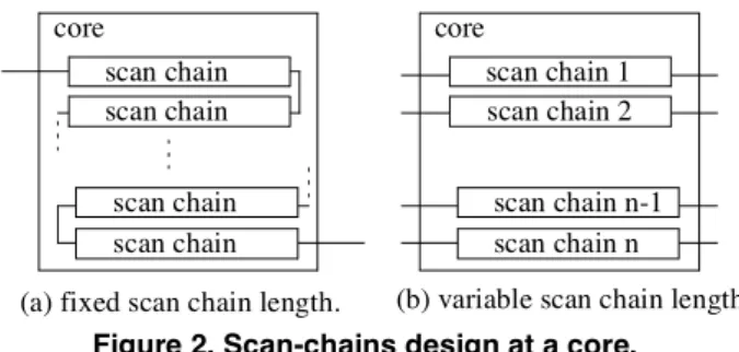
• hard cores, available as non modifiable layouts. The soft cores allow more flexibility compared to firm cores and hard cores. This is also true when determining the type of test method. For scan-based testing, soft cores allow a higher flexibility when determining the number of scan- chains and their length. However, when creating a hard core flexibility to determine the number of scan-chains and their length can be achieved. Consider an example of a hard core and its scan chain implementation in Figure 2. In Figure 2(a) a single scan chain is used while in (b) a fixed set of n scan chains is used. In both cases the number of scan chains are fixed, however, in Figure 2(b) the chains can externally be configured into a variation of scan chain lengths. Furthermore, in order to design a hard core, which is easier to reuse, many short scan-chains of equal length is to be preferred compared to few scan-chains of unequal length.
The advantage of the approach in Figure 2(b) is not only that a variety of scan chain lengths can be achieved but also that the test power dissipation can be decreased [21]. In Figure 2(b), when a single scan-chain is assumed, it is possible to activate only one partition of the scan-chain at any time. By dividing the scan chain into several of shorter length, the activity in the scan chain is reduced and since the test power highly depends on the activity the consumed power is only 1/n in Figure 2(b) compared to (a).
In Figure 3 we demonstrate how to achieve a flexible scan chain length for a hard core. Depending on the selectors the two partitions can form either a single scan chain or two scan chains. The decode logic (Figure 3) is used to switch off the unused scan-chain in order to reduce the activity in the not used sub-scan chain. If a single scan- chain is assumed, the test vectors are loaded through tam1 and using the selectors it is possible to direct the test vector to the right sub-chain. When both chains are loaded at the same time, test data is loaded in scan chain 1 through tam1 and in scan chain 2 through tam2. In this case clock1 and clock2 are active at the same time. The multiplexer on the output is used to direct the test response to right TAM wire.
The advantage of our approach is that we can achieve a flexible TAM bandwidth at each core and also that we can control the test power dissipation at each individual core.
4 System Modelling and Problem Formulation
An example of a system under test is given in Figure 4 where each core is placed in a wrapper in order to ease test access. The system is tested by applying several sets of tests to the system where each set is created at a test generator (source) and the test response is analysed at a test response evaluator (sink). A system under test, such as the one shown in Figure 4, can be modelled as:
C= {c1, c2,..., cn} is a finite set of n cores. Each core ci∈C is characterized by: tpi: test power when active, tvi: number of test vectors, ffi: number of scanned flip-flops. For the system:
Ntam: bandwidth of the test access mechanism, and Pmax: maximal allowed power at any time.
The test time and the test power consumption for a set of test vectors activating niscan chains are defined below. The test Figure 2. Scan-chains design at a core.
scan chain core
scan chain
scan chain scan chain
scan chain 1 core
scan chain 2
scan chain n scan chain n-1
(a) fixed scan chain length. (b) variable scan chain length
Figure 3. Flexible power conscious scan-chains design at a core test wrapper.
core
scan chain 2 wrapper
scan chain 1
clock tam1
tam2
decode clock2 clock1
tam1
mux mux tam2
select1
select2
Figure 4. Embedded cores, wrappers and TAM. core c1
wrapper scan-chain 1 scan-chain 2
test source test sink
test access mechanism (tam)
scan-chain n
core cn wrapper
scan-chain 1 scan-chain 2
scan-chain n
time for a scan tested core ciis given by [1]:
at a core with ffiscanned flip-flops partitioned into niscan chains and tvitest vectors.
Based on the discussion above the test power at a core ci depends on the activity in the system, which depends on the number of active scan chains:
For each core, a set of test vectors is given and for a given TAM bandwidth, we can compute its test time and its power consumption using Eq. 1 and 2, which can be illustrated using a 3-dimensional cube for each test set as in Figure 5. Each test set has such a cube and all cubes has to be packed, scheduled minimizing time and full filling constraints, which is a Bin-packing problem [5].
In preemptive scheduling, the test vectors at each core do not have to be scheduled as a single test set. Each test set can be divided into several sub test sets. An example illustrating preemption based scheduling is in Figure 1(c) where test 2 is split into two partitions, 2a and 2b. Furthermore, the TAM bandwidth for each sub test set can be different. For instance, if we have a test set of 10 test vectors and we apply 5 in the first sub set and the other 5 in a second sub set, we can have one TAM bandwidth for the first set and another bandwidth for the second test set. To support this (preemption), we introduce; for a core ciwith test vectors to be applied in session j:
scij: number of test vectors, ttij: test time,
tamij: number of TAM wires required,
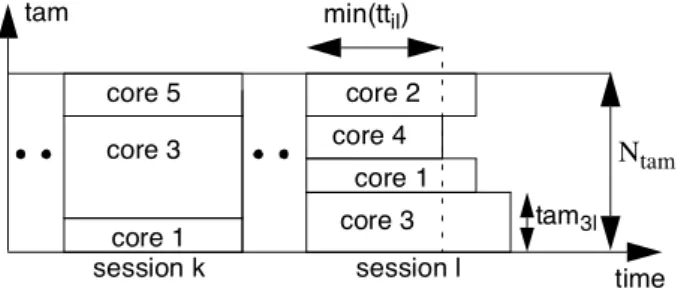
tpij(=tpi*tamij): test power consumed when active. An example is in Figure 6, where 3 scan chain partitions sc1kfrom core c1, sc3kfrom core c3and sc5kfrom core c5 are scheduled in session k.
For each test session we have to:
• select from which cores to include test vectors,
• select the number of test vectors in each partition,
• determine the number of scan-chains for each partition,
• determine the number of TAM wires for each partition,
• determine an end time for each of the partitions. with the objective to minimize the total test time while considering test power consumption.
We have introduced a set of transformations that we can apply to each test set in order to determine its test time, TAM usage and power dissipation and we also have introduced preemptive testing used to sub divide each test set. Combining the transformations and preemption means that we have a high degree of flexibility in the test scheduling process both when it comes to determine the test
time and the test power consumption at each core. It also means that we have to check for the possibility of achieving an optimal solution by either assign all TAM wires to each core in a sequence or by dividing each test set into several very small test sets, which easily can be scheduled. However, there are a number of factors limiting both of these approaches:
1. scan-chains are not allowed to be too short,
2. the assignment of TAM wires for a core may not al- ways result in an integer result:
3. dividing the test set into several test sets increases the total test time, and
4. a high TAM size results in a higher “area” per test. For point 3, assume we have a core with a test set of 10 vectors, 20 flip-flops and a single TAM wire. Its test time is given by: (10+1)×20/1+10=230. If the test set is divided into two sets, each with 5 test vectors the test time is: (5+1)×20/1+5+(5+1)×20/1+5=250.
For point 4, compute the product (“area”) given by test time×TAM wires for the test set above assuming a single TAM wire and 10 TAM wires. In the case with one single TAM wire the product is: ((10+1)×20/1+10)×1=230 and in the case with 10 TAM wires the product is: ((10+1)×20/ 10+10)×10=320.
5 Analysis of Previous Test Architectures
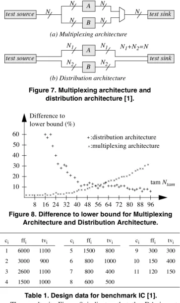
In this section, we analyze the MA (Multiplexing architecture) and the DA (Distribution architecture) (Figure 7) [1]. In MA each core is given all TAM bandwidth when it is to be tested, which means the tests are scheduled in a sequence. For cores where the number of scan-chains is smaller than the TAM bandwidth, the TAM is not fully utilized. Furthermore, since the test time is minimized at each core, the test power is maximized, which could damage the core.
In DA, each core is given its dedicated part of the TAM, which means that initially all cores occupy a part of the TAM. The approach assumes that the bandwidth of the TAM is at least as large as the number of cores, (Ntam>|C|).
We have made an analysis of the test time on the IC benchmark (Table 1) for the MA and the DA where scan chains must include at least 20 flip flops and where the size of the TAM is in the range |C|<Ntam<96, Figure 8. The lower bound of the test time, excluding the capture cycles and the shift out of the last response, is given by [1]:. tt es t( )ci = (tvi+1)× ffi⁄ni +tvi 1
pt es t( )ci = tpi×ni 2
Figure 5. A three dimensional view of the problem. test time
test power testacc
essmec hanism
pmax Ntam
tpi tami
tvi
Figure 6. Session length based on preemption.
session k session l
tam
time core 5
core 3
core 1
core 1 core 3
core 2 core 4 min(ttil)
tam3l Ntam
∆i = ffi⁄ni +ffi⁄ni 3
ffi×tvi Ntam ---
i=1 C
4
The results in Figure 8 indicates that the DA is not efficient for low TAM size while MA is less efficient as the TAM size increases,
6
The Preemptive TAM Scheduling Algorithm In this section, we describe the PTS (preemptive TAM scheduling) algorithm, which is outlined in Figure 9. The objective is to minimize the total test time while satisfying all constraints and the power limitation. The idea is to assign TAM wires to the cores in each session such that Equation 3 is minimized. The algorithm starts by trying to find sessions with a single core fully utilizing the TAM. The number of cores in a session is increased until |C|. If not all vectors are scheduled, the allowed fault (∆) increases and the algorithm restarts. The algorithm terminates when all test vectors are scheduled.In Figure 6 core 1,2,3 and 4 have been chosen to be included in session l. The tam assignment for each core has been completed and the session length (preemption time) is determined by min(ttil), see Figure 6.
Figure 6 also illustrates that each core can be assigned to a different number of TAM wires when its test vectors are split up into several sessions, i.e tam3kis not equal to tam3l.
7 Experimental Results
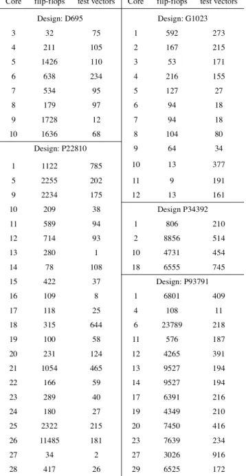
We have made a comparison between the MA (multiplexing architecture) [1], the DA (distributed architecture) [1] and our proposed PTS (preemptive TAM scheduling) technique (Figure 9). The three approaches have been implemented and the benchmarks we have used are the IC benchmark [1] and the ITC’02 benchmarks, D695, G1023, P22810, P34392 and P93791 [10]. The data for the IC benchmark is in Table 1. For the ITC’02 benchmarks, we excluded the U220 since it only contains one scan tested core. We excluded all non-scan tested cores and assumed that scan- chains can be freely determined. The ITC’02 benchmarks as we used them are presented in Table 2.
For every benchmark we made experiments at 12 different TAM bandwidths. In the cases where there is no result for the DA, it is due to the technique cannot be used when the TAM size is less than the number of cores.
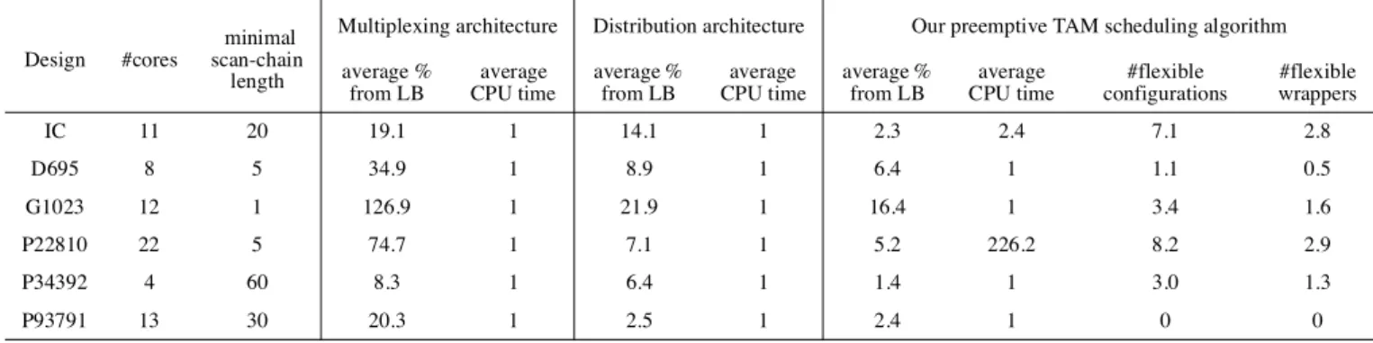
All experiments were performed on a SunBlade 1000, 900 MHz with 1024 Mb RAM memory and all experimental results are collected in Table 5 and the results are summarized in Table 4.
The experimental results in Table 5 are organized as follows. For each benchmark, we have made experiments at 12 different TAM bandwidths. We have for each of the scheduling techniques collected the test time, the difference to lower bound and the computational cost (CPU time). The test time is given as the time when the last test finish and the lower bound is computed using Eq. 4. For our approach, we have also computed the number of cores with flexible wrappers and the number of flexible configurations, which are used to indicate the introduced overhead. The overhead is counted as follows. For all cores requiring one TAM bandwidth, there is no cost. However, as soon as more than one configuration is required, we count all needed configurations including the first. For instance, at design IC at TAM bandwidth 8, 7 wrapper configurations are needed,
ci ffi tvi ci ffi tvi ci ffi tvi
1 6000 1100 5 1500 800 9 300 300
2 3000 900 6 800 1000 10 150 400
3 2600 1100 7 800 400 11 120 150
4 1500 1000 8 600 500
Table 1. Design data for benchmark IC [1]. Figure 7. Multiplexing architecture and
distribution architecture [1].
test sink N
test sink A
A B
B N
N N
N test source N
test source
N1+N2=N N1
N1
N2 N2
(a) Multiplexing architecture
(b) Distribution architecture
Figure 8. Difference to lower bound for Multiplexing Architecture and Distribution Architecture.
tam Ntam Difference to
lower bound (%) 60
40
20 10 30 50
8 16 24 32 40 48 56 64 72 80 88 96 :distribution architecture :multiplexing architecture
j=0/session number /
∆=initial value; Rtam=ΣNi
until |C| = 0 begin / all test vectors at all cores scheduled / for k= 1 to |C| begin
for all possible SCjwhere |SCj|=k and tamij≤Niand Σ tamij=min(Ntam,R) and Σ ∆i≤∆ and Σ tpij≤Pmax begin
t=min(ttij) / length of session / for all scij∈SCjbegin
scij=(t×tamij-ffi)/(tamij+ffi) / vectors in session j / tvi=tvi-scij / preempt test vectors /
if tvi=0 then begin R=R-Ni
remove cifrom C end
end
j=j+1 / new session / end
end
∆=∆+δ / increase allowed fault / end
Figure 9. Preemptive TAM scheduling algorithm.
which are distributed over 3 wrappers where 2 wrappers have 2 configurations each and 1 wrapper has 3 configurations (2+2+3). For each benchmark we have also computed the average test time, average CPU time and for our approach the average number of wrapper configurations and the average number of flexible wrappers.
For every bandwidth at all benchmarks our approach produces a solution with the test time closest to lower bound. The computational cost using the MA and the DA are extremely low. We have a slightly higher computational cost, but in most of the cases we only require a few seconds. Our approach assumes flexible wrappers, which has a cost but both the number of flexible wrappers and the number of wrapper configurations are low.
For the IC benchmark (first group in Table 5) we let the
TAM width be in the range from 8 to 96 in steps of 8 and we did not allow any scan chain include less than 20 scan flip flops. Our approach finds the solution with the test time closest to the lower bound for all bandwidths. The computational cost for the MA and the DA approaches are below 1 second, however, our approach requires only 2.4 seconds on average.
A TAM schedule on the IC benchmark at TAM size 40 is presented in Table 3. The schedule consists of 11 sessions and for each session, its test time is shown as well as the cores tested, their TAM assignment and the number of test vectors. The total test time is equal to the summation of the test time at each test session.
The TAM schedule (Table 3) demonstrates also how our algorithm proceeds. Our algorithm starts by trying to assign all TAM wires to one core. After trying all cores, the algorithm tries combinations with two cores and continues to increase the number of cores on until |C| is reached. If not all test vectors are scheduled, the algorithm restarts, with one core and continuous until all test vectors are scheduled. A re-start, is performed after session 8 (there are two cores scheduled at session 9 and one in session 10).
The TAM schedule (Table 3) also demonstrates the use of flexible wrappers. For cores that appear only once in the schedule, only one TAM bandwidth is assigned to those cores and a flexible wrapper is not needed. An example of such a core is core 11 (Table 3). An example of a core that appears several times is core 5, which appears in 5 different sessions. However, core 5 does not require 5 different TAM bandwidths, only 4 since it uses 30 TAM wires in both session 6 and 8. For this TAM schedule (Table 3), we need 2 flexible wrappers; one for core 5 and one for core 8. The flexible wrapper at core 5 requires 4 configurations and the flexible wrapper at core 8 requires 2 configurations; in total 6 configurations.
For D695, G1023, P22810, P34392 and P93791 the results in Table 5 shows that our approach finds a solution closest to the lower bound. In all cases, the computational cost is low. Only at P22810 the computational cost is higher, however, it is still in the range of a few minutes. Furthermore, the additional overhead due to the flexible wrapper is low. Only a few cores require a flexible wrapper with only a few configurations at each such core wrapper.
Core flip-flops test vectors Core flip-flops test vectors
Design: D695 Design: G1023
3 32 75 1 592 273
4 211 105 2 167 215
5 1426 110 3 53 171
6 638 234 4 216 155
7 534 95 5 127 27
8 179 97 6 94 18
9 1728 12 7 94 18
10 1636 68 8 104 80
Design: P22810 9 64 34
1 1122 785 10 13 377
5 2255 202 11 9 191
9 2234 175 12 13 161
10 209 38 Design P34392
11 589 94 1 806 210
12 714 93 2 8856 514
13 280 1 10 4731 454
14 78 108 18 6555 745
15 422 37 Design: P93791
16 109 8 1 6801 409
17 118 25 4 108 11
18 315 644 6 23789 218
19 100 58 11 576 187
20 231 124 12 4265 391
21 1054 465 13 9527 194
22 166 59 14 9527 194
23 289 40 17 6391 216
24 180 27 19 4349 210
25 2322 215 20 7450 416
26 11485 181 23 7639 234
27 34 2 27 3026 916
28 417 26 29 6525 172
Table 2. Design data for the ITC’02 benchmarks D695, G1023, P22810, P34392 and P93791.
S Time Core - c, TAM wires - t, Vectors - v 0 8420 c:7 t:40 v:400
1 21020 c:6 t:40 v:1000 2 72665 c: 3 t:40 v:1100 3 68475 c: 2 t:40 v:900 4 166250 c: 1 t:40 v:1100
5 9330 c: 8 t:30 v:443 c: 9 t:10 v:300 6 3537 c: 5 t:30 v:68 c: 8 t:10 v:57 7 51050 c: 4 t:30 v:1000 c: 5 t:10 v:337
8 4680 c: 5 t:30 v:90 c:10 t: 6 v:179 c:11 t: 4 v:150 9 5771 c: 5 t:34 v:124 c:10 t:6 v:221
10 7097 c: 5 t:40 v:181 Σ 418295
Table 3. TAM schedule for benchmark IC at TAM size 40.
8 Conclusions
In this paper, we have combined preemptive TAM scheduling and scan-chain partitioning for scan tested core- based systems under power constraint.
We have also outlined a core test wrapper allowing a flexible scan chain length at cores and allowing a control of the power consumption at each core. The advantage with a possibility of a flexible bandwidth is that it increases the flexibility in the scheduling process and the advantage of having a mechanism to control the test power consumption at core-level is that it makes it possible to increase the test clock frequency.
We have made an analysis of previously proposed techniques and modelled the problem as a Bin-packing problem. Experiments comparing our implementation with other approaches show that our technique produces solutions with the lowest test time at a low computational cost and a low overhead due to more complex wrappers.
References
[1] J. Aerts and E. J. Marinissen, “Scan Chain Design for Test Time Reduction in Core-Based ICs”, Proceedings of IEEE International Test Conference (ITC), pp. 448-457, Washington, DC, October 1998.
[2] M. L. Bushnell and V. D. Agrawal, “Essentials of Electronic Testing for Digital, Memory, and Mixed-Signal VLSI Circuits”, Kluwer Academic Publ., ISBN 0-7923-7991-8. [3] K. Chakrabarty, “Test Scheduling for Core-Based Systems
Using Mixed-Integer Linear Programming”, IEEE Transactions on CAD of IC and Systems., Vol. 19, No. 10, pp. 1163-1174, Oct. 2000.
[4] R. Chou et al., “Scheduling Tests for VLSI Systems Under Power Constraints”, IEEE Transactions on VLSI Systems, Vol. 5, No. 2, pp. 175-185,June 1997.
[5] T. Cormen, C. Leiserson, and R. Rivest, “Introduction To Algorithms”, The MIT Press, ISBN 0-262-03141-8, 1989. [6] S. Gerstendörfer and H-J Wunderlich, “Minimized Power
Consumption for Scan-Based BIST”, Proceedings of IEEE International Test Conference (ITC), pp. 77-84, Atlantic City, NJ, Sep. 1999.
[7] Y. Huang et al., “Resource Allocation and Test Scheduling for Concurrent Test of Core-Based SOC Design”, Proceedings of IEEE Asian Test Symposium (ATS), pp. 265- 270, Kyoto, Japan, Nov. 2001.
[8] V. Iyengar and K. Chakrabarty, “Precedence-based, preemptive, and power-constrained test scheduling for system-on-a-chip”, Proceedings of IEEE VLSI Test Symposium (VTS), pp. 42-47, CA, April 2001.
[9] V. Iyengar et al., “Test Wrapper and Test Access Mechanism Co-Optimization for System-on-Chip”, Proceedings of IEEE International Test Conference (ITC), pp. 1023-1032, Baltimore, MD, Nov. 2001.
[10] ITC´02 (International Test Conference) SOC Benchmarks, http://www.extra.research.philips.com/itc02socbenchm/. [11] S. Koranne, “Design of Reconfigurable Access Wrappers for
Embedded Core Based SOC Test”, Proceedings of IEEE International Symposium on Quality Electronic Design (ISQED), pp 106-111, San Jose, California, March 2002. [12] E. Larsson and Z. Peng, “An Integrated System-On-Chip
Test Framework”, Proceedings of Design, Automation and Test in Europe Conference (DATE), pp. 138-144, Munchen, Germany, March 2001.
[13] E. Larsson and Z. Peng, “The Design and Optimization of SOC Test Solutions”, Proceedings of IEEE/ACM International Conference on Computer-Aided Design (ICCAD), pp. 523-530, San Jose, CA, Nov. 2001.
[14] E. Larsson and Z. Peng, “Test Scheduling and Scan-Chain Division Under Power Constraint”, Proc. of IEEE Asian Test Symposium (ATS), pp. 259-264, Kyoto, Japan, Nov. 2001. [15] E. J. Marinissen et al., “A Structured and Scalable
Mechanism for Test Access to Embedded Reusable Cores”, Proceedings of IEEE International Test Conference (ITC), pp. 284-293, Washington, DC, Oct. 1998.
[16] E. J. Marinissen et al., “Towards a Standard for Embedded Core Test: An Example”, Proc. of IEEE International Test Conference (ITC), pp. 616-627, Atlantic City, NJ, Sep. 1999. [17] E. J. Marinissen et al., “Wrapper Design for Embedded Core Test”, Proceedings of IEEE International Test Conference (ITC),pp. 911-920, Atlantic City, NJ, Oct. 2000.
[18] V. Muresan et al., “A Comparison of Classical Scheduling Approaches in Power-Constrained Block-Test Scheduling”, Proceedings of IEEE International Test Conference (ITC), pp. 882-891, Atlantic City, NJ, Oct. 2000.
[19] N. Nicolici and B. M. Al-Hashimi, “Power Conscious Test Synthesis and Scheduling for BIST RTL Data Paths”, Proceedings of IEEE International Test Conference (ITC), pp. 662-671, Atlantic City, NJ, Oct. 2000.
[20] Y. Zorian, “A distributed BIST control scheme for complex VLSI devices”, Proceedings of IEEE VLSI Test Symposium (VTS), pp. 4-9, Atlantic City, NJ, April 1993.
[21] J. Saxena et al., “An Analysis of Power Reduction Techniques in Scan Testing”, Proceedings of IEEE International Test Conference (ITC), pp. 670-677, Baltimore, MD, Oct. 2001.
Design #cores
minimal scan-chain
length
Multiplexing architecture Distribution architecture Our preemptive TAM scheduling algorithm average %
from LB
average CPU time
average % from LB
average CPU time
average % from LB
average CPU time
#flexible configurations
#flexible wrappers
IC 11 20 19.1 1 14.1 1 2.3 2.4 7.1 2.8
D695 8 5 34.9 1 8.9 1 6.4 1 1.1 0.5
G1023 12 1 126.9 1 21.9 1 16.4 1 3.4 1.6
P22810 22 5 74.7 1 7.1 1 5.2 226.2 8.2 2.9
P34392 4 60 8.3 1 6.4 1 1.4 1 3.0 1.3
P93791 13 30 20.3 1 2.5 1 2.4 1 0 0
Table 4. Summery of the experimental results.
Design
TAMwidth
Distribution Architecture Multiplexing Architecture Our PTS, Preemptive TAM Scheduling Lower bound
Testtime Differenceto lowerbound(%) CPU(s) Testtime Differenceto lowerbound(%) CPU(s) Testtime Differenceto lowerbound(%) CPU(s) #flexiblewrapper configurations #flexible wrappers Testtime
IC
8 Not applicable 2068931 0.6 <1 2065770 0.5 1 7 3 2056000
16 1652600 60.8 <1 1045764 1.7 <1 1036738 0.8 <1 6 2 1028000
24 945758 38.0 <1 707115 3.2 <1 693288 1.2 <1 5 2 685333
32 661700 28.7 <1 537240 4.5 <1 521038 1.4 <1 5 2 514000
40 478934 16.5 <1 436338 6.1 <1 418295 1.7 2 6 2 411200
48 389753 13.7 <1 376179 9.8 <1 349524 2.0 3 9 4 342666
56 321200 9.4 <1 331535 12.9 <1 299025 1.8 <1 8 3 293714
64 288461 12.2 <1 297802 15.9 <1 263468 2.5 1 5 2 257000
72 251250 10.0 <1 272477 19.3 <1 240453 5.3 6 11 4 228444
80 221300 7.6 <1 252758 22.9 <1 211582 2.9 <1 6 2 205600
88 201200 7.6 <1 240146 28.5 <1 194506 4.1 3 7 3 186909
96 181100 5.7 <1 228635 33.4 <1 176344 2.9 8 11 4 171333
Average: 19.1 1 14.1 1 2.3 2.4 7.1 2.8
D695
4 Not applicable 135360 2.0 <1 135360 2.0 <1 0 0 132696
8 158396 138.7 <1 68422 3.1 <1 68422 3.1 <1 0 0 66348
12 75199 70.0 <1 46174 4.4 <1 46174 4.4 <1 0 0 44232
16 50289 51.6 <1 35077 5.7 <1 34806 4.9 <1 4 2 33174
20 31856 20.0 <1 28193 6.2 <1 27898 5.1 <1 6 3 26539
24 25727 16.3 <1 23900 8.1 <1 23347 5.6 1 5 2 22116
28 22476 18.6 <1 20649 8.9 <1 20411 7.7 <1 7 3 18956
32 19034 14.8 <1 18199 9.7 <1 17759 7.1 <1 8 4 16587
36 17183 16.5 <1 16384 11.1 <1 15933 8.1 <1 2 1 14744
40 15274 15.1 <1 14977 12.9 <1 14371 8.3 <1 0 0 13269
44 13319 10.4 <1 14054 16.5 <1 13218 9.6 1 7 3 12063
48 12320 11.4 <1 13131 18.7 <1 12250 10.8 <1 2 1 11058
Average: 34.9 1 8.9 1 6.4 1 3.4 1.6
G1023
10 Not applicable 29448 10.7 <1 28361 6.6 <1 3 1 26608
12 162481 632.8 <1 24935 12.5 <1 24904 12.3 6 2 1 22173
14 54525 186.9 <1 21379 12.5 <1 21041 10.7 <1 2 1 19006
16 36287 118.2 <1 18997 14.2 <1 18483 11.1 1 0 0 16630
18 32879 122.4 <1 17120 15.8 <1 16400 10.9 <1 0 0 14782
20 23563 77.1 <1 15860 19.2 <1 15324 15.2 1 0 0 13304
22 18359 51.8 <1 14522 20.1 <1 13735 13.6 43 0 0 12094
24 17003 53.4 <1 13564 22.4 <1 12965 16.9 55 0 0 11086
26 15069 47.2 <1 12907 26.1 <1 12212 19.3 1 0 0 10234
28 12877 35.5 <1 12089 27.2 <1 11491 20.9 2 2 1 9503
30 12055 35.9 <1 11541 30.1 <1 10722 20.9 123 2 1 8869
32 11233 35.1 <1 11010 32.4 <1 10073 21.1 2 2 1 8315
Average: 126.9 1 21.9 1 16.4 24.8 1.1 0.5
Table 5. Experimental results of IC [1], D695, G1023, P22810, P34392, and P93791 [10] using multiplexing architecture [1], distribution architecture [1], and our preemptive TAM scheduling (PTS) technique.
P22810
8 Not applicable 661774 1.3 <1 661774 1.3 75 0 0 653454
16 Not applicable 333432 2.1 <1 333418 2.0 136 0 0 326727
24 882677 305.2 <1 223983 2.8 <1 223037 2.4 150 21 7 217818
32 393359 140.8 <1 169653 3.9 <1 168550 3.2 150 15 6 163363
40 229186 75.4 <1 137365 5.1 <1 136753 4.6 237 6 2 130690
48 167399 53.7 <1 115305 5.9 <1 114014 4.7 150 7 2 108909
56 130857 40.1 <1 100268 7.4 <1 98413 5.4 150 5 2 93350
64 110291 35.0 <1 88372 8.2 <1 86621 6.0 150 7 2 81681
72 95367 31.3 <1 79676 9.7 <1 77274 6.4 252 8 4 72606
80 80957 23.9 <1 73362 12.3 <1 70808 8.4 352 5 2 65345
88 71927 21.1 <1 66788 12.4 <1 63742 7.3 353 7 2 59404
96 65771 20.8 <1 62250 14.3 <1 59359 9.0 145 18 6 54454
Average: 74.7 1 7.1 1 5.1 226.2 8.2 2.9
P34392
8 2153059 46.6 <1 1474419 0.4 <1 1474419 0.4 <1 0 0 1469074
16 816123 11.1 <1 740855 0.9 <1 739207 0.6 1 2 1 734537
24 538719 10.0 <1 499534 2.0 <1 493126 0.7 <1 3 1 489691
32 380584 3.6 <1 377930 2.9 <1 370504 0.9 <1 3 1 367268
40 306605 4.4 <1 305824 4.1 <1 297019 1.1 <1 2 1 293814
48 253894 3.7 <1 257527 5.2 <1 247498 1.1 <1 5 2 244845
56 216124 3.0 <1 223593 6.5 <1 213427 1.7 <1 4 2 209867
64 189483 3.2 <1 197098 7.3 <1 187342 2.0 <1 4 2 183634
72 169434 3.8 <1 177012 8.4 <1 165515 1.4 <1 3 1 163230
80 152954 4.1 <1 161097 9.7 <1 149510 1.8 <1 2 1 146907
88 137263 2.8 <1 150725 12.9 <1 135687 1.6 3 4 2 133552
96 126819 3.6 <1 142129 16.1 <1 125887 2.8 1 4 2 122422
Average: 8.3 1 6.4 1 1.3 1.1 3.0 1.3
P93791
8 Not applicable 3081717 0.6 <1 3081717 0.6 <1 0 0 3064398
16 2775758 81.2 <1 1544043 0.8 <1 1544043 0.8 <1 0 0 1532199
24 1394819 36.6 <1 1032830 1.1 <1 1032446 1.1 <1 0 0 1021466
32 929174 21.3 <1 776871 1.4 <1 776487 1.4 <1 0 0 766099
40 744599 21.5 <1 624244 1.9 <1 623860 1.8 <1 0 0 612879
48 598779 17.2 <1 522517 2.3 <1 522133 2.2 <1 0 0 510733
56 473915 8.3 <1 450159 2.8 <1 449775 2.7 <1 0 0 437771
64 444521 16.0 <1 394439 3.0 <1 394055 2.9 1 0 0 383049
72 372518 9.4 <1 352728 3.6 <1 352344 3.5 <1 0 0 340488
80 345692 12.8 <1 318273 3.9 <1 317889 3.7 <1 0 0 306439
88 306818 10.1 <1 290426 4.3 <1 290042 4.1 1 0 0 278581
96 278767 9.2 <1 266769 4.5 <1 266385 4.3 1 0 0 255366
Average: 20.3 1 2.5 1 2.4 1 0 0
Design
TAMwidth
Distribution Architecture Multiplexing Architecture Our PTS, Preemptive TAM Scheduling Lower bound
Testtime Differenceto lowerbound(%) CPU(s) Testtime Differenceto lowerbound(%) CPU(s) Testtime Differenceto lowerbound(%) CPU(s) #flexiblewrapper configurations #flexible wrappers Testtime
Table 5. Experimental results of IC [1], D695, G1023, P22810, P34392, and P93791 [10] using multiplexing architecture [1], distribution architecture [1], and our preemptive TAM scheduling (PTS) technique.
![Table 5. Experimental results of IC [1], D695, G1023, P22810, P34392, and P93791 [10] using multiplexing architecture [1], distribution architecture [1], and our preemptive TAM scheduling (PTS) technique.](https://thumb-ap.123doks.com/thumbv2/123deta/5753246.27111/7.892.114.784.140.1088/experimental-multiplexing-architecture-distribution-architecture-preemptive-scheduling-technique.webp)
![Table 5. Experimental results of IC [1], D695, G1023, P22810, P34392, and P93791 [10] using multiplexing architecture [1], distribution architecture [1], and our preemptive TAM scheduling (PTS) technique.](https://thumb-ap.123doks.com/thumbv2/123deta/5753246.27111/8.892.111.783.132.1096/experimental-multiplexing-architecture-distribution-architecture-preemptive-scheduling-technique.webp)
