Mining by Itemset Maintenance
Chia-Hui Chang and Shi-Hsan Yang
Department of Computer Science and Information Engineering, National Central University, Chung-Li, Taiwan 320
chia@csie.ncu.edu.tw, carry@db.csie.ncu.edu.tw
Abstract. Incremental association mining refers to the maintenance and utilization of the knowledge discovered in the previous mining op- erations for later association mining. Sliding window filtering (SWF) is a technique proposed to filter false candidate 2-itemsets by segmenting a transaction database into several partitions. In this paper, we extend SWF by incorporating previously discovered information and propose two algorithms to boost the performance for incremental mining. The first algorithm FI SWF (SWF with Frequent Itemset) reuses the fre- quent itemsets of previous mining task as FUP2 to reduce the number of new candidate itemsets that have to be checked. The second algorithm CI SWF (SWF with Candidate Itemset) reuses the candidate itemsets from the previous mining task. Experiments show that the new proposed algorithms are significantly faster than SWF.
1 Introduction
Association rule mining from transaction database is an important task in data mining. The problem, first proposed by [2], is to discover associations between items from a (static) set of transactions. Many interesting works have been published to address this problem [9, 8, 11, 1, 6, 7, 10]. However, in real life applications, the transaction databases are changed with time. For example, Web log records, stock market data, and grocery sales data, etc. In these dynamic databases, the knowledge previously acquired can facilitate successive discovery processes, or become obsolete due to behavior change. How to maintain and reuse such knowledge is called incremental mining.
Incremental mining was first introduced in [4] where the problem is to up- date the association rules in a database when new transactions are added to the database. The proposed algorithm, FUP, stores the counts of all the frequent itemsets found in a previous mining operation and iteratively discover (k + 1)- itemsets as the Apriori algorithm [2]. An extension to the work is addressed in [5] where the authors propose the FUP2 algorithm for updating the exist- ing association rules when transactions can be deleted from the database. In essence, FUP2 is equivalent to FUP for the case of insertion, and is, however, a complementary algorithm of FUP for the case of deletion.
In the recent years, several algorithms, including the MAAP algorithm [13] and the PELICAN algorithm [12], are proposed to solve the problem incremental
mining. Both MAAP and PELICAN are similar to FUP2 algorithm, but they only focus on how to maintain maximum frequent itemsets when the database are updated. In other words, they do not care non-maximum frequent itemsets, therefore, the counts of non-maximum frequent itemsets can not be calculated. The difference of these two algorithms is that MAAP calculates maximum fre- quent itemsets by Apriori-based framework while PELICAN calculates maxi- mum frequents itemsets based on vertical database format and lattice decompo- sition.
As we know, Apriori-like algorithms tend to suffer from two inherent prob- lems, namely (1) the occurrence of a potentially huge set of candidate itemsets, and (2) the need of multiple scans of databases. To remedy these problems, Lee et al. proposed a sliding window filtering technique for incremental association mining [3]. By partitioning a transaction database into several partitions, SWF employs the minimum support threshold in each partition to filter unnecessary candidate itemsets such that the information in the prior partition is selectively carried over toward the generation of candidate itemsets in the subsequent par- titions. It is shown that SWF maintains a set of candidate itemsets that is very close to the set of frequent itemsets and outperforms FUP2 in a great deal. However, SWF does not utilize previously discovered frequent itemsets which are used to improve incremental mining in FUP2. In this paper, we show two simple extensions of SWF which significantly improve the performance by in- corporate previously discovered information such as the frequent itemsets or candidate 2-itemsets from the old transaction database.
The rest of this paper is organized as follows. Preliminaries on association mining are illustrated in Section 2. The idea of extending SWF with previously discovered information is introduced in Section 3. Experiments are presented in Section 4. Finally, the paper concludes with Section 5.
2 PRELIMINARIES
Let I={i1, i2, ..., im} be a set of literals, called items. Let D be a set of trans- actions, where each transaction T is a set of items such that T ⊆ I. Note that the quantities of items bought in a transaction are not considered, meaning that each item is a binary variable representing if an item was bought. Each trans- action is associated with an identifier, called T ID. Let X be a set of items. A transaction T is said to contain X if and only if X ⊆ T . An association rule is an implication of the form X → Y , where X ⊂ I, Y ⊂ I and X ∩ Y =Ø. The rule X → Y holds in the transaction set D with confidence c if c% of the transac- tions in D that contain X also contain Y . The rule X → Y has support s in the transaction set D if s% of transactions in D contain X ∪ Y . For a given pair of confidence and support thresholds, the problem of association rule mining is to find out all the association rules that have confidence and support greater than the corresponding thresholds. This problem can be reduced to the problem of finding all frequent itemsets for the same support threshold [2].
For a dynamic database, old transactions (△−) are deleted from the database
D and new transactions (△+) are added. Naturally, △− ⊆ D. Denote the up- dated database by D′, therefore D′ = (D − △−) ∪ △+. We also denote the set of unchanged transactions by D−= D − △−.
2.1 The SWF algorithm
In [3], Lee, et al., proposed a new algorithm, called SWF algorithm for incre- mental mining. The key idea of SWF algorithm is to compute a set of candidate 2-itemsets as close to L2 as possible. The concept of algorithm is described as follows. Suppose the database is divided into n partitions P1, P2, . . . , Pn, and processed one by one. For each frequent itemset I, there must exist some parti- tion Pk such that I is frequent from partition Pk to Pn. If we know a candidate 2-itemset is not frequent from the first partition where it presents frequent to current partition Pk, we can delete this itemset even though we don’t know if it is frequent from Pk+1 to Pn. If somehow this itemset is indeed frequent, it must be frequent in some partition Pk′, where we can add it to the candidate set again.
The SWF algorithm maintains a list of 2-itemsets CF that is frequent for the lasted partitions as described below. For each partition Pi, SWF adds frequent 2-itemsets (together with its starting partition Pi and supports) that is not in CF and checks if the present 2-itemsets are continually frequent from its’ start partition to the current partitions. If a 2-itemset is no longer frequent, SWF deletes this itemset from CF . If an itemset becomes frequent at partition Pj
(j > i), the algorithm put this itemset into CF and check it’s frequency from Pj to each successive partition Pj′ (j′ > j). It was shown that the number of the reserved candidate 2-itemsets will be close to the number of the frequent 2-itemsets.
For a moderate number of candidate 2-itemsets, scan reduction technique [9] can be applied to generate all candidate k-itemsetsss. Therefore, one database scan is enough to calculate all candidate itemsets’ supports and determine the frequent ones. In summary, the total number of database scans is kept as small as 2.
However, SWF does not utilize previously discovered frequent itemsets as applied in FUP2. In fact, for most frequent itemsets, the supports can be updated by simply scan the changed partitions of the database. It doesn’t need to scan the whole database for these old frequent itemsets. Only those newly generated candidate itemsets have to be checked by scanning the total database. In such cases, we can speed up not only candidate generation but also database scanning. The algorithm will be described in the next section.
2.2 An Example
In the following, we use an example to introduce how to improve the SWF algo- rithm. The example is the same as [3]. Figure 1(a) shows the original transaction database where it contains 9 transactions, tagged t1,. . .,t9, and the database is segmented into three partition, P1,P2,P3 (denoted by db1,3). After the database
(a) The 1st mining (b) The 2nd mining
Fig. 1. Example
is updated (delete P1and add P4), the database contains partition P2,P3,P4(de- noted by db2,4) as shown in Figure 1(b). The minimum support is assumed to be s= 40%. The incremental mining problem is decomposed into two procedures:
1. Preprocessing procedure which deals with mining in the original trans- action database.
2. Incremental procedure which deals with the update of the frequent item- sets for an ongoing time-variant transaction database.
Preprocessing procedure In the preprocessing procedure, each partition is scanned sequentially for the generation of candidate 2-itemsets. Consider this example in Figure 1(a). After scanning the first segment of 3 transactions, can- didate 2-itemsets {AB, AC, AE, AF, BC, BE, CE} are generated, and frequent itemsets {AB, AC, BC} are added to CF2 with two attributes start partition P1 and count. Note that SWF begins from 2-itemset instead of 1-itemset.
Similarly, after scanning partition P2, the occurrence counts of candidate 2-itemsets in the present partition are recorded. For itemsets that are already in CF2, add the occurrence counts to the corresponding itemsets in CF2. For itemsets that are not in CF2, record the counts and its start partition from P2. Then, check if the itemsets are frequent from its start partition to current partition and delete those non-frequent itemsets from CF2. In this example. The counts of the three itemsets {AB, AC, BC} in P2, which start from partition P1, are added to their corresponding counts in CF2. The local support (or called the filtering threshold) of these 2-itemsets is given by ⌈(3 + 3) ∗ 0.4⌉ = 3. The other candidate 2-itemsets of P2, {AD, BD, BE, CD, CF, DE}, has filtering threshold
⌈3 ∗ 0.4⌉ = 2. Only itemsets with counts greater than its filtering threshold are kept in CF2, others are deleted. Finally, partition P3 is processed by algorithm SWF. The resulting CF2={AB, AC, BC, BD, BE}.
After all partitions are processed, the scan reduction technique is employed to generate C3′ from CF2. Iteratively, Ck+1′ can be generated from Ck′ for k =
3, . . . , n, as long as all candidate itemsets can been stored in memory. Finally, we can find ∪kLk from ∪kCk with only one database scan.
Incremental procedure Consider Figure 1(b), when the database is updated form db1,3 to db2,4 where transaction, t1 t2 t3, are deleted from the database and t10, t11, t12 are added to the database. The incremental step can be divided into three sub-steps: (1) generating C2 in D− = db1,3- △− (2) generating C2
in db2,4 = D−+△+ (3) scanning the database db2,4 for the generation of all frequent itemsets Lk. In the first sub-step, we load CF2and check if the counts of itemsets in CF2will be influenced by deleting P1. We decrease the influenced itemstes’ counts that are suppored by P1and set the start position of influenced itemsets to 2. Then, we check the itemsets of CF2 from the start position of the itemsets to partition P3, and delete non frequent itemsets of CF2. It can be seen that itemsets {AB, AC, BC} were removed. Now we have CF2 corresponding to db2,3.
The second sub-step is similar to the operation in the preprocessing step. We add the counts of the 2-itemset in P4 to the counts of the same itemsets of CF2, and reserve the frequent itemsets of CF2. New frequent 2-itemsets that are not in CF2 will be added with its start position P4 and counts. Finally, at the third sub-step, SWF uses scan reduction technique to generate all candidate itemsets from CF2 = {BD, BE, DE, EF, DF } and scan database db2,4 once to find frequent itemsets.
3 The Proposed Algorithm
The proposed algorithm combines the idea of F U P2 with SWF. Consider the candidate itemsets generated in the preprocessing procedure ({A, B, C, D, E, F, AB, AC, BC, BD, BE, ABC}) and the incremental procedure ({A, B, C, D, E, F, BD, BE, DE, EF, BFE, DEF}) in SWF, we find that there are eight candidate itemsets in common and seven of them are frequent itemsets. If we incorporate previous mining result, i.e. the counts of the frequent itemsets, we can get new counts by only scanning the changed portions of database instead of scanning the whole database in the incremental procedure.
The proposed algorithm divides the incremental procedure into six sub-steps: the first two sub-steps update CF2 as those for the incremental procedure in SWF. Let us denote the set of previous mining result as KI (known itemsets). Consider the example where KI = F I={A(6), B(6), C(6), D(3), E(4), F(3), AB(4), AC(4), BC(4), BE(4)}. In the third and fourth sub-step, we scan the changed portion of the database, P1 and P4 to update the counts of itemsets in KI. Denote the set of verified frequent itemsets from KI as F I (frequent itemsets). In this example, F I={A(4), B(5), C(5), D(5), E(5), F(4), BE(4)}.
In the fifth sub-step, we compare CF2 of db2,4 with KI and collect those 2-itemsets from CF2 that are not in KI to a set, named N C2 (new candidate 2-itemsets). The set N C2contains itemsets that have no information at all and really need to scan the whole database to get the counts. Then we use N C2 to
generate N C3by three JOIN operations The first JOIN operation is N C2⋆N C2. The the second JOIN operation is N C2⋆F I2(2-itemsets of F I). The third JOIN operation is F I2⋆F I2. However, result from the third JOIN can be deleted if the itemsets are present in KI. The reason for the third JOIN operation is that N C2may generate itemsets which are not frequent in previous mining task because one of the 2-itemset are not frequent. While new itemsets from N C2
sometimes makes such 3-itemsets satisfy the anti-monotone Apriori heuristic in present mining task. From the union of the three JOIN operations, we get N C3. Similarly, we can get N C4by three JOIN operations from N C3⋆N C3, N C3⋆F I3
(3-itemsets of F I), and F I3⋆F I3. Again, result from the third JOIN can be deleted if the itemsets are present in KI. The union of the three JOINs results in N C4. The process goes until no itemsets can be generated. Finally, at the sixth sub-step, we scan the database to find frequent itemsets from ∪kN Ck and add these frequent itemsets to F I.
In this example. N C2is {BD, DE, DF, EF} (CF2− F I). The first JOIN op- eration, N C2⋆N C2, generates {DEF}. The second JOIN operation, N C2⋆F I2, generates {BDE}. The third JOIN operation, F I2⋆F I2, generates nothing. So N C3 is {BDE, DEF}. Again we use N C3 to generate N C4 by the three JOIN operations. Because the three JOIN operations generate nothing for N C4, we stop the generation. At last, we scan the database and find new frequent itemsets ({BE, DE}) from the union of N C2and N C3. Compare the original SWF algo- rithm with the extension version, we can find that the original SWF algorithm needs to scan database for thirteen itemsets, {A, B, C, D, E, F, BD, BE, DE, DF, EF, BDE, DEF}, but the proposed algorithm only needs to scan database for six itemsets, {BD, DE, DF, EF, BDE, DEF}.
In addition to reuse previous large itemsets ∪kFk as KI, when the size of candidate itemsets ∪kCk′ from db1,3is close to the size of frequent itemsets ∪kFk
from db1,3, KI can be set to the set of candidate itemsets instead of frequent itemsets. This way, it can further speed up the runtime of the algorithm.
3.1 SWF with Known Itemsets
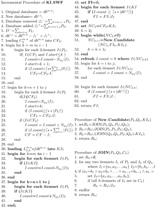
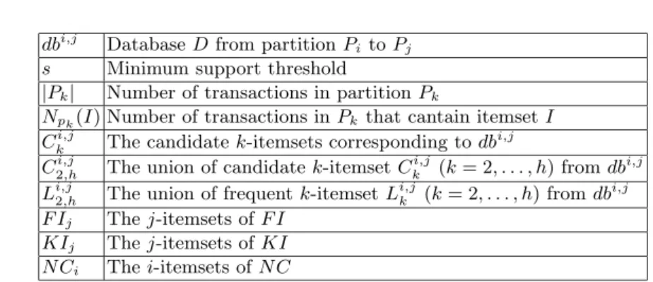
The proposed algorithm, KI SWF (SWF with known itemsets), employs the preprocessing procedure of SWF and extend the incremental procedure as Fig- ure ??. The change portion of the algorithm is presented in bold face. The prepro- cessing procedure is the same as SWF and is omitted here. For ease exposition, the meanings of various symbols used are given in Table 1.
At beginning, we load the cumulative filter CF2 generated in preprocessing procedure (Step 7). From △−, we decrease the counts of itemsets in CF2 and delete non frequent itemsets from CF2with the filtering threshold ⌈s∗D−⌉ (Step 8 to 16). Similarly, we increase the counts of itemsets in CF2 by scanning △+ and delete non frequent itemsets with filtering threshold ⌈s ∗ (D−+ △+)⌉ (Step 17 to 29). After these steps, we get CF2 corresponding to database dbi,j.
Incremental Procedure of KI SWF 1. Original databases = dbm,n; 2. New database= dbi,j;
3. Database removed △−=Pk=m,i−1Pk; 4. Database added △+=Pk=n+1,jPk; 5. D−=Pk=i,nPk;
6. dbi,j= dbm,n− △−+ △+; 7. loading C2m,nof dbm,ninto CF2; 8. begin for k = m to i − 1
9. begin for each 2-itemset I∈Pk; 10. if( I∈CF2 and I.start≤k ) 11. I.count=I.count−Npk(I); 12. I.start=k + 1;
13. if (I.count<⌈s∗Pnt=i|Pt|⌉)
14. CF2=CF2-I;
15. end 16. end
17. begin for k=n + 1 to j
18. begin for each 2-itemset I∈Pk
19. if(I /∈CF2)
20. I.count=Npk(I);
21. I.start=k;
22. if (I.count≥⌈s ∗ |Pk|⌉)
23. CF2= CF2∪I;
24. if (I∈CF2)
25. I.count = I.count + Npk(I); 26. if (I.count≥⌈s ∗Pkt=i|Pt|⌉)
27. CF = CF − I;
28. end 29. end
30. loading Lm,n2,hof dbm,n into KI; 31. begin for k=m to i − 1
32. begin for each itemset I∈Pk
33. if (I∈KI)
34. I.count=I.count-Npk(I);
35. end
36. end
37. begin for k=n+1 to j
38. begin for each itemset I∈Pk
39. if (I∈KI)
40. I.count=I.count+Npk(I);
41. end
42. end;
43. set FI=∅;
44. begin for each itemset I∈KI 45. if (I.count ≥ ⌈s ∗ |dbi,j|⌉) 46. F I = F I∪I;
47. end
48. set N C2=CF2-KI; 49. h = 2;
50. begin while(N Ch6=∅) 51. N Ch+1=New Candidate
(N Ch,F Ih,KIh); 52. h = h + 1;
53. end
54. refresh I.count = 0 where I∈N C2,h; 55. begin for k = i to j;
56. for each itemset I∈N C2,h; 57. I.count = I.count + Npk(I); 58. end
59. begin for each itemset I∈N C2,h; 60. if (I.count≥⌈s ∗ |dbi,j|⌉) 61. F I = F I∪I ; 62. end
63. return F I;
Procedure of New Candidate(Ph,Qh,KIh) 1. setRh=JOIN(Pk,Qh,Ph∪Qh);
2. Rh=Rh∪JOIN(Ph,Ph,Ph∪Qh); 3. Rh=Rh∪(JOIN(Qh,Qh,Ph∪Qh)-KIh); 4. return Rh;
Procedure of JOIN(Ph,Qh,Ch) 1. set Rh=∅;
2. for any two itemsets I1 of Phand I2 of Qh, where I1={a1,a2,. . .,ah} I2={b1,b2,. . .,bh} 4. if (a1=b1∧ a2=b2∧ . . . ∧ ah−1=bh−1∧ ah> bh) 5. set I3={a1,a2,. . .,ah,bh};
6. if (all h-itemsets of I3 are in Ch) 7. Rh= Rh∪I3;
8. endfor 9. return Rh;
Figure 2. Incremental procedure of Algorithm KI SWF
dbi,j Database D from partition Pi to Pj
s Minimum support threshold
|Pk| Number of transactions in partition Pk
Npk(I) Number of transactions in Pk that cantain itemset I Cki,j The candidate k-itemsets corresponding to dbi,j
C2,hi,j The union of candidate k-itemset Cki,j (k = 2, . . . , h) from dbi,j Li,j2,h The union of frequent k-itemset Li,jk (k = 2, . . . , h) from dbi,j F Ij The j-itemsets of F I
KIj The j-itemsets of KI N Ci The i-itemsets of N C
Table 1. Meanings of symbols used
Continually, we load the frequent itemsets that was generated in previous mining task into KI. We check the frequency of every itemset from KI by scanning △−and △+, and put those remaining frequent into F I (Step 30 to 47). Let N C2denotes the itemsets from CF2− KI, i.e. new 2-itemsets that are not frequent in the previous mining procedure and need to be checked by scanning dbi,j. From N C2, we can generate new candidate 3-itemsets (N C3) by JOIN 2- itemsets from N C2, F I2, and KI2. The function New Candidate performs three JOIN operations: N C2⋆N C2, N C2⋆F I2, and F I2⋆F I2. However, if the itemsets are present in KI, they can be deleted since they have already been checked. The third operation is necessary since new candidates may contain supporting (k − 1)-itemsets for a k-itemset to become candidate. We unite the results of the three JOIN operations and get N C3. Iteratively (Step 48 to 53), N C4 can be obtained from N C3, F I3, and KI3. Finally, we scan the database dbi,j and count supports for itemsets in ∪i=2,hN Ciand put the frequent ones to F I (Step 54 to 63).
Sometimes, the size of candidate itemsets in the previous mining procedure is very close to the size of frequent itemsets. If we kept the support counts for all candidate itemsets, and load them to KI at Step 30 in the incremental procedure:
30. Loading C2,hm,n of dbm,n named KI;
The performance, including candidate generation and scanning, can further be speed up. In the next section, we will conduct experiment to compare the original SWF algorithm with the KI SWF algorithms. If the itemsets of KI are the candidate itemsets of the previous mining task, we call this extension CI SWF. If the itemsets of KI are the frequent itemsets of previous mining task, we call this extension FI SWF.
✂✁✄☎✆✝☎✞✟✁✄✄☎✠✁✄
✄
✡✄
✁✄✄
✁✡✄
☛✄✄
☛✡✄
☞✄✄ ✄✌✁✍ ✄✌☞✍ ✄✌✡✍ ✄✌✎✍ ✄✌✏✍
✑✓✒✔✕✖✗✘✘✙✚✛
✜✢✣✤
✥✦✤✧
★ ✩✪✬✫
✫✆✕✩✪✭✫
✮✯✆
✕✩✪✬✫
✰✱✲✳✴✵✳✶✸✷✲✲✳✹✷✲
✲
✺✲✲
✷✲✲✲
✷✺✲✲
✱✲✲✲
✱✺✲✲ ✲✻✷✼ ✲✻✽✼ ✲✻✺✼ ✲✻✾✼ ✲✻✿✼
❀✟❁❂❃❄❅❆❆❇❈❉
❊❋●❍
■❏❍❑
▲ ▼◆✬❖
❖✴❃▼◆✬❖
P◗✴
❃▼◆✭❖
(a)
❘✂❙❚❯❱❲❯❳✓❙❚❚❯❨❙❚❬❩❬❭❪❫❴❵❛❛❜❝❞❡❚❢❙❣
❤
✐❤
❥❤❤
❥✐❤
❦❤❤
❦✐❤
❧❤❤ ♠♥♣♦ ♦qr♠♥♣♦ s◗qr♠♥♣♦
t✉✈✇
①②✇③
④ ⑤⑥⑦⑧⑨⑦⑩⑦❶⑦⑤❷⑨❶❸❹❺❻
⑥⑦⑧⑨❹⑥⑦⑩❷❼❷⑧❷❽⑦⑩❹❾⑧
⑥⑦❿⑥➀❿⑦⑩❷⑧❷➁✟⑤➀➂➂❾❽⑩
⑦⑨⑨➂⑦❽⑩❹⑩❹❾⑧⑤
⑨❷❿❷⑩❷➂⑦❽⑩❹⑩❹❾⑧⑤ ➃➄➅➆➇➈➆➉✸➊➅➅➆➋➊➅➍➌✟➎➏➐➑➒➓➓➔→➣↔➅↕➊➙
➅
➛➅➅
➊➅➅➅
➊➛➅➅
➄➅➅➅
➄➛➅➅ ➜➝✬➞ ➞➇➐➜➝✬➞ ➟◗➇➐➜➝✬➞
➠➡➢➤
➥➦➤➧
➨ ➩➫➭➯✯➲➭➳➭➵➭➩➸➲➵➺➻➼➽
➫➭➯➲➻➫➭➳➸➾➸➯➸➚➭➳➻➪➯
➫➭➶➫➹➶➭➳➸➯➸➘✟➩➹➴➴➪➚➳
➭➲➲➴➭➚➳➻➳➻➪➯➩
➲➸➶➸➳➸➴➭➚➳➻➳➻➪➯➩
(b)
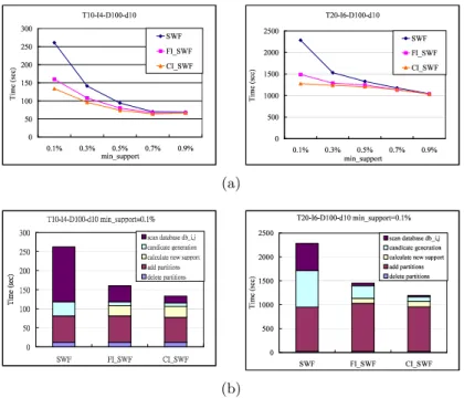
Fig. 3. Execution time vs. minimum support
4 Experiments
To evaluate the performance of FI SWF algorithm and CI SWF algorithm, we preformed several experiments on a computer with a CPU clock rate of 800 MHz and 768 MB of main memory. The transaction data resides in the FAT32 system and is stored on a 30GB IDE 3.5 drive. The simulation program was coded in C++. The method to generate synthetic transactions we employed in this paper is similar to the ones used in [4, 9, 3]. The performance comparison of SWF, FI SWF, and CI SWF is presented in Section 4.1. Section 4.2 shows the memory required and I/O cost for the three algorithms. Results on scaleup experiments are presented in Section 4.3.
4.1 Running Time
First, we test the speed of the three algorithms, FI SWF, CI SWF, and SWF. We use two different datasets, T 10 − I4 − D100 − d10 and T 20 − I6 − D100 − d10, and set N =1000 and |L|=2000. Figure 3(a) shows the running time of the three algorithms as the minimum support threshold decreased from 1% to 0.1%. When the support threshold is high, the running times of three algorithms are similar. Because there are only a limited number of frequent itemsts produced. When
the support threshold is low, the difference in the running time becomes large. This is because when the support threshold is low (0.1%), there are a lot number of candidate itemsets produced. SWF scanned the total databases dbi,j for all candidate itemsets. FI SWF scanned dbi,j for the candidate itemsets that are not frequent in previous mining tasks or not present in previous mining tasks. CI SWF scanned dbi,j only for the candidate itemsets that are not present in previous mining tasks. The details of the running time of three algorithms are shown in Figure 3(b). For SWF, the incremental procedure includes four phase: delete partitions, add partitions, generate candidates and scan database dbi,j. For FI SWF and CI SWF, they take one more phase to count new supports for known itemsets. The time for deleting or add partitions is about the same for three algorithms, while SWF takes more time to generate candidates and scan database.
4.2 The Memory Required and I/O Cost
Intuitively, FI SWF and CI SWF require more memory space than SWF because they need to load the itemsets of the previous mining task and CI SWF needs more memory space than FI SWF. However, the maximum memory required for these three algorithms are in fact the same. We record the number of itemsets kept in memory at running time as shown in Figure 4(a). The dataset used was T10 − I4 − D100 − d10 and the minimum support was set to 0.1%. At beginning, the memory space used by SWF algorithm was less than the others, but the memory space grew significantly at the candidate generation phase. The largest memory space required at candidate generation is the same as that used by CI SWF and FI SWF. In other words, SWF still needs memory space as large as CI SWF and FI SWF. The disk space required is also shown in Figure 4(a), where “CF2+ KI” denotes the number of itemsets saved for later mining task. From this figure, CI SWF require triple disk space of SWF. However, frequent itemsets are indeed by-product of previous mining task.
To evaluate the corresponding cost of disk I/O, we assume that each read of a transaction consumes one unit of I/O cost. We use T 10 − I4 − D100 − d10 as the dataset in this experiment. In Figure 4(b), we can see that the I/O costs of FI SWF and CI SWF were a little higher than SWF. This is because that FI SWF and CI SWF must scan the changed portions of the database to update the known itemsets’ supports.
4.3 Scaleup Test
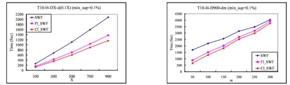
Continuously, we test the scaleup ability of FI SWF and CI SWF with large databases. We conduct two experiments. In the first experiment, we use T 10 − I4−DX −d(X ∗0.1) as the dataset, where X represents the size of the databases and the changed portions are 10 percents of the original databases. We set X = 300, 600, 900 with min support=0.1%. The result of the second experiment is shown in Figure 5(a). We find the the response time of these two algorithms were linear to the size of the databases. In the second experiment, we use T 10 −
➷✯➬➮➱✃❐➱❒✟➬➮➮➱❮➬➮
➮
❰➮➮➮
➬➮➮➮➮
➬❰➮➮➮
Ï➮➮➮➮
Ï❰➮➮➮
Ð➮➮➮➮
Ð❰➮➮➮
❐➮➮➮➮ ÑÒ✬Ó Ó✃ÔÑÒ♣Ó Õ✃ÔÑÒ✬Ó
Ö×Ø
×
ÙÚ
Û×Ü
Ý
ÞßÛÝàÚÝ ÛÚ
áâãâäâ
åæçäèäèéê
æáá
åæçäèäèéê
ëæêáèëæäâ
ìâêâçæäèéê
íîïðñ✯ò
ó➍ôõö÷øöù✸ôõõöúôõ
õ
ûõ
øõ
üõ
ýõ
ôõõ
ôûõ
ôøõ
ôüõ õþôÿ õþÿ õþ✁ÿ õþ✂ÿ õþ✄ÿ
☎✝✆✞✟✠✡☛☛☞✌✍
✎
✏ ✑✒✓✔
✕
✖ ✗✘✙
✚ ✛✜✣✢
✢✤✥✛✜✦✢
✧★✤✥✛✜✣✢
(a) Memory required at each phase (b) I/O cost for three algorithms
Fig. 4. Memory required and I/O cost
✩✫✪✬✭✮✯✭✰✲✱✲✭✳✴✬✵✪✱✲✶✴✷✝✸✹✺✻✼✽✾✬✵✪✿✝✶
❀
❁❀❀
❂❀❀
❃❀❀
❄❀❀
❅❀❀❀
❅❁❀❀
❅❂❀❀
❅❃❀❀
❅❄❀❀
❁❀❀❀
❁❁❀❀ ❆❇❇ ❈❇❇ ❉❇❇ ❊❇❇ ❋❇❇
●
❍
■❏
❑
▲▼❑◆
❖ P◗❙❘
❘❚❯P◗❙❘
❱❚❯P◗❲❘
❳✫❨❩❬❭❪❬❫❵❴❩❩❬❛❜❞❝❜✝❡❢❣❤✐❥❦❩❧❨♠✝♥
♦
♣♦♦
q♦♦♦
q♣♦♦
r♦♦♦
r♣♦♦
s♦♦♦
s♣♦♦
t♦♦♦
t♣♦♦ ♣♦ q♦♦ q♣♦ r♦♦ r♣♦ s♦♦
✉
✈✇①②
③ ④②⑤
⑥ ⑦⑧❲⑨
⑨⑩❶⑦⑧❲⑨
❷⑩❶⑦⑧❲⑨
(a) Execution time vs. the database size (b) Execution time vs. the changed portions
Fig. 5. Scalable test
I4 − D900 − dm as the dataset and set min support to 0.1%. The value of m is changed from 100, 200, to 300. The result of the this experiment is shown in Figure 5(b). As △+ and △− became larger, it requires more time to scan the changed partitions of the dataset to generate CF2 and calculate the new supports. From this two experiments, we can say that FI SWF and CI SWF have the ability of dealing with large databases.
5 Conclusion
In this paper, we extend the sliding-window-filtering technique and focus on how to use the result of the previous mining task to improve the response time. Two algorithms are proposed for incremental mining of frequent itemsets from up- dated transaction database. The first algorithm FI SWF (SWF with Frequent Itemset) reuse the frequent itemsets (and the counts) of previous mining task as FUP2 to reduce the number of new candidate itemsets that have to be checked.
The second algorithm CI SWF (SWF with Candidate Itemset) reuse the can- didate itemsets (and the counts) from the previously mining task. From the experiments, it shows that the new incremental algorithm is significantly faster than SWF. In addition, the need for more disk space to store the previously discovered knowledge does not increase the maximum memory required during the execution time.
References
1. R. Agarwal, C. Aggarwal, and V.V.V Prasad. A tree projecction algorithm for generation of frequent itemsets. Journal of Parallel and Distributed Computing (Special Issue on High Performance Data Mining), 2000.
2. R. Agrawal, T. Imielinski, and A. Swami. Mining association rules between sets of items in large databases. In Proc. of ACMSIGMOD, pages 207–216, May 1993. 3. M.-S. Chen C.-H. Lee, C.-R. Lin. Sliding-window filtering: An efficient algorithm
for incremental mining. In Intl. Conf. on Information and Knowledge Management (CIKM01), pages 263–270, November 2001.
4. D. Cheung, J. Han, V. Ng, and C.Y. Wong. Maintenance of discovered association rules in large databases: An incremental updating technique. In Data Engineering, pages 106–114, February 1996.
5. D. Cheung, S.D. Lee, and B. Kao. A general incremental technique for updaing discovered association rules. In Intercational Conference On Database Systems For Advanced Applications, April 1997.
6. J. Han and J. Pei. Mining frequent patterns by pattern-growth: Methodology and implications. In ACM SIGKDD Explorations (Special Issue on Scaleble Data Min- ing Algorithms), December 2000.
7. J. Han, J. Pei, B. Mortazavi-Asl, Q. Chen, U. Dayal, and M.-C. Hsu. Freespan: Frequent parrten-projected sequential pattern mining. In Knowledge Discovery and DAta Mining, pages 355–359, August 2000.
8. J.-L. Lin and M.H. Dumham. Mining association rules: Anti-skew algorithms. In Proc. of 1998 Int’l Conf. on Data Engineering, pages 486–493, 1998.
9. J.-S Park, M.-S Chen, and P.S Yu. Using a hash-based method with transaction trimming for minng association rules. In IEEE Transactions on Knowledge and Data Engineering, volume 9, pages 813–825, October 1997.
10. J. Pei, J. Han, and L.V.S. Lakshmanan. Mining frequent itemsets with convertible constraints. In Proc. of 2001 Int. Conf. on Data Engineering, 2001.
11. A. Savasere, E. Omiecinski, and S. Navathe. An efficient algorithm for mining association rules in large databases. In Proc. of the 21th International Conference on Very Large Data Bases, pages 432–444, September 1995.
12. A. Veloso, B. Possas, W. Meira Jr., and M. B. de Carvalho. Knowledge manage- ment in association rule mining. In Integrating Data Mining and Knowledge Man- agement, 2001.
13. Z. Zhou and C.I. Ezeife. A low-scan incremental association rule maintenance method. In Proc. of the 14th Conadian Conference on Artificial Intelligence, June 2001.