Between Alpha and Beta:
Modeling The Impact of Regulatory Constraints
on the Hedge Fund Industry
Anna Ilyina and Roberto Samaniego* June 2010
Abstract
Decreasing returns to scale and scarcity of manager talent are important determinants of the dynamics of the portfolio management industry. In a calibrated model of the hedge fund industry, we explore the implications of these features for the equilibrium response of the industry to regulatory change. An increase in due diligence costs reduces the number of active hedge funds, while leaving industry capital under management unaffected. By contrast, a leverage limit decreases hedge funds’ capital under management significantly – even when small funds are exempt – and may lead certain hedge fund styles to become non-viable.
JEL Codes: G11, G23, L25, L84.
Keywords: Portfolio management, hedge funds, diminishing returns, alpha, manager talent, leverage caps, due diligence costs, financial regulation, industry dynamics.
* Roberto Samaniego (corresponding author): George Washington University, Department of Economics, 2115 G St NW Suite 340, Washington DC, 20052. Email: [email protected]. Anna Ilyina: International Monetary Fund, Monetary and Capital Markets, 700 19th St NW,
I. INTRODUCTION
The regulation of the financial sector is a topic that has gained prominence in the wake of the subprime crisis and the subsequent global recession. Proposals include the expansion of the “perimeter of regulation” to cover lightly regulated entities such as hedge funds, using measures such as new reporting requirements and limits on leverage. An assessment of the long-run impact of subjecting hedge funds to tighter regulation requires a quantitative model that captures salient features of the industry that would affect its equilibrium response – for example, via changes in industry composition, changes in capital under management and changes in profitability. This paper develops such a model.
Recent work has identified fund size and scarcity of asset manager talent as two important determinants of the returns to actively managed funds. This is in contrast to standard models of asset management, which assume that portfolio returns are driven by the statistical
properties of the underlying assets. Berk and Green (2004) argue that differences in the quality of asset managers and decreasing returns to fund size can reconcile a number of empirical regularities in portfolio management with efficient market theory and rational expectations. In addition, several authors find evidence supporting the presence of decreasing returns to scale in the hedge fund industry.1 Hence, decreasing returns and limited talent are likely to be critical determinants of the response of the hedge fund industry to any changes in regulatory constraints – particularly since proposed changes directly impact the size of hedge fund investments (e.g. caps on leverage) and the composition of the hedge fund industry (e.g. higher fixed costs, such as the cost of due diligence). In spite of work underlining the
importance of decreasing returns and limited talent for the behavior of the asset management industry, the implications of these features for the response of the industry to changes in regulation have not been explored.
We develop a theoretical model in which the size and composition of the hedge fund industry are endogenous. The model features a set of potential fund managers, but which of them operate hedge funds in equilibrium depends on their profitability. In turn, profitability hinges both on talent and on luck. We estimate the key parameters of the model, and calibrate the model to assess the impact on the hedge fund industry of changes in the regulatory
environment, including an increase in the cost of due diligence, an increase in the cost of leverage, and a cap on leverage ratios. These are among the regulatory initiatives that are currently being discussed – see ECB (2006), FSA (2009) and Malcolm et al (2009).
In the model, hedge funds differ in terms of talent, and experience shocks to their returns. At any date they may raise funds and place them in an investment strategy, the returns to which depend on fund size, on talent, and on the shocks (which we will refer to as “luck”). The equilibrium industry size is determined by the presence of negative spillovers across funds. This captures the notion that hedge funds may engage in similar strategies, so that increased investments in a given hedge fund lower the returns of other funds. For example, to the extent that some hedge funds earn profits from arbitrage, the size of their positions could
1
affect prices in the mis-priced markets and lead to lower returns (Perold and Salomon (1991)) – and the presence of other managers following the same strategy could have similar effect.2 Our model builds on the Hopenhayn (1992) industry framework with entry and exit, adapted to match specific features of hedge funds – for example, the presence of cross-fund
spillovers, and of leverage. In our paper leverage is capped exogenously, either by best-practice norms or by the regulator, as in the entrepreneurial model of Evans and Jovanovic (1989). Aghion et al (1999) provide a theoretical foundation for fixed leverage ratios, showing that such a borrowing limit can emerge as an equilibrium outcome of a game between borrowers and creditors in an environment with limited commitment in which borrowers may divert funds at a cost.
In order to calibrate the model, we estimate a reduced form panel specification that maps into the model parameters, using data on hedge fund capital under management and returns. The econometric model decomposes hedge fund returns into effects due to size, talent and luck. We identify manager talent using fund-level fixed effects. The identification of managerial talent with a fund-specific fixed effect is consistent with Lo (2008), who argues that the manager essentially is the fund, and with Liang and Park (2010), who find that the exit of a hedge fund is often tied to the career decisions of the fund manager. Thus, we can identify the existence and distribution of manager talent though its permanent effect on returns.3 It should be noted that our specification allows luck to be serially correlated, so our model nests the possibility that there are no fixed effects and only temporary (thought persistent)
differences in returns.
Using these estimates, we calibrate the theoretical model and use it to assess the impact on the industry of an increase in entry costs, of an increase in the borrowing cost, and of an imposition of leverage limits. Our simulations show that the interaction of limited talent and decreasing returns are central to the response of the industry to regulatory change. The main results are as follows:
• A significant increase in entry costs has a large impact on the number of hedge funds, but little impact on the total industry capital under management and profits.
2
Getmansky (2004), Khandani and Lo (2007) and Chan et al (2007) all mention the possibility of “congestion” of hedge fund positions. An example is the October 28, 2008 spike in the Volkswagen share price as hedge funds closed large short positions that exceeded the value of outstanding Volkswagen shares – leading
Volkswagen to be (briefly) the largest company in the world by market value, and generating significant losses for the hedge funds involved.
3
This is because the increase in operating costs raises the bar on the profitability required for hedge funds to enter and survive: however, this would affect mainly the funds with the lowest manager talent, which comprise a small fraction of total industry capital under management.
• By contrast, an increase in the cost of borrowing or the imposition of a leverage limit at a level below the current industry norms can have a large impact on industry capital under management and profits. This is because a leverage limit lowers the profits that funds can generate with a dollar of capital – the “productivity” of the hedge fund. This does not affect rates of return, because lower profitability is offset by hedge funds optimally reducing their portfolios. Furthermore, exempting funds that are smaller than a certain size threshold from leverage limit does not change this result, but by weakening the negative spillover across the funds, it may encourage the entry of hedge funds that in the absence of such limits would have been unprofitable, and hence, may lead to lower average quality of funds.
The paper has several contributions. First and foremost, the policy implications of talent scarcity and decreasing returns to scale in the asset management industry have not been explored before – in spite of the relevance of these features for the evaluation of the regulation of the industry. Second, the implications of the specific policy changes we contemplate have not been explored in an equilibrium context. There exist studies of the impact of new regulations on hedge funds by regulatory agencies or commissioned by such agencies (e.g. ECB (2006), Malcolm et al (2009) and FSA (2009, 2010)), but these studies do not model the equilibrium response of the industry to changes in regulation.
Third, our calibration procedure can be interpreted as an estimation of a version of the Hopenhayn (1992) framework, for the case of the hedge fund industry. We argue that this framework is appropriate for the asset management industry and, to our knowledge, this is the first application of this framework for policy analysis in the context of financial markets.4 Fourth, we arguably provide more accurate estimates of the impact of size on returns in the hedge fund industry. We cannot calibrate our model using existing estimates of the impact of size on hedge fund returns because prior studies do not jointly estimates the impact of size and talent on hedge fund returns. In a world of non-decreasing returns to scale, heterogeneity of manager talent is of no consequence, since all resources could simply be allocated towards the best manager. Conversely, decreasing returns to fund size need not limit profits if the pool of manager talent is unlimited, as investors could increase returns by spreading their assets more thinly over a larger number of managers. Thus, any attempt to model
theoretically or econometrically one feature requires modeling the other. Our quantitative results show that the response to regulation of the asset management industry depends very much on the interaction of size and talent.
4
Section II provides a summary of the related literature. Section III describes the model, and Sections IV calibrates the model parameters, and discusses the empirical relevance of the model framework for the case of hedge funds. Section V assesses the impact of regulatory changes on the hedge fund industry and discusses extensions. Section VI concludes.
II. BACKGROUND ON HEDGE FUNDS
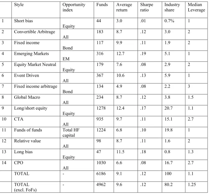
A. The Hedge Fund Industry: some Stylized Facts
We begin with a discussion of some distinguishing features of the hedge fund industry that motivate our modeling approach. Related discussions may be found in Financial Stability Forum (2000), Getmansky (2004), Malkiel and Saha (2005), and CISDM (2006).
Several features of hedge funds distinguish them from more traditional asset managers (such as mutual funds), and are important for modeling hedge fund industry dynamics:
• Hedge fund strategies may not be “scalable.” Many hedge fund investment styles exploit market imperfections, such as arbitrage opportunities or profitable
opportunities in less liquid markets: see Ammann and Moerth (2005) and Lo (2008). If so, sufficiently large positions at a given hedge fund would erode the market conditions that the hedge fund strategy is designed to exploit (e.g. see Perold and Salomon (1991) and Koutsougeras (2003)).The size effect could also be due to administrative costs that increase more than proportionately with capital under management, as in Ammann and Moerth (2005). Lucas (1978) suggests that
managers may have limited supervisory resources. The fact that hedge funds tend to close down to new investors whenever they reach certain size is arguably evidence of decreasing returns, with Ackermann et al (1999) and others even arguing that each hedge fund has an “optimal size”.
• There are negative externalities across hedge funds. To the extent that hedge funds exploit market imperfections such as arbitrage opportunities, their profits may be eroded if the positions of other funds following similar investment strategies hare large. There is indeed evidence that hedge fund investment strategies can overlap, and that this reduces profits: see Khandani and Lo (2007) on profit spillovers across “quant” hedge funds in 2007. Getmansky (2004) argues that returns are lower in fund styles with more intense competition, and Chan et al (2007) argue that large inflows into the hedge fund industry were one cause of deteriorating returns in 2004.
• The fund manager’s “talent” is a key determinant of hedge fund returns. Hedge funds derive a significant part of their return from active portfolio management; see Ackermann et al (1999). Hedge fund performance is commonly linked to “alpha”, interpreted as manager talent or as the quality of the manager’s investment strategy. 5
5
• Talent is scarce. Entry costs are far lower than profits at the average hedge fund. Brown et al (2008b) estimate the typical due diligence cost to the investor of
contracting a hedge fund to be in the range $50,000-100,000. Strachman (2007) also reports the cost of starting a hedge fund to be about $50,000. By contrast, the mean assets under management at hedge funds is over $100,000,000 and mean annual return is about 9%, so mean annual profits should be over $9,000,000. This suggests that there may be more important constraints on industry growth than entry costs: instead, the size of the hedge fund industry is limited by the availability of sufficiently talented fund managers.
• Exit is common, and often sudden. Liang and Park (2010) find that about a third of exits can be attributed to low fund profitability, whereas two thirds of exits occur for other reasons, including changes in the career concerns of the fund manager and operational risks (e.g. fraud).6 Indeed, Lo (2008) argues that in essence the fund manager is the fund, so his/her departure for any reason almost certainly marks the end of the hedge fund. Thus, many exits are due to factors unrelated to low
profitability. As for the remainder, Getmansky et al (2004) find that profits at hedge funds tend to deteriorate within 12 months before exit, though not obviously before.
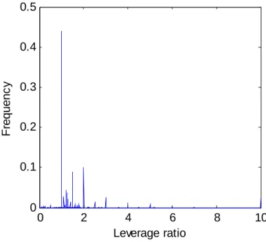
• Leverage is common, but varies relatively little across funds. Figure 1 shows reported leverage from the CISDM (2006) database. The distribution is degenerate: about 45 percent of all hedge funds in the database report leverage equal to one – meaning that they typically borrow an amount roughly equal to their capital under management. Independently, the UK Financial Services Authority (2009, 2010) also finds that reported values of leverage cluster around one. In fact, most responses are integers and, if we round all responses to the nearest integer, 65% of hedge funds report leverage of one. Some view differences in leverage as being, in large part, a function of the hedge fund style (e.g., Schneeweis et al (2005) and Managed Funds Association (2009)) and, indeed, a median regression of leverage against style dummies using CISDM (2006) data yields significant coefficients for all styles, (a median regression is appropriate because there are some significant outliers, and because leverage is often reported as an integer: see Figure 1). Thus, the hedge fund’s level of leverage is best thought of as a given (possibly style-specific) parameter.
6
With these stylized facts in mind, we construct a theoretical model of the hedge fund industry. We estimate the parameters of the model using panel regression analysis. We use the estimates to calibrate the theoretical model, and apply the model to quantify the long-run impact on the hedge fund industry of several regulatory restrictions that are currently under consideration.
Figure 1: Distribution of leverage ratios, CISDM database.
The leverage ratio is defined as the ratio of borrowed funds to capital.
0 2 4 6 8 10
0 0.1 0.2 0.3 0.4 0.5
F
re
que
nc
y
Leverage ratio
B. Regulatory Initiatives for the Hedge Fund Industry
Hedge funds face few investment restrictions, and those they do face are typically determined by their own internal risk management guidelines and “best practice” norms. See, for
What are the main regulatory changes under consideration and what is their likely impact?
• Imposing additional reporting requirements. Brown et al (2008a) study the impact on hedge funds and investor behavior of the (subsequently repealed) requirement that all hedge fund managers register as investment advisors with the United States Securities and Exchange Commission. They find that imposing this requirement did not lead hedge fund managers to provide any substantive information to investors in addition to what was already made available to them. Thus, we focus on quantifying the costs associated with the imposition of additional reporting requirements on hedge funds, in the form of entry and operating costs.
• Imposing leverage limits. The justification for leverage limits is that they would reduce the hedge funds’ contribution to systemic risk. The FSA (2010), however, concludes that there is no threat from hedge funds to the banking system based on current levels of leverage. In addition, Chan et al (2007) argue that the main systemic threat coming from hedge funds stems from an across-the-board unwinding of
positions due to lack of liquidity. While there does not seem to be a clear evidence to suggest that there is any benefit from leverage caps, Malcolm et al (2009), e.g., argue that leverage caps would reduce profits and the number of hedge funds if the limits are much tighter than current best practice. In this paper, we focus on quantifying the potential impact of leverage limits (as well as size-contingent leverage limits) on the number funds and on total capital under management of the hedge fund industry.
• Increasing the cost of leverage. Increases in the cost of borrowing might lead to a shrinking of the industry. This could happen, for example, because regulators might require other financial intermediaries to raise the margin requirements for hedge funds. As we have seen during the recent crisis, the sharp 1.2 percent increase in 3-month LIBOR in October 2008 coincided with a significant reduction in the number and size of hedge funds across the board, though clearly not all of the impact could be attributed to a single cause. In what follows, we consider the impact of an increase in the cost of leverage on the number of funds and on total capital under management of the hedge fund industry.
III. THEORETICAL MODEL
A. Basic Structure
The model assumes a single hedge fund style. This enhances tractability, but does not affect the main results of the paper, as discussed in Section VI.
There is a continuum of risk neutral investors,7 each of whom invests in hedge funds and decides on the capital q to be allocated to each. At any point in time, the investors may decide to close a hedge fund, if its expected profitability is too low. The investors may also activate hedge funds from the distribution of potential fund managers, at a cost ce.
B. Hedge Funds
Time is discrete, and there is no aggregate uncertainty. In any period t, each hedge fund i is characterized by a stochastic return factor εit (luck), and a deterministic factorμi (talent).
There is a distribution ξt over potential fund managers and their current realizations of luck, as well as their incoming assets under management: the distribution may change over time as managers enter, exit, experience changes in luck, or change their capital. Define Θ as the transition function forξt: Θ is endogenous, and is determined in equilibrium by the process
εit as well as by flows of potential managers in and out of the industry.
Luck εit is a random variable that follows a Markov process given by a distribution
functionF
(
εi t, 1+ |εit)
. F has an ergodic distribution Fe. When an investor chooses to activate a fund at time t, the hedge fund’s initial value of εit is drawn from a distribution G: before activation we assume ε= -∞. The range of εitis assumed to be bounded. Both talent and luck are observable.Each period a volume of potential fund managers becomes available, each one with a value of talent drawn from a distribution ζ. The volume and distribution of entrants is exogenous, capturing the notion that manager talent is a scarce resource (we discuss relaxing this assumption in Section V). Which hedge funds are active is determined in equilibrium, however. There is a cost to the investor ce of activating a fund, representing the cost of due diligence, and which is imposed by regulators. Firms with an expected value below ce are not activated. Define *
t
μ as the talent level below which fund managers do not receive capital to activate a hedge fund. There is also a per-period cost κ that the investor must pay to keep the fund active. This is the cost of ongoing due diligence.
Liang and Park (2010) distinguish between two different sources of exit. First, funds may close because of exogenous reasons unrelated to firm profitability, in which case they exit the pool of potential fund managers. This occurs in the model with probability e. We interpret this as a change in the manager’s career concerns, as the manager’s retirement, or as closure due to legal problems. Second, funds may close due to the lack of profitability of their strategy, in which case the managers also leave the industry. We allow this to happen in the model in two ways. In any period the investor may liquidate the position and shut down the
7
fund if the fund is unprofitable. In addition, the fund’s strategy may cease to be profitable exogenously with probability s. This is interpreted as the obsolescence of the fund manager’s investment strategy or talent value (for example, due to its revelation and
imitation by other types of financial intermediaries, who may engage in similar strategies: see Chan et al (2007)).8 Thus, fund managers exit exogenously each period with probability =
e + s. Allowing > 0 ensures that all hedge funds close in finite time with probability one, and represents a lower bound on the exit rate of funds in the industry.
The hedge fund earns revenues for the investor by using investor contributions to open an investment position. The hedge fund can invest funds obtained by raising capital or via leverage. The quantity mi,t-1 is the value of the fund’s investments. If the hedge fund’s capital is qi,t-1, and it borrows an additional proportion x of qi,t-1, then the fund’s position is
mi,t-1 = qi,t-1(1+x). (1) The revenue from the investment mi,t-1 is equal to:
(
i t, 1, t 1, i, it)
0f m − M− μ ε ≥ (2)
The revenue f depends on the size of investment position mi,t-1, and also on Mt-1 which is the total size of positions of all funds in a given style. Having observed f, the investor decides whether to allocate funds mi,t ≥ 0 to the hedge fund for the following period.
Let p≥1 be the cost of raising funds. We define p in a simple way so as to distinguish between capital and debt, while allowing us to abstract from any particular theory of capital structure. To raise a dollar of capital costs 1+k dollars. This represents foregone consumption plus a premium k to open a position. Funds may also use leverage,9 and the cost of leverage is c, where c<k. This last assumption implies that hedge funds would prefer to invest only using borrowed funds. However, we also assume a maximum leverage ratio x, imposed either by “best practice” guidelines or by the regulator (see Section II).We define the leverage ratio x as the ratio of borrowed funds to capital q. This is the definition used by many hedge fund data providers, including CISDM. Thus, the total cost of a position mit is qit(1+k)+cxqit. The cost of funding a dollar of capital is p≡ + +
( )
1 k xc. The assumption of an exogenously fixed leverage ratio is a common way of modeling credit constraints, as in Evans and Jovanovic (1989), and Aghion et al (1999) provide a micro-foundation for such a credit constraint based on the borrower being able to divert the profits of the venture, at a cost. Thus, our leverage ratio can be interpreted either as an institutionally imposed value, or as an equilibrium outcome in an environment with limited commitment.8
As noted, Getmansky et al (2004) find that a link between deteriorating performance and exit appears within 12 months of the exit itself. Later, we identify a period in the model with one year, to avoid having to model a distinct period of several months over which profits deteriorate.
9
Recalling Section II, the fact that leverage ratios are so concentrated suggests that the mechanisms of theories that endogenize the cross-sectional variation in capital structure are not appropriate for the case of hedge funds.For example, a motivation for Cooley and Quadrini (2001) is that, in industry, leverage and size are thought to be negatively related, whereas in the case of hedge funds we find that the correlation in CISDM (2006) data is positive (9%) and has no statistical significance when conditioning on style dummies. 10 The same is true in a median regression, or with bootstrapped standard errors, procedures which are less sensitive to outliers. This is what motivates our approach to modeling leverage ratios. At a continuing fund, let distributions to the investor di,t equal revenues minus costs and capital for the subsequent period, assuming the hedge fund does not close:
(
)
, , 1, 1, , ,
i t i t t i it i t
d = f m − M − μ ε −pq −κ (3)
If di,t >0, then the hedge fund is paying out distributions. If di,t <0, then the hedge fund is raising additional capital from the investor.
There are decreasing returns to scale, so that f1 > 0, f11 < 0. We also assume
that f
(
0,Mt−1,μ εi, it)
=0. When a manager enters the industry, qi,t-1=0, and in order to activate the hedge fund, the manager must raise initial capital.We assume that f2 < 0, so that higher assets under management in the style lower the returns to all hedge funds in that style. We further assume that f m
(
i t, 1− , 0,μ εi, it)
= ∞ and(
i t, 1, , i, it)
0f m − ∞ μ ε = . These assumptions ensure equilibrium existence.
Finally, returns also depend upon talent μi and on luck εit, so that f3 > 0 and f4 > 0.
The investor maximizes expected discounted distributions di,t from the hedge fund. We can represent the hedge fund manager’s problem recursively (the existence of a unique recursive representation of the hedge fund’s problem follows from standard results in dynamic
programming: see Stokey et al (1989)). Consider at the beginning of period t a hedge fund with assets under management mi,t-1, talent μi, and a realization of luck εit, in an industry
with total capital Qt-1 = Mt-1/(1+x). Define V q
(
i t, 1− ,Qi t, 1−,μ εi, it)
as the value of the expected discounted profits of investing in such a hedge fund.10
Furthermore, define V qc
(
i t, 1−,Q, 1t− ,μ εi, it)
to be the value of investing in the fund assuming that it continues in operation, and let V qe(
i t, 1− ,Qi t, 1− ,μ εi, it)
be the value to the investor of investing in a fund assuming it is not going to continue. Then, the value of operating a hedge fund equals the maximum of continuing or closing the hedge fund.(
)
{
(
)
(
)
(
)
(
)
}
, 1 , 1 , 1 , 1
, 1 , 1
, 1 , 1
max , , , , , , ,
, , ,
1 , , , .
e i t i t i it e i t i t i it
i t i t i it
c i t i t i it
V q Q V q Q
V q Q
V q Q
μ ε δ μ ε
μ ε
δ μ ε
− − − −
− −
− −
=
+ − (4)
Then, the continuation value of the fund is:
(
)
(
)
( )
( )
(
)
,
, 1 , 1 , , 1
, , , 1 1
1
, , , max , , ,
1 . .
1 , 1 , ,
i t
c i t i t i it i t it it i i t
q
i t i t i t t i it
V q Q d E V q Q
r s t
d pq f x q x Q
ε
μ ε μ ε
κ μ ε
− − + − − ⎧ ⎫ = + ⎨ ⎬ + ⎩ ⎭ + + ≤ + + (5)
where the expectation is taken with respect to the distribution of future luck conditional on current luck (distribution F). The solution to this problem qi t*, is given by:
( ) ( )
(
( ) ( )
*)
(
)
1 , , 1 , 1 , 1
1 1 1 i t, 1 t, i, i t i t | it i t
p + = +r x
∫
f +x q +x Q μ ε + F ε + ε dε + (6)so that the optimal fund size depends on the manager’s talent, on the current realization of luck, and on capital at other hedge funds.
The value to the investor of closing the fund is:
(
, 1, , 1, ,)
(
( )
1 , 1, 1( )
, 1, ,)
e i t i t i it i t i t i it
V q − Q − μ ε = f +x q − +x Q − μ ε (7)
Thus, the investor allocates * ,
i t
q to the hedge fund each period, unless the expected return is so low that it is cannot cover the recurring fixed costs. This specification assumes that there is a one-period delay required to open a new hedge fund: this assumption is realistic but not necessary. There is a non-negativity constraint on qi,t, but not on di,t.
Equations (4) – (7) should be interpreted as follows. Having made an investment of qi,t-1 in the previous period, at the beginning of period t the returns f are realized. Then, the investor decides whether or not to close the fund: if it closes then di,t = f. In addition, with
(
)
(
( )
( )
)
(
)
(
)
, 1 , 1 , 1 1
, 1
, , , 1 , 1 , ,
1
1 max 0, max , , , .
1
it
i t i t i it i t t i it
it it t i i t
q
V q Q f x q x Q
pq E V q Q
r ε
μ ε μ ε
δ κ μ ε
− − − − + = + + ⎧ ⎡ ⎤⎫ + − ⎨ ⎢− − + ⎥⎬ + ⎣ ⎦ ⎩ ⎭ (8)
C. Equilibrium
The model distinguishes between the distribution of active fund managers and the distribution of potential fund managers. The equilibrium distribution of potential fund managers is exogenous, and can be defined using the results of Hopenhayn and Prescott (1992). The distribution of active fund managers is related, but is truncated. The truncation rule is complex: there is a talent threshold μt* below which firms do not enter, but after entering they may exit as a result of bad luck. The luck threshold below which an agent of a given talent exits isε μt*( ).
At the beginning of any period a hedge fund takes as given the vector11
(
)
1, ,
it it i it
x = q − μ ε .
Let X = ℜ ×ℜ+ 2 be the set of possible values of the vector xit . Let ξt:X
+
→ ℜ be the measure over types of funds at the beginning of date t.12 Recall that returns (and the economy’s state) also depend on Qt-1, which is drawn from the real numbers. Definition 1: An equilibrium is a sequence
{
* *( )
}
0
, , ,
t Qt t t t
ξ μ ε μ ∞= and decision rules such that the sequence
{
* *( )
}
0
, , ,
t Qt t t t
ξ μ ε μ ∞= results from optimal behavior, and the behavior is optimal
at each fund given the sequence
{
* *( )
}
0
, , ,
t Qt t t t
ξ μ ε μ ∞= . Specifically,
(
*)
( )
0, t, t, it it e
V Q μ ε dG ε =c
∫
,∫
V(
0,Qt, ,μ εit)
dF(
ε ε μit| t*( )
)
=0, the hedge fund’soptimization problem (8) is solved, and the sequence of measures ξt and of industry capital Qt is consistent with rational behavior as described in the Appendix.
Since there is no aggregate uncertainty in the model, and since the volume of entrants is constant over time, the model environment is stationary.
Definition 2: A stationary equilibrium is a set
{
ξ*,Q*,μ ε μ*, *( )
}
such that ξ ξt = *, Qt = Q* , *t
μ μ= and *
t
ε ε= is an equilibrium for all t ≥ 0.
11
To account for inactive funds, we will say that εit = -∞, unless they enter.
12
The model requires defining ξt and characterizing its evolution over time. The corresponding discussion is
In a stationary equilibrium, individual hedge funds may grow or shrink, enter or exit, but the entire industry is characterized by stable (time invariant) distributions of size and of returns. We focus on such equilibria because we are interested in characterizing the long-run
response of the industry to changes in regulation.
To reproduce the stationary features of the hedge fund industry data and to guarantee existence of a stationary equilibrium, we make the following assumptions:
Assumption 1: (Persistence) F
(
εi t, 1+ |εit)
is decreasing in εit.Assumption 2: (Mean reversion) There is some ε* such that, for all *
it
ε ε> ,
(
)
, 1 , 1| .
i t dF i t it it
ε ε ε ε
∞
+ +
−∞
<
∫
Proposition 1: There exists a unique stationary equilibrium. Proof: See Appendix. ■
D. Empirical Implementation
In the rest of the paper, we will adopt the following functional form for the investment technology:
(
, 1, 1, ,)
, 1 1 i iti t t i it i t t
f m − M− μ ε =Aeμ ε+ mφ−Mψ− (9) where ψ <0. The return from a given investment is the expressionϒ = f m
(
i t, 1− ,.)
−pqi t, 1− . Defining the rate of return on assets at a given fund asRit = ϒ/qi t, 1− , we have that:( )
1 log , 1 ,it i i t it
R ≈ + + −C μ φ m − +ε (10) where C=logA−logp+ψ logMt−1 is common to all hedge funds. Alternatively, this
equation can be expressed as:
( )
1 log , 1 ,it i i t it
R ≈ + + −D μ φ q − +ε (11) where D=logA+ + −
(
φ ψ 1 log 1) ( )
+ −x logp+ψ logQt−1. This expression is a fixed effect panel estimation equation, assuming there is no time variation in the factors that have a common impact on hedge fund returns (as in a steady state). In practice, as discussed below, we need to condition on such factors.Optimal capital satisfies:
( )
( )
1(
)
1 1 *
, 1
1
| 1
i it
it t i t it
A x
q Q e dF
p r
φ ψ φ
μ ε ψ
φ + ε ε
+ −
+
+
⎛ + ⎞
⎜ ⎟
Notice that more talented mangers operate larger hedge funds in equilibrium. Also notice that, in the special case in which the shocks εit are iid (so that F
(
ε εt+1| t) ( )
=F εt+1 ), theoptimal fund size depends only on the manager’s talent and not on the current realization of luck. Thus, if “luck” is not persistent, the model accounts for the observation that hedge funds often close down to new investment after some point. Indeed, we find that the annual serial correlation of “luck” in that data is low, around 14% or lower.
The realized return at a given hedge fund following the optimal investment rule * ,
i t
q is:
( )
(
1)
, 1
,
, 1
log 1 log log
|
it
i t
i t
i t it
e R r e dF ε ε φ ε ε + + + ≈ + − +
∫
(13)where εi t, 1+ is the realization of luck and εi t, 1+ indicates luck as a variable of integration. Interestingly, realized equilibrium returns depend on luck but not on manager talent.
Moreover, they do not depend on the style capital Qt-1 either. The reason is that an increase in talent is offset by an increase in optimal size. The same applies to multiplicative factors such as A and Qtψ−1 as well as talent μi.
Evaluating (13), we have that, at a given hedge fund:
( )
(
)
, 1(
)
, 1
, 1 , 1 , 1
log 1 log
| log i t |
i t
i t i t it i t it
E R r
dF eε dF
φ
ε ε ε + ε ε
+
+ + +
⎡ ⎤ ≈ + −
⎣ ⎦
+
∫
−∫
(14)Functional form (11) suggests that equilibrium hedge fund returns depend only on the discount factor, on the decreasing returns parameterφ, and – if luck is persistent – on the current realization of luck. However, since luck is transitory, there should be no persistent differences in returns across funds – even if there are significant differences in manager talent.
E. An Alternative Interpretation
The empirical specification (11) that we derive from the model can also be derived independently using a standard hedge fund “style” regression framework. We begin by defining “alpha” as a hedge fund’s performance over and above what can be explained by the fund’s “style”.13 This follows the definition of Jensen (1968), applied to hedge funds as in Malkiel and Saha (2005). Then, we decompose alpha into three components: a size effect, a fund-specific fixed effect, and a transitory (though possibly persistent) effect. We refer to the
13
fixed effect as “talent”, and to transitory factors as “luck.” “Size” is defined as capital under management.
For a given style, the individual fund’s “alpha”, αit, is defined as hedge fund returns that cannot be accounted for by common factors. Consider the following return equation:
1
K
it k k kt it
R =
∑
= β x +α (15)The index i represents a hedge fund, t is the date, and k is one of K factors that affect hedge fund returns. Then, xkt is the value of risk factor k at date t, andR is the return on assets to it fund i on capital invested at date (t-1). Thus, the “alphas” contain everything about the individual funds’ returns that is not explained by the influence of the risk factors. Econometrically, identifying alpha amounts to correctly identifying the risk factors, or proxies thereof.
We posit that the value of a fund’s “alpha” reflects the manager’s own intrinsic ability (as reflected in the quality of his/her investment strategy, their “twist” on the strategy that characterizes their individual fund style), but also may be influenced by the fund’s size, as well as transitory elements. Success or failure associated with a manager’s intrinsic ability is defined as “talent,” and is labeledμi. Temporary success or failure is “noise” or “luck.” Let qi,t-1 be the capital invested in fund i at the end of date t-1. We decompose αit as follows:
, 1
log
it i qi t it
α = +μ θ − +ε (16)
Here, θ is the coefficient on individual fund size and variable εit is the transient component of returns, which may be serially correlated. Substituting (16) into (15), we obtain the following regression specification:
, 1
1 log
K
it i k k kt i t it
R = +μ
∑
= β x +θ q − +ε (17)Equation (17) has the structure of a dynamic panel regression, with the individual hedge fund as the unit of observation. The regression includes fixed effects for each fund, the capital at each fund, and the style factors. Settingθ φ= −1, (17) is similar to equation (11), except that it allows for time-varying “style” factors. Allowing the common multiplicative terms C or D in equations (10, 11) to vary over time, and setting them equal to
(
)
1
exp K k kt
k= β x
∑
, the twoequations become identical.
IV. MODEL CALIBRATION
a broad description of the estimation procedure and outcomes: extensive details may be found in the working version of the paper or in an empirical appendix available from the authors. Estimates are based on hedge fund return data from CISDM (2006).
Figure 2: Manager fixed effects.
Fixed effects are normalized to lie between 0 and 1. The full line reflects the empirical distribution, whereas the dotted line is a fitted Laplace distribution. See the working version of the paper for estimation details.
0 0.1 0.2 0.3 0.4 0.5 0.6 0.7 0.8 0.9 1 0
0.01 0.02 0.03 0.04 0.05 0.06 0.07 0.08
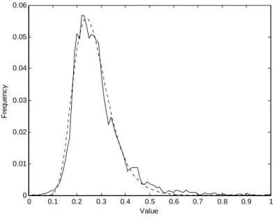
Figure 3: Distribution of Luck.
Luck realizations are normalized to lie between 0 and 1. The full line reflects the empirical distribution, whereas the dotted line is a fitted Frechét distribution. See the working version of the paper for estimation details.
0 0.1 0.2 0.3 0.4 0.5 0.6 0.7 0.8 0.9 1 0
0.01 0.02 0.03 0.04 0.05 0.06
Value
F
re
quenc
To estimate equation (11), we assume that the return function f takes the functional form in equation (9). We also assume that luck displays first order autocorrelation: εit =ρεi t, 1− +υit, where υit is an iid random variable with zero mean and finite variance. We allow for serial correlation because Getmansky et al (2004) argue that hedge fund returns are autocorrelated, attributing this to the illiquidity of their investment positions. Thus, equation (11) is a fixed effect unbalanced panel with serially correlated errors. We estimate (11) using the
methodology of Baltagi and Hu (1999).
We find that the distribution of talentμi (talent) matches well a Laplace distribution – see
Figure 2. The Laplace distribution has two parameters: a sample mean μ and a shape parameterσμ, and has the following probability distribution function (PDF):
( )
1. 2
i
i e
μ μ μ σ
μ
ζ μ σ
− −
= (18)
The distribution of εit (luck) matches well a Frechét distribution, which has a shape parameterσ and a persistence parameterρ. See Figure 3. Its PDF is f the form
(
)
( ) ( )1 1
1
1
| .
t t
t t
e
t t
F e
ε ρε
σ ε ρε
σ
ε ε σ
− +−
+
− − +
+ = (19)
We assume that the distribution of entrants’ initial luck is drawn from a Frechét distribution with mean equal to the ergodic mean of F and standard error σε.
In total, the model has 15 parameters – , , , , , , , , , ,A p x φ ψ μ ρ κ δ σ σ σ ωε, μ, , r and ce. Many of the parameter values can be determined using estimates from the related literature, and by estimating equation (11). We assume that a period equals one year. The calibrated parameter values are reported in Table 1.
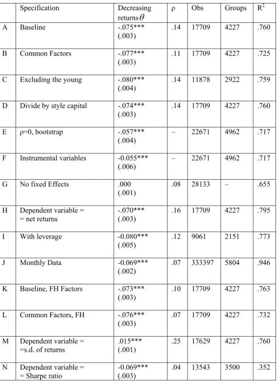
1. Decreasing returnsφ: In equation (11), φ−1 equals the coefficient of a fixed effect regression of hedge fund returns on size. The average value of this coefficient across different specifications is about -0.073. Thus, we set φ =0.927.
2. Spillover parameterψ : In principle we could estimate the spillover parameterψ using equation (11) by expanding the constant term D, given a measure of the capital under management at the competitors of a given hedge fund Qt-1 . In practice this is difficult because no hedge fund database is fully comprehensive (reporting is voluntary), and since hedge funds may compete with other types of fund managers. Using total capital at hedge funds in the same style in the CISDM database as a measure of Qt-1, we find that
0.035
outside this range. As we will see, qualitative results are similar. Notice that our estimate of 0.035
ψ = − lies within these bounds.
3. Common productivity A : we use this parameter to match the average fund size, which is $190 million in CISDM (2006) over the period 1994-2005.
4. Average “talent” μ is collinear with log A, we set it to zero without loss of generality. 5. Luck persistenceρ: In equation (11), this parameter is the AR(1) coefficient on the errors in a fixed effect regression of returns on size. We find that ρ = 0.14.
6. Variance of talentσμ: This parameter matches the standard deviation of returns in CISDM (2006).
7. Variance of luckσ : This parameter is set so that the ratioσ σε/ μ is as estimated. Across specifications we find that this ratio averages 0.82 across specifications, so that the variance of talent is slightly larger than the variance of luck.
8. Variance of entrant luckσε: We set the variance of entrant luck σε equal to σ, so that the environment faced by entrants is similar to that faced by incumbents. Since luck is not very persistent our results are robust to changes in the distribution of entrant luck.
9. Discount rate r : Integrating equation (14) over all funds in the industry, we have that average return in the industry equals:
( )
, 1(
, 1)
* , 1(
, 1)
** *
| log |
log 1 log .
i t
i t dF i t it d e dF i t it d
r
d d
ε
ε ε ε ξ ε ε ξ
φ
ξ ξ
+
+ + +
+ − +
∫ ∫
−∫ ∫
∫
∫
(20) We use an iterative procedure to calibrate r. We assume that the integral expressions equal zero, so this reduces to simply log 1
( )
+ −r logφ. Then we set the discount rate so that the average return on hedge funds equals 9.6% (as in the CISDM data), and compute the integrals once all the other parameters have been evaluated. Then given this sum, we compute the value of r that satisfies (19), and repeat. This implies a discount rate of 1.6%, which is about equal to the real value of 3-month LIBOR over the past 15 years.10. Average hazard rateδ: Getmansky (2004) argues that the average hazard rate of hedge funds is 7.1%. Liang and Park (2010) find that about a third of exits occur for reasons related to profitability, while the rest occur for other exogenous reasons. Thus, we set
= 7.1% 0.67 = 4.7%
e
δ × , and set probability s so that the overall exit rate equals 7.1%.
11. Initial cost of due diligence ce: We follow Brown et al (2008b) and set it to equal
12. Continuation costκ: We set the cost of continuing a fund equal to an estimate of the cost of ongoing due diligence to the investor. Brown et al (2008b) indicate that, at the Princeton University Investment Company this cost is about 7/40 of the initial due diligence cost.14 We take it as an indicator of the order of magnitude, suggesting that ongoing costs are considerably lower than startup costs. This implies that the fixed cost ce and the discounted expected cost of κaffect which funds enter, but that κhas very little impact on fund dynamics beyond entry.
13. Mass of entrants : Set so that the total industry capital in equilibrium equals $1.2 trn. 14. Leverage ratio x : CISDM defines the leverage ratio as the ratio of borrowed funds to capital. Recall that leverage ratios in CISDM are largely clustered around one (Figure 1). Malcolm et al (2009) and FSA (2009, 2010) find the same using different data sets. These numbers are based on self-reporting, and are imprecise – indeed, almost all the responses are integer-valued. This suggests there is some noise in the reported leverage – although the order of magnitude should be correct. Hence, we take 1 as the reported value of leverage. However, because hedge funds may also have “implicit” leverage via derivative positions, we use surveys to get an estimate of “effective” leverage. McGuire and Tsatsaronis (2008) find that “effective” leverage that includes synthetic borrowing (through derivatives) is about 10-20% higher than reported leverage. Hence we set x =1.1, and explore other values as well. 15. Cost of funds p : Calibrating the cost of funds p= + +
( )
1 k xc requires three inputs: the cost of leverage, the cost of equity, and the leverage ratio. We identify the borrowing cost c with 3-month LIBOR. This implies that c=0, recalling that the borrowing cost is paid up-front. We identify the cost of equity k with the equity risk premium,15 which is about 4%.Table 1: Parameters used in calibration
Parameters of the model economy are matched to data from different sources and to our econometric estimates. Details may be found in the text or in Appendix D.
A ψ φ ρ
μ
σ σ σε β κ ce e s x p
1.65 -.001, -.01
.927 .14 .175 .143 .143 .984 8750 50000 .047 .024 1.1 1.04
We take the opportunity to discuss the empirical relevance of the model. The model accounts for some well-known features of the hedge fund industry. For example, when the stochastic component of returns is not persistent, the optimal size at any given fund may be constant over time in a world of decreasing returns – see equations (6, 12). This suggests an explanation for the observation that hedge funds close to new investment after reaching a certain size. In addition, Berk and Green (2004) argue that the lack of evidence of persistent
14
See www.house.gov/apps/list/hearing/financialsvcs_dem/ht031307.shtml.
15
differences in returns across actively managed funds can coexist with large differences in manager talent because, in a world of decreasing returns, more talented managers optimally operate larger funds. We find a strong positive correlation between our measures of manager
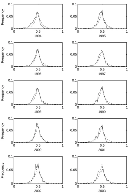
Figure 4: Manager fixed effects for entrants by year.
Fixed effects are estimated based on the full panel of hedge funds, and are normalized to lie between 0 and 1. The full line reflects the empirical distribution, whereas the dotted line is the fitted Laplace distribution in Figure 3, which matches the distribution of manager talent in the full sample. It has been rescaled to fit the
number of HFs in each panel, but the shape is preserved. Since at least two years of data are required to estimate each fund-specific fixed effect, and since return data were not available for all months in 2005, hedge funds born in 2004 and 2005 were not included.
0 0.5 1
0 0.05 0.1 1994 F requen c y
0 0.5 1
0 0.05 0.1
1995
0 0.5 1
0 0.05 0.1 1996 F reque nc y
0 0.5 1
0 0.05 0.1
1997
0 0.5 1
0 0.05 0.1 1998 F requ enc y
0 0.5 1
0 0.05 0.1
1999
0 0.5 1
0 0.05 0.1 2000 F req uenc y
0 0.5 1
0 0.05 0.1
2001
0 0.5 1
0 0.05 0.1 2002 F re quenc y
0 0.5 1
0 0.05 0.1
talent and fund size using the hedge fund data. Notably, the correlation between talent and size is positive, equal to 0.693 (s.e. 0.011), as predicted by equation (6). This finding is significant, as it provides evidence that the absence of persistent cross-fund differences in returns can be reconciled with the possibility of significant differences in manager talent if decreasing returns to scale lead more talented managers to optimally manage larger funds. A stylized fact of the asset management industry is that funds that outperform market
benchmarks tend to experience inflows of funds, a fact that has been viewed as a challenge to rational expectations and efficient market theory in light of the fact that persistent differences in performance across funds are difficult to detect – see Berk and Green (2004). In the presence of autocorrelated luck (Assumption 2), the model can account for such a finding because a positive realization of luck is correlated with positive realizations in the near future.
Finally, the model assumes a constant distribution of entrant talent across cohorts. Figure 4 plots the talent distributions for different cohorts in the data along with the Laplace
distribution that best fits the distribution of talent for all cohorts. While not identical in all years, the match is quite remarkable, underlining the usefulness of a model with the broad features of the Hopenhayn (1992) framework for analyzing hedge fund industry dynamics.
V. POLICY EXPERIMENTS
Having established the empirical relevance of the model, we now consider changes in different regulations, such as the cost of due diligence, the cost of leverage, and leverage limits, to see the impact on the number of the funds, total capital and profits in the model. We focus on regulations that can be interpreted in terms of model parameters, assuming other parameters remain constant. We discuss this assumption further at the end of the section.
A. The cost of due diligence
Suppose that the entry cost ce doubles from $50,000 to $100,000, which also doubles the continuation cost κ. See Table 2. This implies a decline in the returns (including due
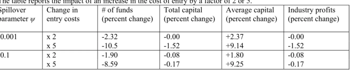
diligence costs) at the average fund of about 0.73 basis points.16 The number of funds drops by about 2 percent. However, industry assets under management are almost unchanged. This is because the funds that no longer exist in the stationary equilibrium with new parameters are all very small. Industry profits are unchanged, since the equilibrium rate of return
depends on φ (which is constant) and industry capital are negligibly affected. As a result, the average hedge fund capital under management rises also by about 2 percent.
Suppose that the entry cost is increased by a factor of five (to $250,000). Then the number of funds declines by about 10 percent, which leads to a 1.5 percent drop in the industry capital
16
(and total industry profits). Thus, a large change in the cost of due diligence (or other fixed costs of entry or continuation) can have a large effect on the number of funds, but the impact on the size of the industry is an order of magnitude lower, since the affected funds are small. It is perhaps not surprising that changes in the cost of due diligence have a small effect on the hedge fund industry, since both ce and κ are too small relative to the returns at most of the hedge funds. To get a sense of this, the average expected cost of due diligence over the lifetime of a hedge fund is about $173,000, whereas the expected return to the average entrant is about $166 million.
Table 2: Experiments – raising the cost of entry
The table reports the impact of an increase in the cost of entry by a factor of 2 or 5. Spillover
parameterψ
Change in entry costs
# of funds (percent change)
Total capital (percent change)
Average capital (percent change)
Industry profits (percent change)
-0.001 x 2 -2.32 -0.00 +2.37 -0.00
x 5 -10.5 -1.52 +9.14 -1.52
-0.1 x 2 -1.90 -0.08 +1.80 -0.08
x 5 -8.59 -0.17 +9.25 -0.17
It should be noted that the impact of a higher cost of due diligence is smaller when the spillover parameter ψ (the sensitivity of the hedge fund returns to the total capital of all funds) is large. As ψ → 0, all adjustment to stricter regulation must be carried out by each individual hedge fund. However, when there are significant cross-fund spillovers (ψ is large), the fact that other funds optimally shrink goes some way towards offsetting the profit loss from the higher due diligence cost at any given hedge fund. Still, the impact of
regulation is qualitatively similar for both values of ψ we consider. Thus, whatever the hypothetical benefits of increasing the creation and continuation costs of hedge funds might be, the impact on the industry as a whole of higher costs is not likely to be significant.
B. The cost of leverage
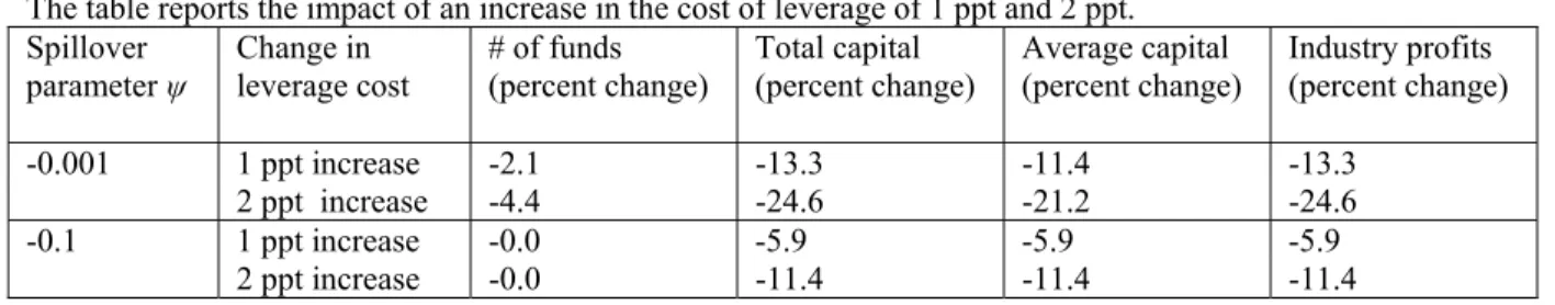
How would an increase in the cost of leverage impact equilibrium outcome in the industry? Suppose that the cost of leverage rises by 1 percentage point (comparable to a spike in 3-month LIBOR in late 2008, which was of magnitude 1.2 percent). An increase in the cost of leverage by 1 percentage point can have a large impact on industry capital (and hence on total profits), especially when the spillover parameter is small, but only a modest impact on the number of funds. See Table 3.
Increasing the cost of leverage has larger impact on industry capital under management for smaller values of spillover parameterψ . The reason is that, holding industry capital
tend to increase optimal capital at any given fund. This offsetting effect is only significant when the spillover parameter ψ is large (i.e., whenψ = −0.1, the decrease in equilibrium capital is less than half of the decrease when ψ = −0.001).
Table 3: Experiments – raising the cost of leverage
The table reports the impact of an increase in the cost of leverage of 1 ppt and 2 ppt. Spillover
parameterψ
Change in leverage cost
# of funds (percent change)
Total capital (percent change)
Average capital (percent change)
Industry profits (percent change)
-0.001 1 ppt increase -2.1 -13.3 -11.4 -13.3
2 ppt increase -4.4 -24.6 -21.2 -24.6
-0.1 1 ppt increase -0.0 -5.9 -5.9 -5.9
2 ppt increase -0.0 -11.4 -11.4 -11.4
By contrast, increasing the cost of leverage has a modest impact on the number of funds when ψ = −0.001 – and a negligible impact whenψ = −0.1. The reason is that even a large decrease in equilibrium capital (and hence in total profits) at a given type of fund is unlikely to drive its value below the cost of entry: the marginal hedge fund (whose value on entry equals the entry cost) is far in the left tail, and the profits of most funds are orders of magnitude larger.
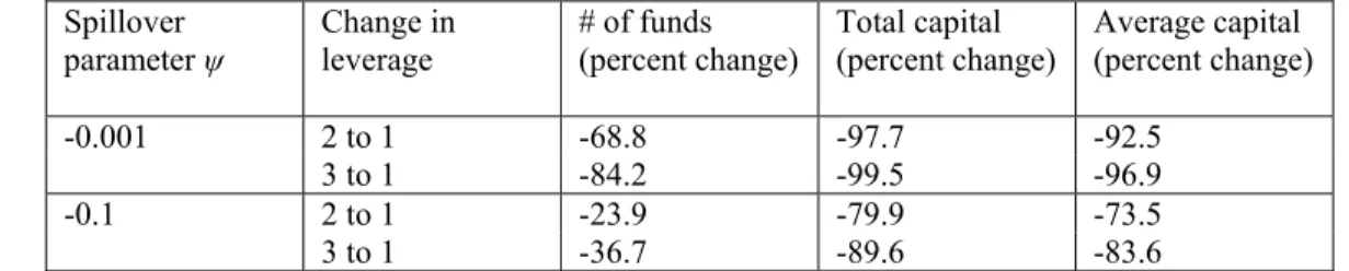
C. Leverage limits
Next, consider the imposition of leverage limits, below the current industry best practice. There are two channels in the model through which leverage caps might affect the hedge fund industry. The first is by reducing the “productivity” of capital, since under a lower leverage ratio a dollar of capital allows to establish a smaller investment position. Second, leverage caps reduce the effective cost of capital p (since the cost of funding a dollar of capital is p≡ + +
( )
1 k xc.) If the cost of leverage is lower than the cost of capital (as in practice), this second channel is likely to be small. Indeed, since the calibrated value of the cost of leverage c=0, the second channel is absent from our baseline experiments. However, we later show that introducing this channel does not change the results.Suppose that the current industry best practice leverage ratio is 1.1 What would be the impact from lowering it to 1 or to 0.9?17 We find that while industry capital declines very sharply, the decline in the number of funds is fairly modest. See Table 4.
When leverage ratio is reduced from 1.1. to 1, industry capital declines by 21-46 percent, depending on the value of the spillover parameter ψ . This is because lower leverage limit leads to a dramatic reduction in the “productivity” of capital, which lowers the optimal capital of a hedge fund. Again, there is an offsetting effect from other funds reducing their leverage as well. However, when the spillover parameterψ = −0.001, this effect is negligible.
17
The equilibrium rate of return is not significantly affected by changes in leverage ratios. Thus, the impact on the total profits of the industry is the same as the impact on its size.
Table 4: Experiments – lowering the leverage ratio
The table reports the impact of a decrease in the leverage ratio from 1.1 to 1 and to 0.9 Spillover
parameterψ
Change in leverage
# of funds (percent change)
Total capital (percent change)
Average capital (percent change)
Industry profits (percent change)
-0.001 1.1 to 1 -6.8 -45.7 -41.7 -45.7
1.1 to 0.9 -18.9 -71.4 -64.8 -71.4
-0.1 1.1 to 1 -1.9 -20.8 -19.3 -20.8
1.1 to 0.9 -4.0 -38.0 -35.5 -38.0
When leverage ratio is reduced from 1.1. to 1, the number of active hedge funds declines by 2-7 percent, depending on the value of the spillover parameter ψ . Why is the number of hedge funds much less sensitive to the imposition of leverage cap than the industry capital? Consider that the productivity of a firm with talent two standard deviations above the mean is almost double the productivity of a firm two standard deviations below the mean. Since decreasing returns due to the parameter φ are not steep, a small difference in productivity translates into a significant difference in profits: the expected lifetime profits of a firm with talent two standard deviations above the mean is about $1.37 billion, whereas those of a firm two standard deviations below the mean are about $1.32 million. As a result, even a very large drop in profits across the hedge fund industry has little impact on the number of funds, because the range of the productivity distribution whose expected lifetime profits are driven below ce by the change is small.
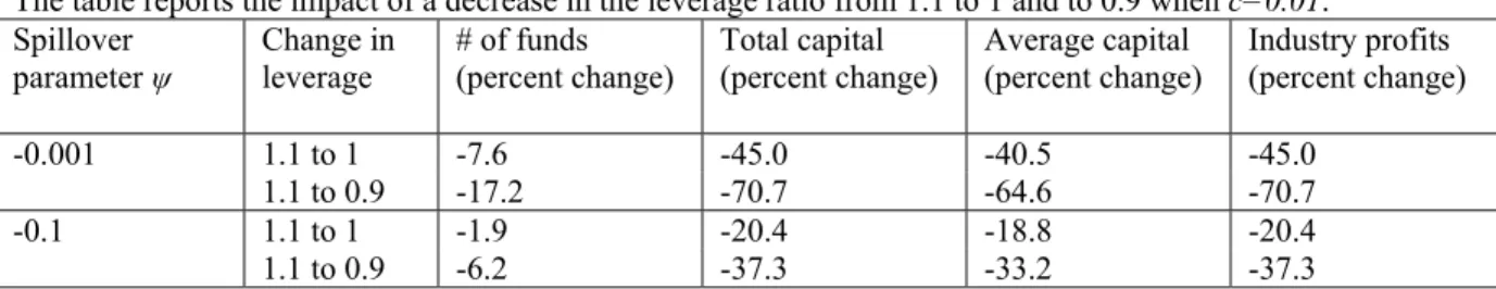
Table 5: Experiments – lowering the leverage ratio when c=0.01
The table reports the impact of a decrease in the leverage ratio from 1.1 to 1 and to 0.9 when c=0.01. Spillover
parameterψ
Change in leverage
# of funds (percent change)
Total capital (percent change)
Average capital (percent change)
Industry profits (percent change)
-0.001 1.1 to 1 -7.6 -45.0 -40.5 -45.0
1.1 to 0.9 -17.2 -70.7 -64.6 -70.7
-0.1 1.1 to 1 -1.9 -20.4 -18.8 -20.4
1.1 to 0.9 -6.2 -37.3 -33.2 -37.3
Table 5 repeats these experiments assuming that c=0.01. In this way, the “cost of funding” channel is present also. Notice that results are almost identical. The reason is that, for this value of c, a reduction in leverage from 1.1 to 1 lowers the cost of funding p from 1.051 to 1.05, a 0.1 percent change. If c=0.02, then such a change in leverage would still only lower the cost of funding by 0.2 percent. Thus, only an unrealistically high cost of leverage would allow the cost-of-funding channel to significantly impact results.
D. Size-contingent leverage limits
initial leverage ratio, and let xnew<x be a newly–imposed leverage limit. Suppose that the regulator chooses to impose the new leverage ratio only on hedge funds whose capital exceeds a certain size threshold ς. For example, ς could be selected so as only to affect the largest 25 percent (or the largest 1 percent) of hedge funds. Then, leverage limit x applies if
, 1
i t
q − ≤ς and xnew applies if qi t, 1− >ς .
Table 6: Experiments – leverage caps with size allowances
The table reports the impact of a decrease in the leverage ratio from 1.1 to 1. Assumes that ψ= -0.001. Size Allowances below which leverage ratios do not apply Statistic
0 1.2e+7 1e+8 6.9e+9 1e+10 1.82e+10
% of funds originally below 0 73.1 89.7 99.3 99.5 99.9
% of capital at funds originally below 0 1.1 4.2 50.1 62.0 87.9
% of funds at the limit 0 5.9 2.5 0.45 0.38 0.11
% of capital at funds at limit 0 0.7 2.4 20.4 23.1 10.8
% of funds below the limit 0 74.6 90.1 99.3 99.5 99.9
% of capital at funds below 0 1.9 7.2 61.4 70.4 89.2
% change in number of funds -6.8 0 0 0 0 0
% change in total capital -45.7 -45.1 -43.5 -18.7 -12.2 -1.3 % change in average capital -41.7 -45.1 -43.5 -18.7 -12.2 -1.3
% change in ex post returns -0.51 -0.63 -0.10 -0.09 -0.04 -0.00
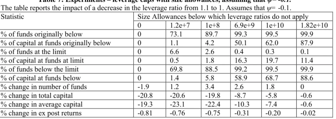
Table 7: Experiments – leverage caps with size allowances, assuming that ψ= -0.1.
The table reports the impact of a decrease in the leverage ratio from 1.1 to 1. Assumes that ψ= -0.1. Size Allowances below which leverage ratios do not apply Statistic
0 1.2e+7 1e+8 6.9e+9 1e+10 1.82e+10
% of funds originally below 0 73.1 89.7 99.3 99.5 99.9
% of capital at funds originally below 0 1.1 4.2 50.1 62.0 87.9
% of funds at the limit 0 6.6 2.6 0.4 0.3 0.1
% of capital at funds at limit 0 0.5 1.8 16.3 19.7 11.4
% of funds below the limit 0 69.8 88.5 99.2 99.5 99.9
% of capital at funds below 0 1.4 5.8 58.9 68.7 88.6
% change in number of funds -1.9 1.2 3.4 2.6 1.8 0
% change in total capital -20.8 -20.6 -19.8 -8.7 -5.8 -0.6
% change in average capital -19.3 -23.1 -22.4 -10.3 -7.4 -0.6
% change in ex post returns -0.81 -0.76 -0.75 -0.31 -0.20 -0.02
An analytical characterization of problem (8) with size-contingent leverage caps is omitted. However, it is straightforward to show that the fund’s optimal strategy is to choose between three candidate capital values: one assuming leverage ratio x, another assuming leverage ratio xnew , and the size limit itself ς. Since xnew<x implies that x is more profitable, the solution for the old leverage ratio xwill be adopted unless this involves the hedge fund size exceeding the limit ς. If so, the solution will be the optimum assuming that leverage is xnew – unless this turns out to be lower than the optimum under x. If so, then the optimal size is ς itself. See, Veracierto (2008) for a proof of a similar model in the context of evaluating the equilibrium impact of firing costs on employment.
There is no guidance in the literature as to what constitutes a likely size threshold ς, so we explore a variety of values. Tables 6-7 reports the results of the experiments with leverage caps for different size thresholds. While a leverage ratio without a size threshold