Discussion Paper Series A No.627
Japanese Fiscal Policy under the Zero Lower Bound of Nominal Interest Rates:
Time-Varying Parameters Vector Autoregression
Hiroshi Morita
(Japan Society for the Promotion of Science, Research Fellowship for Young Scientists)
July, 2015
Institute of Economic Research Hitotsubashi University Kunitachi, Tokyo, 186-8603 Japan
Japanese Fiscal Policy under the Zero Lower Bound of Nominal
Interest Rates:
Time-Varying Parameters Vector Autoregression
✩Hiroshi Morita
Japan Society for the Promotion of Science, Research Fellowship for Young Scientists Institute of Economic Research, Hitotsubashi University
Naka 2-1, Kunitachi-City, Tokyo 186-8603, Japan
Abstract
This study investigates whether the effects of fiscal policy are enhanced during ZLB periods. We present a new strategy for identifying unconventional monetary policy shocks in the framework of a time-varying parameters vector autoregressive model. The main findings are as follows. First, during ZLB periods, the volatility of short-term interest rates is quite small, while that of the monetary base is large. Second, fiscal policy shocks have significant positive time-varying effects on GDP after adoption of unconventional monetary policy. Third, the effects of fiscal policy shocks increase during a ZLB period.
JEL classification: E62, E52, C11, C32
Keywords: TVP-VAR model, zero lower bound, sign restriction, fiscal policy
✩We would like to appreciate Etsuro Shioji, Toshiaki Watanabe, Naohito Abe, Minoru Tachinaba, Hi- rokuni Iiboshi and seminar participants at the 2014 spring meeting of Japan Economic Association, Western Economic Association International 11th International Conference, and The 11th International Symposium on Econometric Theory and Applications (SETA2015), for helpful comments and suggestions. I would like to express gratitude to the research fellowships of the Japan Society for the Promotion of Science (JSPS) for Young Scientists for the grant that made it possible to complete this study. Of course, all errors are my own.
Email address: hiroshi.morita1013@gmail.com(Hiroshi Morita)
1. Introduction
After recent financial crises, such as the Lehman Brothers shock and the European debt crisis, the authorities of major industrialized economies have been implementing aggressive fiscal policies and monetary easing simultaneously. In particular, the central banks of those economies have conducted quantitative easing (QE) at the zero lower bound (ZLB) of nominal interest rates as part of unconventional monetary policy. There is active discussion and growing literature on the effectiveness of those economic policies. The aim of this study is to evaluate the effects of these fiscal and monetary policies in Japan, using the time-varying parameters vector autoregressive (TVP-VAR) model with stochastic volatility developed by Primiceri (2005). As pointed out in several previous studies, Japan is “a front-runner of unconventional monetary policy (Kimura and Nakajima, 2013)” and has experienced a zero interest rate for a sufficiently long time (Hayashi and Koeda, 2013). In addition, a large number of fiscal stimulus packages have been implemented in Japan since the collapse of the bubble economy in the early 1990s (Fukuda and Yamada, 2011). Therefore, the Japanese economy is an appropriate and interesting subject for our research. In addition, the TVP- VAR model enables us to estimate the time-varying effects of those economic polices without dividing the sample period.
This study contributes to the existing literature as follows. First, we present a new method for identifying monetary policy at the ZLB of the nominal interest rate. There are several VAR analyses about Japanese monetary policy after QE.1 For example, Honda et al. (2007) identify monetary policy shock by regarding current account balances as a monetary policy instrument, and report that QE increases output through the stock price channel. However, their sample period only covers 2001 to 2006, when the Bank of Japan (BOJ) conducted QE policy. On the other hand, Fujiwara (2006) and Inoue and Okimoto (2008) estimate a Markov-switching VAR model using both conventional and unconventional monetary policy periods. Both these studies conclude that regime change occurred in the late 1990s, and that the effectiveness of monetary policy seems to decrease after the structural change. More recently, Hayashi and Koeda (2013) estimate a two-regime structural VAR model and incorporate an exit condition from zero interest rate policy, in which the monetary
1Miyao (2002) and Shioji (2000) analyze Japanese monetary policy before QE.
policy regime changes when a certain condition about the inflation rate is satisfied. In addition, they find expansionary effects of monetary policy on inflation and output. Similar to studies using the TVP-VAR model, Franta (2011), Kimura and Nakajima (2013), Nakajima (2011a), and Nakajima et al. (2011) also estimate the time-varying effects of monetary policy in Japan.
Although each previous study provides sufficient attention to the identification of mone- tary policy, the characterization of monetary policy under the ZLB of nominal interest rates can be improved. With the exception of Franta (2011), monetary policy shocks are commonly identified as those that lower interest rates (e.g., Fujiwara, 2006; Inoue and Okimoto, 2008; Nakajima, 2011a). In addition, often interest rate and monetary base shocks are identified separately (e.g., Hayashi and Koeda, 2013; Kimura and Nakajima, 2013). It seems to be inappropriate to identify monetary policy shocks in this manner because there is no room to lower interest rates in ZLB periods. In addition, rate cuts are usually performed through the supply of the monetary base to the market, and thus, monetary policy shocks should be characterized by both monetary variables. The next point is related to the dynamics of short-term interest rates in the ZLB. As noted in Nakajima (2011a), the effects of structural shocks are unlikely to work through the interest rate channel at the ZLB periods because the policy rate falls to zero. Nevertheless, previous studies, with the exception of Nakajima (2011a) and Kimura and Nakajima (2013), allow short-term interest rates to vary in response to structural shocks even in the ZLB. To resolve these difficulties, we incorporate zero re- strictions into the short-term interest rate equation based on Nakajima (2011a), and identify monetary policy shocks as a combination of interest rates and the monetary base, following Franta (2011).
More precisely, by using sign restrictions, monetary policy shocks are characterized as those that lower short-term interest rates and raise the monetary base, and a non-negativity constraint is imposed on short-term interest rates. Intuitively, this constraint eliminates the possibility that interest rates fall more than the observed rates in response to monetary policy shocks. On the other hand, zero restrictions on the coefficient and contemporaneous relations in the interest rate equation allow interest rates to be fixed during the ZLB periods. By combining the abovementioned two methodologies, we are able to identify the effects of monetary policy under the ZLB of nominal interest rates.
In addition to presenting the new identification for monetary policy, this study contributes to the literature by analyzing the effects of fiscal policy. This is motivated by the theoretical prediction presented by Braun and Waki (2006), Christiano et al. (2011), and Eggertsson (2010), who theoretically show that the effects of fiscal policy are enhanced at the ZLB. We investigate whether this theoretical prediction can be observed empirically. Furthermore, we rely on the claim of Rossi and Zubairy (2011), who show that unbiased estimates of the effects of fiscal and monetary policy shocks cannot be obtained unless we identify both fiscal and monetary policies simultaneously. In the spirit of Rossi and Zubairy (2011), Gerba and Hauzenberger (2014) attempt to estimate the fiscal and monetary interactions in the US economy by using a TVP-VAR model.2 However, Gerba and Hauzenberger (2014) do not specifically identify monetary policy under the ZLB. To my knowledge, there are no studies analyzing time-varying effects of both fiscal and monetary policies taking the ZLB of nominal interest rates into account.
The main results obtained in this study are summarized as follows. First, in ZLB periods, the volatility of short-term interest rates is estimated to be fairly small and the volatility of the monetary base is quite large. Second, the results of impulse response function (IRF) analysis show that the effects of fiscal policy, which is characterized as a surprise increase in government spending, have changed over time. In particular, the response of GDP to fiscal policy shocks indicates a sign switch after the mid-1990s. Third, we are able to confirm that the effects of fiscal policies are enhanced during the ZLB period, as is predicted theoretically by Christiano et al. (2011) and Eggertsson (2010). Moreover, this increase in the effects of fiscal policy at the ZLB periods is caused through the consumption channel.
After obtaining our main results, robustness checks are performed. First, the ZLB periods are redefined by taking the interest rate payment on the bank reserve into consideration.3 In addition, a model is estimated in which GDP is replaced with private consumption or private investment.
2In addition, Kirchner et al. (2010) and Pereira and Lopes (2014) estimate the TVP-VAR model in the US and Euro area, respectively. However, they focus only on the effects of fiscal policy shock.
3Since November 2008, the BOJ has paid an interest rate of 0.1% on the bank reserve and then, the net interest rate, calculated by subtracting the rate paid on the reserve from the call rate, falls below 50 basis points.
The rest of this paper is structured as follows. In Section 2, we explain the empirical framework adopted in this study. Specifically, we describe the TVP-VAR model with sign restrictions, the identification strategy, and the Bayesian technique. Section 3 presents the data and the specifications employed. Section 4 shows the estimated results of the volatility, the IRFs, and the fiscal multiplier. Section 5 performs robustness checks. Section 6 presents our conclusions.
2. Estimation methodology
2.1. Time-varying parameters VAR model
As stated in Section 1, this study employs the TVP-VAR model with stochastic volatility, developed by Primiceri (2005). For a k-dimensional vector of endogenous variables, yt = (y1t, · · · , ykt), the structural-form TVP-VAR model is formulated as
Atyt= B0t+ B1tyt−1+ · · · + Bstyt−s+ ut, t = s + 1, · · · , T, (1)
ut∼ N (0, ΣtΣ′t), (2)
where Bit(i = 0, · · · , s) are k × k matrices of time-varying coefficients and At are k × k matrices of time-varying coefficients specifying the contemporaneous relations among the endogenous variables. Moreover, At is assumed to be a lower-triangular matrix given by
At=
1 0 · · · 0
a21t 1 · · · ...
· · · . .. . .. ... ak1t · · · ak,k−1,t 1
. (3)
The disturbance ut denotes the vector of structural shocks, which is distributed according to a k-dimensional normal distribution with mean 0 and time-varying covariance matrix ΣtΣ′t, where
Σt=
σ1t 0 · · · 0 0 . .. ... ... ... ... ... 0 0 . .. 0 σkt
. (4)
By multiplying both sides of Eq.(1) by A−1t , the reduced-form VAR model that we estimate is given as
yt= C0t+ C1tyt−1+ · · · + Cstyt−s + A−1t Σtεt, (5)
εt ∼ N (0, Ik), (6)
where Cit = A−1t Bit(i = 0, · · · , s), and εt is a vector of structural shocks that are normalized to be of variance 1. Defining βt = [vec(C0t)′, · · · , vec(Cst)′]′ and Xt = Ik⊗ (1, yt−1′ , · · · , yt−s′ ), where ⊗ denotes the Kronecker product, Eq.(5) can be transformed to
yt= Xtβt+ A−1t Σtεt. (7) Subsequently, we set the process for the time-varying parameters. Let at be a stacked vector of the lower triangular elements in At and ht = (h1t, · · · , hkt)′ with ht = ln(σit2). As in Primiceri (2005), we assume that the time-varying parameters evolve according to a random walk process, as follows:
βt+1 = βt+ uβt, αt+1 = αt+ uαt, ht+1 = ht+ uht,
for t = s + 1, · · · , T , where βs+1 ∼ N (µβ0, Σβ0), αs+1 ∼ N (µα0, Σα0) and hs+1 ∼ N (µh0, Σh0). Moreover, the model innovations are assumed to be uncorrelated among the parameters βt, αt, and ht, as follows:
εt
uβt
uαt
uht
∼ N
0,
Ik 0 0 0
0 Σβ 0 0
0 0 Σα 0
0 0 0 Σh
,
where the variance-covariance structure for the innovations of the time-varying parameters (Σβ, Σα, Σh) is assumed to be a diagonal matrix.
2.2. Identification
By extending the TVP-VAR model, we attempt to reveal the effects of fiscal policy under the ZLB of nominal interest rates as well as the effects of monetary policy. For this purpose, our benchmark VAR system consists of the short-term interest rate, monetary base, government spending, and GDP in this order.4 Furthermore, to characterize the transmission mechanism of monetary policy under the ZLB, two kinds of restrictions are added to the VAR coefficients and the contemporaneous relationship among the variables.
The first restriction is related to the VAR coefficients of the interest rate equation. As stated in Nakajima (2011a), the effect of monetary policy does not seem to prevail through the interest rate channel at the ZLB. Moreover, it seems that hardly any shocks are able to affect interest rates because the monetary authority fixes the rates to almost zero. In other words, the variations of the interest rates to the shocks vanish once the rates hit the ZLB. To replicate this dynamic property of interest rates, Nakajima (2011a) proposes the TVP-VAR-ZLB model in which the coefficients of the interest rate equation are assumed to stick to zero during ZLB periods.5 The present study also adopts the restriction of the TVP-VAR-ZLB model to characterize the dynamics of monetary policy during the ZLB by following Nakajima (2011a).
The second restriction is associated with the contemporaneous relationship among endoge- nous variables, that is, the identification of structural shocks. A shortcoming of Nakajima (2011a) exists in the identification scheme, in which an innovation in interest rates is re- garded as a monetary policy shock. As a result, monetary policy shocks have no effects on other variables during ZLB periods. Although there are many studies that recognize short- term interest rates as policy targets of monetary authorities, as represented by Christiano et al. (1999), several studies (e.g., Mountford and Uhlig, 2009) characterize monetary policy shocks by combining interest rates and the monetary base. In Japan, especially, there are many studies in which the monetary base or bank reserve is regarded as a target of mon- etary policy since the BOJ adopted QE policy (e.g., Hayashi and Koeda, 2013; Honda et
4Except for the short-term interest rate, each variable is included in the form of the log first-difference. Government spending is defined as the sum of government consumption and public investment. A detailed description of the data is provided later.
5In the next section, we describe how to impose this assumption on the estimated equation.
al., 2007; Kimura and Nakajima, 2013). In line with this strand of studies, we characterize monetary policy shocks by using the short-term interest rates and the monetary base. More precisely, we distill shocks that increase the monetary base but lower short-term interest rates as monetary policy shocks by using the sign restriction developed by Uhlig (2005).
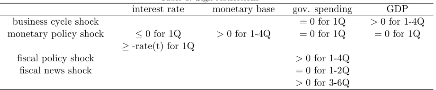
In addition to monetary policy shocks, this study identifies business cycle shocks and two types of fiscal policy shocks: unanticipated and anticipated. In the spirit of Ramey (2011), who points out the importance of fiscal foresight, we also focus on the effects of anticipated fiscal policy shocks (hereafter, fiscal news shocks) as well as unanticipated fiscal policy shocks (hereafter, fiscal policy shocks). The sign restrictions adopted in this study are summarized in Table 1.
[Table 1 about here.]
These restrictions essentially follow the previous studies. First, fiscal policy shocks are identified under the standard assumption that government spending is the most exogenous variable, and thus, is affected only by this type of shock at the impact period. This assump- tion is based on the fact that fiscal policy cannot react immediately to changes in the state of the economy owing to the decision lag. This fact has been accounted for by most previ- ous studies (e.g., Blanchard and Perotti, 2002; Gal´ı et al., 2007). Furthermore, government spending is assumed to be positive for the first four periods in response to fiscal policy shocks. Second, the restriction for identifying fiscal news shocks is based on Mountford and Uhlig (2009). Supposing a situation in which government spending does not change immediately after fiscal news is announced, a zero restriction is associated with the responses of govern- ment spending for the first two periods. Thereafter, it is assumed that government spending increases from the third to the sixth periods. Third, as stated earlier in this subsection, monetary policy shocks are defined as those that lower short-term interest rates and increase the monetary base. This assumption is widely accepted in previous studies that examine the effects of monetary policy by using sign restrictions (e.g., Franta, 2011; Mountford and Uhlig, 2009; Uhlig, 2005). In addition to these restrictions, we assume that monetary policy has no effects on GDP at the impact period, as in Christiano et al. (1999). Moreover, the non-negativity constraints are incorporated to rule out the possibility that interest rates fall more than the observed rates in response to monetary policy shocks, as adopted in Franta
(2011). Finally, business cycle shocks are defined simply as those that increase GDP for the first four periods, following Mountford and Uhlig (2009).
2.3. Estimation process
As widely employed in the literature, the TVP-VAR model is estimated via Bayesian ap- proach using the Markov-chain Monte Carlo (MCMC) method in this study. In the Bayesian estimation, the joint posterior distribution of parameters is calculated from the prior distribu- tion and the observed data. The MCMC algorithm enables us to sample the parameters from the full conditional posterior distribution even if the posterior distribution cannot be written down analytically. Since the TVP-VAR model comprises many parameters, and thus, the posterior is too complicated to calculate, the MCMC method is suitable for the estimation. This subsection briefly explains the process of estimation.6
Let us define β = {βt}Tt=s+1, α = {αt}Tt=s+1, h = {ht}Tt=s+1, ω = (Σβ, Σα, Σh), and y = {yt}Tt=s+1. Given the data y and the prior density function π(Θ), where Θ = β, α, h, ω, the samples from the posterior distribution π(Θ | y) are obtained as follows:
1. Set initial value of β(0), α(0), h(0), ω(0), and set j = 1. 2. Draw β(j+1) from π(β | α(j), h(j), Σ(j)β , y).
3. Draw Σ(j+1)β from π(Σβ | β(j+1)).
4. Draw α(j+1) from π(α | β(j+1), h(j), Σ(j)α , y). 5. Draw Σ(j+1)α from π(Σα | α(j+1)).
6. Draw h(j+1) from π(h | β(j+1), α(j+1), Σ(j)h , y). 7. Draw Σ(j+1)h from π(Σh | h(j+1)).
8. Identify structural shocks based on β(j+1), αj+1 and h(j+1) using sign restrictions. 9. Return to step.2 until N iterations have been completed.
For the above, N is set at 60, 000, but only every 10th draw is saved in order to alleviate the autocorrelation among each draw. In addition, only draws in which the roots of the VAR coefficients are inside the unit circle throughout the sample period are selected in order to
6A detailed explanation of the estimation process of the TVP-VAR model is described in Nakajima (2011a) and Nakajima (2011b).
ensure the stationarity of the VAR system. Furthermore, the first N0 = 10, 000 samples are discarded as burn-in. As a result, the inference is implemented based on a sample of 5, 000.
For sampling β and α, we employ a simulation smoother (De Jong and Shephard, 1995; Durbin and Koopman, 2002) because our model forms a state space formulation by regarding the time-varying parameters as latent variables. In particular, the sampling β during the ZLB period is performed based on Nakajima (2011a). As stated in Subsection 2.2, the coefficients of the interest rate equation are restricted to zero in the ZLB period. To produce this situation, we takes the following means for sampling β in step 2. First, we replace the elements of Σβ that correspond to the coefficients of the interest rate equation to zero when interest rates hit the lower bound. By doing so, the innovations uβt associated with the coefficients of the interest rate equation disappear in the ZLB period, and thus, the corresponding elements of βt stick to the most recent value before the ZLB period. Thereafter, we substitute the values of the coefficients associated with the interest rate equation in the ZLB period with zero. With respect to sampling the stochastic volatility h, we use the multi-move sampler of Watanabe and Omori (2004), whose algorithm generates samples from the exact conditional posterior density of h.
The identification of the structural shocks in step 8 is explained in detail as follows. For the endogenous variables in the VAR model, we identify four types of structural shocks: business cycle, monetary policy, fiscal policy, and fiscal news. We distill these shocks by using the sign restrictions presented in Mountford and Uhlig (2009). Given the random samples of β, α, and h in each iteration, we first calculate the impulse response vector a(1)t associated with fiscal news shock by using q(1)t , where qt(1) satisfies qt(1)′q(1)t = 1, and the zero restriction on government spending for the first two periods,
0 = R1tqt(1), (8)
where Rt1 is a 2 × k matrix, denoted as
R1t =
rj1t(1) · · · rjkt(1) rj1t(2) · · · rjkt(2)
. (9)
Here, ritj(p) is the response of the j-th variable (government spending here) to the i-th column of A−1t Σt at period t in horizon p. By this restriction, the response of government spending
for the first two periods is set to be zero. Using this q(1)t , the impulse response vector a(1)t is obtained by
a(1)t = A−1t Σtq(1)t . (10) Subsequently, the impulse response vector to monetary policy shocks a(2)t is calculated by using q(2)t , where the restrictions qt(2)′qt(2) = 1, q(2)t ′qt(1) = 0 are imposed on q(2)t to satisfy orthonormality. Furthermore, in order to achieve a situation in which monetary policy has no contemporaneous effects on GDP and government spending, the additional restriction is imposed on qt(2). This restriction can be written as
0 = R2tqt(2), (11)
where Rt2 is 2 × k matrix of the form
R2t =
rj1t(1) · · · rjkt(1) rl1t(1) · · · rlkt(1)
. (12)
Similar to the element of Rt1, rlit(p) is the response of the l-th variable (GDP here) to the i-th column of A−1t Σt at period t. Given q(2)t , a(2)t can be derived as in Eq.(10).
Likewise, business cycle shocks are identified using q(3)t , which satisfies orthonormality [qt(1), qt(2), q(3)t ]′× [q(1)t , qt(2), qt(3)] = [0, 0, 1]′ and the exogenous condition of government spend- ing,
0 = R3tqt(3), (13)
where Rt3 is a 1 × k matrix, denoted as
R3t =[rj1t(1) · · · rjkt(1)
]. (14)
Finally, the impulse response vector to fiscal policy shocks a(4)t is derived by using qt(4), which satisfies [qt(1), qt(2), qt(3), q(4)t ]′× [qt(1), qt(2), q(3)t , q(4)t ] = [0, 0, 0, 1]′.
In each period of each iteration, the abovementioned procedure is repeated until the impulse responses satisfy the sign restrictions, or the draws of qt reach 100. If the sign restrictions are satisfied for the entire sample period, the new contemporaneous relation calculated by {qt}Tt=s+1 is saved as a valid draw. If a valid draw is not provided in 100 draws, we return to step 2 without preserving any results.
3. Data and specification
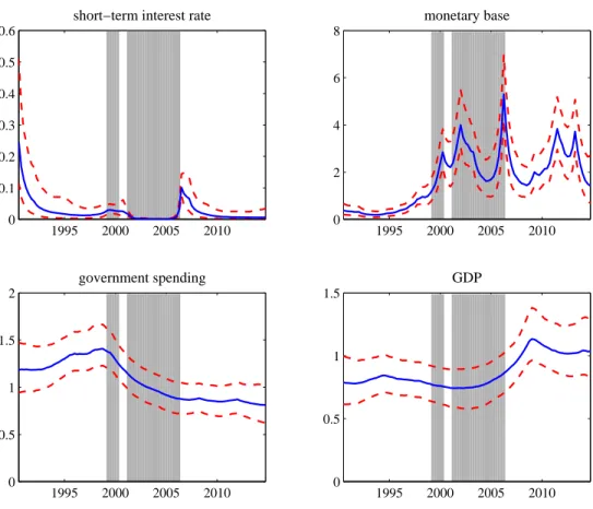
We employ the quarterly series of short-term interest rates, monetary base, government spending, and GDP covering the period from 1980Q1 to 2014Q4. The sample period is from 1990Q1 to 2014Q4, and the pre-sample period, from 1980Q1 to 1989Q4, is used to calibrate the prior distribution for the initial state of the time-varying parameters. The short-term interest rates are the call rates that correspond to the policy rate in Japan. Following Miyao (2002), we combine the uncollateralized overnight rate after July 1985 and the collateralized overnight rate until June 1985 by adding the mean difference between the two series to the collateralized rate until June 1985. Thereafter, we construct the quarterly series of short- term interest rates by taking the average for 3 months. Government spending is defined as the sum of government consumption and public investment. The series, except for the short- term interest rates, are seasonally adjusted per capita. The data for government spending and GDP are obtained from the System of National Accounts (SNA) database in Japan, and released by the Cabinet Office of the Government of Japan. The monetary data (i.e., the short-term interest rates and the monetary base) are obtained from the Bank of Japan. In addition, the total population data that are used to convert the variables to per capita value are collected from the Japanese Population Census (Ministry of Internal Affairs and Communication).
The estimated VAR system includes the log first difference of government spending, mone- tary base, GDP, and the levels of the short-term interest rates as well as a constant term. The number of lags is set to be two, which is often used in the literature because the TVP-VAR model comprises too many parameters if a high-order lag is chosen.
With respect to the ZLB period, this study follows the definition of Nakajima (2011a). Accordingly, we define the periods in which the short-term interest rates fell below 50 basis points as the ZLB periods. In Figure 1, which plots the data in the VAR model, the shaded areas refer to the ZLB periods and these correspond to the periods from 1999Q2 to 2000Q2 and from 2001Q2 to 2006Q2.
The prior distributions for the i-th element of Σj, j = β, α, h, denoted by ωji2, j = β, α, h, are assumed to be
ωβi2 ∼ IG(10, 0.01), ω2αi ∼ IG(2, 0.01), ω2hi∼ IG(2, 0.01). (15)
For the initial state of the time-varying parameters, we follow Nakajima et al. (2011), and set the prior distributions as follows:
β0 ∼ N ( ˆβ0, 4I), α0 ∼ N (ˆα0, 4I), h0 ∼ N (ˆh0, 4I), (16) where ˆβ0, ˆα0 and ˆh0 are the ordinary least squares estimators obtained using the pre-sample period.
[Figure 1 about here.]
4. Estimation results 4.1. Estimated parameters
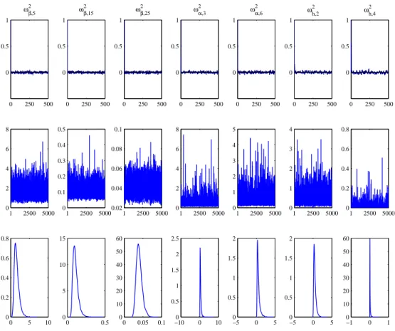
In Figure 2, we plot the sample autocorrelation function, the sample paths, and the poste- rior densities for selected parameters. The sample paths for each parameter look stable, and the sample autocorrelation function damps stably. In addition, the posterior densities show a single peaked pattern. Furthermore, Table 2 shows the estimates for posterior means, stan- dard deviations, the 95 percent credible intervals, the p-value of the convergence diagnostics (CD) of Geweke (1992), and inefficiency factors for selected parameters. Based on the CD statistics, the null hypothesis of the convergence to the posterior distribution is not rejected at the 5 percent significance level. These results suggest that the sample in our estimation is generated efficiently while being uncorrelated and adequately converged.
[Figure 2 about here.] [Table 2 about here.] 4.2. Stochastic volatility
Figure 3 depicts the posterior estimates of the volatilities of the reduced-form residuals (i.e., σit2 = exp(hit/2)). The solid line and the dotted lines indicate the median of the sampled volatility and the 68 percent credible intervals, respectively, while the shaded areas represent the ZLB periods. In Figure 3, it is worthwhile to mention that the volatility of the short- term interest rates is estimated to be almost zero during the ZLB periods. In addition, this observation is reported in Nakajima et al. (2011). Therefore, the zero restrictions on the
coefficients and the contemporaneous relation of the interest rate equation might be irrelevant for the estimation of volatility. At least, this small estimated volatility enables us to sample valid draws, even when imposing a strict non-negativity constraint on the short-term interest rates.
On the other hand, the volatility of the monetary base soared during the period in which an unconventional monetary policy was adopted. This implies that the monetary policy shock in the ZLB period played an important role in the variations of the monetary base. The finding that the volatility of short-term interest rates is low but that of the monetary base is high in the ZLB period justifies our identification strategy in which monetary policy shocks are characterized by combining sign restrictions on interest rates and the monetary base. Accordingly, this result implies that it is important to utilize the monetary base to capture the monetary policy shock when short-term interest rates hit the lower bound.
In addition, we observe that the volatility of government spending in the 1990s was rela- tively high compared with that after the 2000s. This is thought to reflect Japan’s aggressive fiscal policy implemented in the 1990s and its passive fiscal policy in the 2000s. Subsequently, the volatility of GDP seems to be stable before the Lehman Brothers shock, but shifts to a high level after the shock.
[Figure 3 about here.] 4.3. Impulse response functions
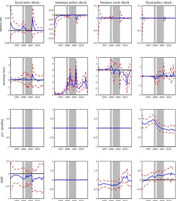
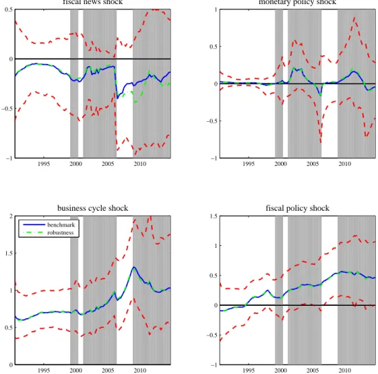
The IRFs of each variable to structural shocks are summarized in Figures 4 and 5. These figures show the contemporaneous and long-run effects (i.e., the effects 12 quarters after the shock) of four types of structural shocks on interest rates, monetary base, government spending, and GDP. The median responses and the 68 percent credible intervals are plotted by the solid and dotted lines, respectively, and the shaded areas indicates the ZLB periods. In Figure 4, which represents the impact responses, we can confirm that the contemporaneous responses of government spending to fiscal news, monetary policy, and business cycle shocks and those of GDP to monetary policy shocks are stuck on zero, based on the identification restriction. Moreover, the responses of interest rates to monetary policy shocks are restricted within the actual observed rates.
We first mention the effects of fiscal policy shocks shown in the fourth column of Figure 4. In both contemporaneous and long-run impacts, we can observe sign switches in the time variation of median responses of GDP. The signs of GDP to government spending shocks are negative (but insignificant) until the mid-1990s, and thereafter, change to positive until the end of the sample period. In particular, it is found that GDP significantly increases after the first half of the 2000s, when the BOJ started to adopt QE. From the viewpoint of fiscal and monetary interaction, a significant relationship between fiscal and monetary policies cannot be derived from our estimation owing to the wide credible intervals. However, from the time-varying responses of the monetary base to fiscal policy shocks, a structural change in the coordination between fiscal and monetary policies is observed at the timing of adoption of the zero interest rate policy. Apparently, the monetary base tends to respond greatly to the fiscal policy shock after the end of the 1990s although the direction of the responses is not unique. It is noteworthy that the sign of the median response in the monetary base to fiscal policy shocks changes from negative to positive in 2012Q4 when the Shinzo Abe administration took office. Furthermore, this positive response has been maintained under the Governor Haruhiko Kuroda of the Bank of Japan. Therefore, our results imply at least the possibility that fiscal and monetary policies after the adoption of the zero interest rate policy have some linkages, although the direction of the linkages varies over time. In addition, the recent form of the relationship is that the monetary authority has assumed an accommodative stance when positive fiscal policy has been enacted.
Next, we focus on the effects of monetary policy depicted in the second column of Figure 4. First, it is confirmed that the variation of the monetary base played an important role in monetary policy after short-term interest rates hit zero. On the contrary, the short-term interest rates hardly react to monetary policy shocks during the ZLB periods. This result indicates that monetary policy shocks under a zero interest rate cannot be captured only by using the short-term interest rates, and thus, justifies our identification strategy for monetary policy shocks. In Figure 5, the long-run responses of GDP to monetary policy shocks do not show significant results. In particular, the median responses of GDP before the adoption of the zero interest rate policy are almost zero. However, positive responses tend to be shown from the end of the 1990s, at least at the median value. This finding is consistent with the result reported in Honda et al. (2007), which is the representative research analyzing the
effects of QE in Japan.
Finally, we note the effects of fiscal news and business cycle shocks. Regarding fiscal news shocks, we do not obtain significant responses. In particular, the credible intervals of GDP response contain zero and the median responses take negative values over the sample period. In Section 5, we discuss what component contributes to the decrease of GDP by fiscal news shocks by estimating the same TVP-VAR model in which GDP is replaced with its components. On the other hand, with respect to business cycle shocks, we observe negative responses of the monetary base and government spending, and a positive response of GDP. This result can be interpreted as follows. The fiscal and monetary authorities automatically take a tight stance when a positive shock hits the economy in order to avoid overheating of the economy. This accords with our intuition, and thus, it can be said that the business cycle shock in this study is identified correctly.
[Figure 4 about here.] [Figure 5 about here.] 4.4. Fiscal multiplier
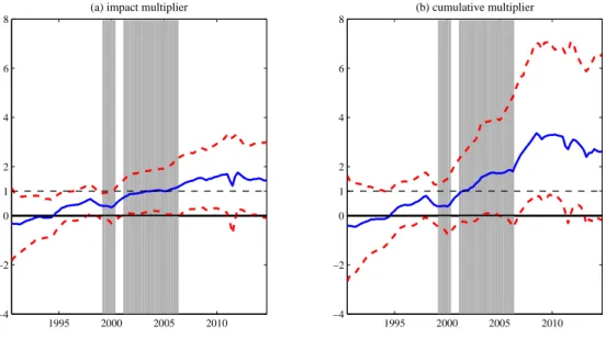
In Figures 4 and 5, we cannot compare the size of the effects of government spending shocks on GDP in each period because the size of government spending shocks varies over time. Figure 6 shows the estimates of time-varying fiscal multipliers for government spending shocks. Since the data for GDP and government spending in the VAR model are within the logarithms, the fiscal multiplier is computed as follows:
fiscal multipliert = IRF of GDPt
IRF of Gov. spendingt ×
GDPt
Gov. spendingt.
We calculate two types of fiscal multipliers: “impact” (Figure 6a), which uses impulse re- sponses during the impact period, and “cumulative” (Figure 6b), which uses the sum of the impulse responses for 12 quarters after the shock.
[Figure 6 about here.]
The figures show that both the impact and cumulative multipliers describe the same historical pattern. The median of the impact multiplier starting from a negative value grad- ually increases and exceeds 1 in the second half of the 2000s. The cumulative multiplier is
somewhat large compared with the impact multiplier and exceeds 1 in the first half of the 2000s.
As for fiscal policy shocks under the ZLB, our results reveal that the fiscal multiplier increases after the BOJ began to adopt the zero interest rate policy and QE. More precisely, we can observe that the impact multiplier takes significant positive values after the early 2000s, when the BOJ started QE policy. In addition, the cumulative multiplier exceeds 1 up to the end of the sample period after the adoption of QE. Because the short-term interest rates are sufficiently low from 2006Q2 to 2009Q1, in which the BOJ terminated the zero interest rate policy once, this result implies that the effects of government spending shocks are enhanced when short-term interest rates are extremely low. Therefore, our results empirically support the theoretical predictions of Braun and Waki (2006), Christiano et al. (2011), and Eggertsson (2010).
5. Robustness checks
5.1. Interest payments on bank reserves
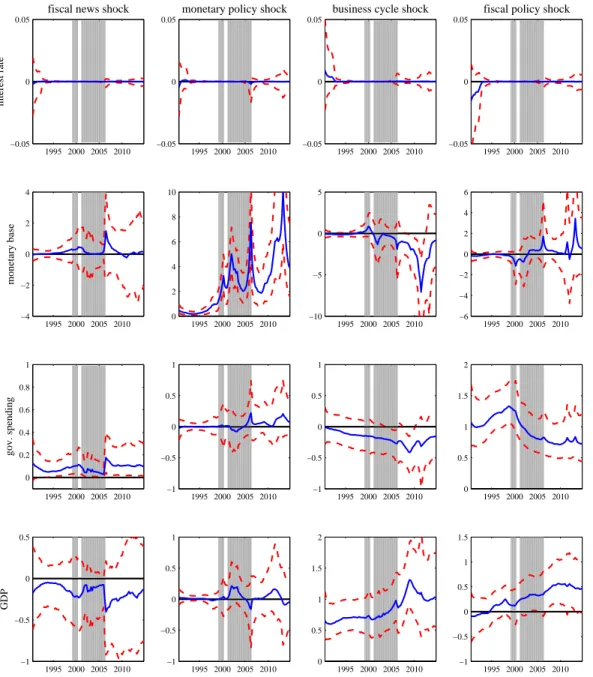
As noted in Hayashi and Koeda (2013), the BOJ has been paying interest rates on reserves since November 2008. Hence, the net policy rate, calculated by subtracting the rate paid on reserves (0.1% since 2008Q4) from the call rate, falls below 50 basis points in 2008Q4-2014Q4 in addition to the original definition of the ZLB period. In order to confirm the robustness of our results, we estimate the model under this new definition. Figures 7 and 8 depict the impacts and long-run effects of each structural shock on GDP, respectively. The blue solid lines and red dotted lines indicate the median responses and 68% credible intervals for the benchmark result, respectively, while the green dashed lines indicate the median responses under the new definition of the ZLB period. The shaded areas refer to the ZLB periods. As the figures show, the median responses in the robustness check almost exactly trail those in the benchmark. Therefore, we conclude that our benchmark result is robust irrespective of the definition of the ZLB period.
[Figure 7 about here.] [Figure 8 about here.]
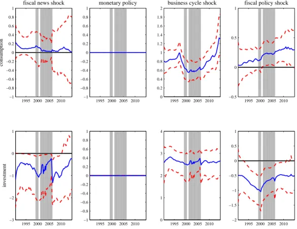
5.2. Components of GDP
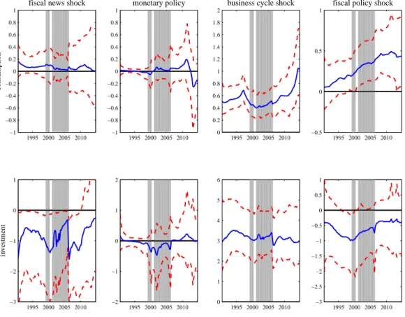
To understand the effects of each structural shock on GDP in detail, we estimate a model in which GDP is replaced with private consumption or private investment. Private consumption and investment are obtained from the SNA database. The aim of this exercise is to clarify which components contribute to the dynamic response of GDP. Figures 9 and 10 show the IRFs of consumption and investment to each shock in the impact period and long run. As in the previous figures representing the IRFs, the plotted series indicate the median responses and 68% credible intervals.
At first, regarding the responses to fiscal policy shocks, we confirm that the effects on consumption have been increasing significantly after the zero interest rate policy period. Unlike the responses of GDP, the median responses of consumption show significant positive signs over the sample period. On the other hand, investment seems to be crowded out by fiscal policy shocks. Hence, it is concluded that the positive responses of GDP to fiscal policy shocks stem from the positive responses of consumption. Moreover, our results imply the possibility that a rise of the effects of fiscal policy at the ZLB period is caused through the consumption channel.
In addition, the results reveal that negative responses of GDP to fiscal news shocks are dominated by large reductions of investment. Investment is strongly crowded out by fiscal news shocks. As opposed to investment, the responses of consumption show positive signs over the sample period, at least at the median estimates.
As for the responses to monetary policy shocks, we obtain no significant results as in GDP. However, the median responses show that unconventional monetary policy, like the zero interest rate policy and QE, exerted slightly negative effects on investment. In addition, it turns out that consumption in recent years responded to monetary policy shock negatively.
[Figure 9 about here.] [Figure 10 about here.]
6. Conclusion
This study investigated the effects of fiscal and monetary policy shocks in Japan by using the TVP-VAR model and accounting for the ZLB of nominal interest rates. In particular,
we focused on the effects of macroeconomic policies under the ZLB of nominal interest rates. We proposed a new identification method for unconventional monetary policies, in which we combined the methods presented by Nakajima (2011a) and sign restrictions. Furthermore, we calculated the fiscal multiplier throughout the sample period to confirm whether the effects of fiscal policy increased during the periods of the ZLB, as predicted by Braun and Waki (2006), Christiano et al. (2011), and Eggertsson (2010).
We summarize the main results as follows. First, the TVP-VAR-ZLB model can replicate the fact that the volatility of short-term interest rates becomes quite small during ZLB periods. This plays an important role in the ability to sample valid draws that satisfy non- negativity constraints on the short-term interest rates. In addition, during the period of QE, our estimated results capture the rise of volatility in the monetary base. Furthermore, the calculated IRFs imply that the effects of the fiscal and monetary policy shocks change over the sample period. The time-varying effects are observed in both the magnitude of the shocks and the transmission mechanism. Our result shows that fiscal policy shocks have significantly positive effects on GDP after adoption of unconventional monetary policy while fiscal news and monetary policy shocks have insignificant small effects on GDP. Moreover, for the responses to both fiscal policy shocks, it turns out that investment is crowded out. As for fiscal and monetary interaction, our results indicate the possibility that some linkages exist between these policies during ZLB periods. Finally, one of the principal findings of this study is that the effects of fiscal policy increase during ZLB periods in Japan. In addition, an increase in fiscal multipliers corresponding to fiscal policy during the ZLB periods is stemmed from a rise in the response of consumption.
Since several developed countries have experienced quite low interest rate policies, the estimation methodology presented in this study would be useful and applicable for analyses of those countries. In particular, it is important to clarify and reconcile the observed and theoretically predicted effects of fiscal policies during ZLB periods. Thus, it remains to be determined if our results are specific only to the particular economy of Japan.
References
Blanchard, O.J., Perotti, R., 2002. An empirical characterization of the dynamic effects of changes in government spending and taxes on output. Quarterly Journal of Economics
117(4), 1329-1368.
Braun, R.A., Waki, Y., 2006. Monetary policy during Japan’s lost decade. The Japanese Economic Review 57(2), 324-344.
Christiano, L.J., Eichenbaum, M., Evans, C.L., 1999. Monetary policy shocks: What have we learned and to what end? In: Woodford, Michael, Taylor, John (Eds.), Handbook of Macroeconomics, vol.1A. Elsevier Science, North-Holland, Amsterdam; New York and Oxford.
Christiano, L.J., Eichenbaum, M., Rebelo, S., 2011. When is the government spending mul- tiplier large? Journal of Political Economy 119(1), 78-121.
Durbin, J., Koopman, S.J., 2002. Simple and efficient simulation smoother for state space time series analysis. Biometrika 89(3), 603-616.
de Jong, P., Shephard, N., 1995. The simulation smoother for the time series models. Biometrika 82(2), 339-350.
Eggertsson, G.B., 2011. What fiscal policy is effective at zero interest rate? NBER Macroe- conomic Annual 2010, University of Chicago Press.
Franta, M., 2011. Identification of monetary policy shocks in Japan using sign restrictions within the TVP-VAR framework. IMES Discussion Paper No. 2011-E-13.
Fujiwara, I., 2006. Evaluating monetary policy when nominal interest rates are almost zero. Journal of the Japanese and International Economies 20(3), 434-453.
Fukuda, S-I., Yamada, J., 2011. Stock price targeting and fiscal deficit in Japan: Why did the fiscal deficit increase during Japan’s lost decades? Journal of the Japanese and International Economies 25(4), 447-464.
Gal´ı, J., L´opez-Salido, D., Vall´es, J., 2007. Understanding the effects of government spending on consumption. Journal of the European Economic Association 5(1), 227-270.
Gerba, E., Hauzenberger, K., 2014. Estimating US fiscal and monetary policy interactions: From Volcker chairmanship to the Great Recession. LSE Research Online Documents on Economics 56406, London School of Economics and Political Science, LSE Library.
Geweke, J., 1992. Evaluating the accuracy of sampling-based approaches to the calculation of posterior moments. J.M. Bernardo, J.O. Berger, A.P. Dawid, A.F.M. Smith (Eds.), Bayesian Statistics, vol. 4Oxford University Press, New York (1992), 169-188.
Hayashi, F., Koeda, J., 2013. A regime-switching SVAR analysis of quantitative easing. CARF Working paper, CARF-F322.
Honda, Y., Kuroki, Y., Tachibana, M., 2007. An injection of base money at zero interest rates: Empirical evidence from the Japanese experience 2001-2006. OSIPP Discussion Paper, 07-08.
Inoue, T., Okimoto, T., 2008. Were there structural breaks in the effects of Japanese mone- tary policy? Re-evaluating policy effects of the lost decade. Journal of the Japanese and International Economies 22(3), 320-342.
Kimura, T., Nakajima, J. 2013. Identifying conventional and unconventional monetary policy shocks: A latent threshold Approach. Bank of Japan Working Paper Series, No. 13-E-7. Kirchner, M., Cimadomo, J., Hauptmeier, S., 2010. Transmission of government spending
shocks in the Euro areas: Time variation and driving forces. Tinbergen Discussion Paper TI 2010-021/2.
Miyao, R., 2002. The effects of monetary policy in Japan. Journal of Money, Credit, and Banking 34(2), 376-392.
Mountford, A., Uhlig, H., 2009. What are the effects of fiscal policy shock? Journal of Applied Econometrics 24(6), 960-992.
Nakajima, J., 2011a. Monetary policy transmission under zero interest rates: An extended time-varying parameter vector autoregressive approach. The B.E. Journal of Macroeco- nomics 11(1), Article 32.
Nakajima, J., 2011b. Time-varying parameter VAR model with stochastic volatility: An overview of methodology and empirical applications. Monetary and Economics Studies 29, 107-142.
Nakajima, J., Kasuya, M., Watanabe, T., 2011. Bayesian analysis of time-varying parameter vector autoregressive model for the Japanese economy and monetary policy. Journal of the Japanese and International Economies 25(3), 225-245.
Pereira, M.C., Lopes, A.S., 2014. Time-varying fiscal policy in Japan. Studies in Nonliner Dynamics and Econometrics 18(2), 157-184.
Primiceri, G.E., 2005. Time varying structural vector autoregressions and monetary policy. The Review of Economic Studies 72(3), 821-852.
Ramey, V.A., 2011. Identifying government spending shocks: It’s all in the timing. Quarterly Journal of Economics 126(1), 1-50.
Rossi, B., Zubairy, S., 2011. What is the importance of monetary and fiscal shocks in ex- plaining U.S. macroeconomic fluctuations? Journal of Monetary, Credit and Banking 43(6), 1247-1270.
Shioji, E., 2000. Identifying Monetary Policy Shocks in Japan. Journal of the Japanese and International Economies 14(1), 22-42.
Uhlig, H., 2005. What are the effects of monetary policy on output? Results from an agnostic identification procedure. Journal of Monetary Economics 52(2), 381-419.
Watanabe, T., Omori, Y., 2004. A multi-move sampler for estimating non-Gaussian time series models: comments on Shephard and Pitt (1997). Biometrika 91(1), 246-248.
1995 2000 2005 2010 0
2 4 6 8 10
short−term interest rate
1995 2000 2005 2010
−15
−10
−5 0 5 10 15
monetary base
1995 2000 2005 2010
−4
−2 0 2 4
government spending
1995 2000 2005 2010
−4
−2 0 2 4
GDP
Figure 1: Data
0 250 500 0
0.5 1
ωβ,52
0 250 500
0 0.5 1
ωβ,152
0 250 500
0 0.5 1
ωβ,252
0 250 500
0 0.5 1
ωα,32
0 250 500
0 0.5 1
ωα,62
0 250 500
0 0.5 1
ωh,22
0 250 500
0 0.5 1
ωh,42
1 2500 5000 0
2 4 6 8
1 2500 5000 0
0.1 0.2 0.3 0.4 0.5
1 2500 5000 0.02
0.04 0.06 0.08 0.1
1 2500 5000 0
2 4 6 8
1 2500 5000 0
1 2 3 4 5
1 2500 5000 0
1 2 3 4
1 2500 5000 0
0.2 0.4 0.6 0.8
0 5 10
0 0.2 0.4 0.6 0.8
0 0.5
0 5 10 15
0 0.05 0.1 0
10 20 30 40 50 60
−100 0 10 0.5
1 1.5 2 2.5
−5 0 5
0 0.5 1 1.5 2
−5 0 5
0 0.5 1 1.5 2
−1 0 1
0 10 20 30 40 50 60
Figure 2: Estimation results for selected parameters
1995 2000 2005 2010 0
0.1 0.2 0.3 0.4 0.5 0.6
short−term interest rate
1995 2000 2005 2010 0
2 4 6 8
monetary base
1995 2000 2005 2010 0
0.5 1 1.5 2
government spending
1995 2000 2005 2010 0
0.5 1 1.5
GDP
Figure 3: Estimated volatility of reduced-form residuals
1995 2000 2005 2010
−0.05 0 0.05 0.1
interest rate
fiscal news shock
1995 2000 2005 2010
−0.25
−0.2
−0.15
−0.1
−0.05 0 0.05
monetary policy shock
1995 2000 2005 2010
−0.2
−0.1 0 0.1
business cycle shock
1995 2000 2005 2010
−0.2
−0.1 0 0.1
fiscal policy shock
1995 2000 2005 2010
−2
−1 0 1 2 3
monetary base
1995 2000 2005 2010 0
1 2 3 4 5 6
1995 2000 2005 2010
−4
−3
−2
−1 0 1 2
1995 2000 2005 2010
−4
−2 0 2 4
1995 2000 2005 2010
−1
−0.5 0 0.5 1
gov. spending
1995 2000 2005 2010
−1
−0.5 0 0.5 1
1995 2000 2005 2010
−1
−0.5 0 0.5 1
1995 2000 2005 2010 0
0.5 1 1.5 2
1995 2000 2005 2010
−1
−0.5 0 0.5
GDP
1995 2000 2005 2010
−1
−0.5 0 0.5 1
1995 2000 2005 2010 0
0.5 1 1.5 2
1995 2000 2005 2010
−1
−0.5 0 0.5 1
Figure 4: Contemporaneous impact of structural shocks on variables over time
1995 2000 2005 2010
−0.05 0 0.05
interest rate
fiscal news shock
1995 2000 2005 2010
−0.05 0 0.05
monetary policy shock
1995 2000 2005 2010
−0.05 0 0.05
business cycle shock
1995 2000 2005 2010
−0.05 0 0.05
fiscal policy shock
1995 2000 2005 2010
−4
−2 0 2 4
monetary base
1995 2000 2005 2010 0
2 4 6 8 10
1995 2000 2005 2010
−10
−5 0 5
1995 2000 2005 2010
−6
−4
−2 0 2 4 6
1995 2000 2005 2010 0
0.2 0.4 0.6 0.8 1
gov. spending
1995 2000 2005 2010
−1
−0.5 0 0.5 1
1995 2000 2005 2010
−1
−0.5 0 0.5 1
1995 2000 2005 2010 0
0.5 1 1.5 2
1995 2000 2005 2010
−1
−0.5 0 0.5
GDP
1995 2000 2005 2010
−1
−0.5 0 0.5 1
1995 2000 2005 2010 0
0.5 1 1.5 2
1995 2000 2005 2010
−1
−0.5 0 0.5 1 1.5
Figure 5: Long-run impact of structural shocks on variables over time
1995 2000 2005 2010
−4
−2 0 1 2 4 6 8
(a) impact multiplier
1995 2000 2005 2010
−4
−2 0 1 2 4 6 8
(b) cumulative multiplier
Figure 6: Contemporaneous and long-run fiscal multiplier over time
1995 2000 2005 2010
−1
−0.5 0 0.5
fiscal news shock
1995 2000 2005 2010
−1
−0.5 0 0.5 1
monetary policy shock
1995 2000 2005 2010
0 0.5 1 1.5 2
business cycle shock
benchmark robustness
1995 2000 2005 2010
−1
−0.5 0 0.5 1
fiscal policy shock
Figure 7: Contemporaneous impact of structural shocks on GDP over time - robustness check -
1995 2000 2005 2010
−1
−0.5 0 0.5
fiscal news shock
1995 2000 2005 2010
−1
−0.5 0 0.5 1
monetary policy shock
1995 2000 2005 2010
0 0.5 1 1.5 2
business cycle shock
benchmark robustness
1995 2000 2005 2010
−1
−0.5 0 0.5 1 1.5
fiscal policy shock
Figure 8: Long-run impact of structural shocks on GDP over time - robustness check -
1995 2000 2005 2010
−1
−0.8
−0.6
−0.4
−0.2 0 0.2 0.4 0.6 0.8 1
consumption
fiscal news shock
1995 2000 2005 2010
−1
−0.8
−0.6
−0.4
−0.2 0 0.2 0.4 0.6 0.8 1
monetary policy
1995 2000 2005 2010 0
0.2 0.4 0.6 0.8 1 1.2 1.4 1.6 1.8 2
business cycle shock
1995 2000 2005 2010
−0.5 0 0.5 1
fiscal policy shock
1995 2000 2005 2010
−3
−2
−1 0 1
investment
1995 2000 2005 2010
−1
−0.8
−0.6
−0.4
−0.2 0 0.2 0.4 0.6 0.8 1
1995 2000 2005 2010 0
1 2 3 4
1995 2000 2005 2010
−2
−1.5
−1
−0.5 0 0.5 1
Figure 9: Contemporaneous impact of structural shocks on consumption and investment over time