A General and Multi-lingual Phrase Chunking Model
Based on Masking Method
Yu-Chieh Wu1, Chia-Hui Chang1, and Yue-Shi Lee2
1Department of Computer Science and Information Engineering, National Central University, No.300, Jhong-Da Rd., Jhongli City, Taoyuan County 32001, Taiwan, R.O.C.
[email protected], [email protected]
2 Department of Computer Science and Information Engineering, Ming Chuan University, No.5, De-Ming Rd, Gweishan District, Taoyuan 333, Taiwan, R.O.C.
Abstract. Several phrase chunkers have been proposed over the past few years. Some state-of-the-art chunkers achieved better performance via integrating external resources, e.g., parsers and additional training data, or combining multiple learners. However, in many languages and domains, such external materials are not easily available and the combination of multiple learners will increase the cost of training and testing. In this paper, we propose a mask method to improve the chunking accuracy. The experimental results show that our chunker achieves better performance in comparison with other deep parsers and chunkers. For CoNLL-2000 data set, our system achieves 94.12 in F rate. For the base-chunking task, our system reaches 92.95 in F rate. When porting to Chinese, the performance of the base-chunking task is 92.36 in F rate. Also, our chunker is quite efficient. The complete chunking time of a 50K words document is about 50 seconds.
1 Introduction
Automatic text chunking aims to determine non-overlap phrases structures (chunks) in a given sentence. These phrases are non-recursive, i.e., they cannot be included in other chunks [1]. Generally speaking, there are two phrase chunking tasks, including text chunking (shallow parsing) [15], and noun phrase (NP) chuncking [16]. The former aims to find the chunks that perform partial analysis of the syntactic structures in texts [15], while the later aims to identify the initial portions of non-recursive noun phrase, i.e., the first level noun phrase structures of the parsing trees [17] [19]. In this paper, we extend the NP chunking task to arbitrary phrase chunking, i.e., base-chunking. In comparison, shallow parsing extracts not only the first level but also the other level phrase structures of the parsing tree into the flat non-overlap chunks.
Chunk information of a sentence is usually used to present syntactic relations in texts. In many Natural Language Processing (NLP) areas, e.g., chunking-based full parsing [1] [17] [24], clause identification [3] [19], semantic role labeling (SRL) [4], text categorization [15] and machine translation, the phrase structures provide down-stream syntactic features for further analysis. In many cases, an efficient and
high-performance chunker is required. In recent years, many high-performance chunking systems were proposed, such as, SVM-based [9], Winnow [13] [20], voted-perceptrons [3], Maximum Entropy model (ME) [12], Hidden Markov Model (HMM) [11] [14], Memory-based [17] [19], etc. Although some of the outstanding methods gave better results, they were not efficient. In average the chunking speed is about 3-5 sentences per second. Moreover, some of them require external resources, i.e., parser (Winnow[20]), and more training data (HMM[14]), or combining multiple learners (memory-based [19] and SVM-based [9]) to enhance chunking performance. However, the use of multiple learners does not only complicate the original system but also increase chunking time largely. In practice, external resources are not always available in many domains and languages. On the other hand, although some chunkers (e.g., HMM and memory-based chunkers), are quite efficient, they do not have exhilarating performances.
In this paper, we present a novel chunking method to improve the chunking accuracy. The mask method we propose is designed to solve the “unknown word problem” as many chunking errors occur due to unknown words. Imagine the cases when unknown words occur in the testing data, all lexical-related features, for example, unigram, can not be properly represented, thus the chunk type has to be determined by other non-lexical features. To remedy this, we propose a mask method to collect unknown word examples from the original training data. These examples are derived from mapping variant incomplete lexical-related features. By including these instances, the chunker can handle testing data, which contains unknown words. In addition, we also combine a richer feature set to enhance the performance. Based on the two constituents, the mask method and richer feature sets, higher performance is obtained. In the two main chunking tasks, our method outperforms the other famous systems. Besides, this model is portable to other languages. In the Chinese base-chunking task, our chunking system achieves 92.19 in F rate. In terms of time efficiency, our model is satisfactory, and thus able to handle the real-time processes, for example, information retrieval and real-time web-page translation. In a 500K words document, the complete chunking time is about 50 seconds.
The rest of this paper is organized as follows. Section 2 introduces the two main tasks: shallow parsing and base phrase chunking. Section 3 explains our chunking model. The mask method will be described in Section 4. Experimental results are showed in Section 5. Concluding remarks and future work are given in Section 6.
2 Descriptions of the Chunking Tasks
A chunk (phrase) is a syntactic structure, which groups several consecutive words to form a phrase. In this section, we define the two phrase chunking tasks, base-chunking and shallow parsing.
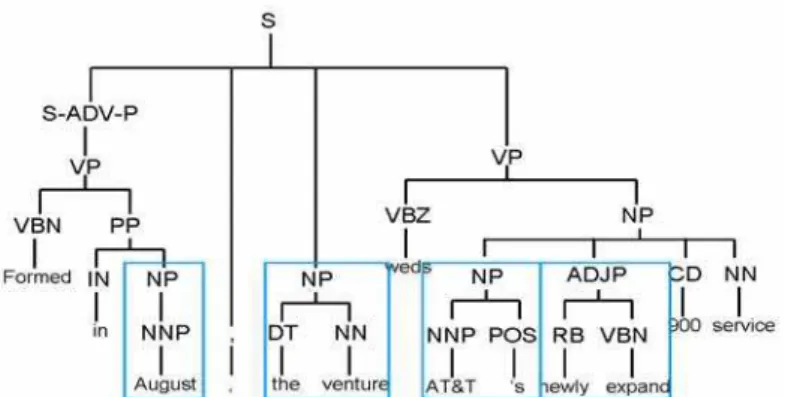
Fig. 1. A Parsing tree for “Formed in August, the venture weds AT&T ‘s newly expanded 900 service”
2.1 Base-Chunking
The phrase structures of base-chunking task is similar to that of baseNP chunking [16], but includes all atomic arbitrary phrase chunks in text. In Li and Roth’s works [13], they also compared their chunking system in the base-chunking tasks. Consider the following sentence: “Formed in August, the venture weds AT&T ‘s newly expanded 900 service”. As shown in Fig. 1, the parent node of each word (leaf node) is the part-of-speech (POS) tag. The first level chunks of the parsing tree are the pre-terminals that contain no sub-phrases. The base chunks of the above sentence are oval-shaped rectangles including “August”, “the venture”, “AT&T ‘s” and “newly expand”. The other phrase structures can not form the base chunk since they contain sub-phrases, for example, VP (verb phrase).
The phrase structures of the sentence can also be encoded using IOB2 style [18]. The major constituents of the IOB2 style are B/I/O tags and the phrase type, which represent the begin (B) of a phrase, the interior (I) of a phase and other words (O). For example, the chunk class of each token of the above sentence can be tagged as:
Formed (O) in (O) August (B-NP) , (O) the (B-NP) venture (I-NP) weds (O) AT&T (B-NP)
‘s (I-NP) newly (B-ADJP) expanded (I-ADJP) 900 (O) service (O)
When the chunk structure is encoded as IOB-like style, a chunking problem can be viewed as a word-classification task, i.e., identify IOB chunk tag for each word. Many chunkers [9] [13] [20] learn to label the IOB chunk tags using a classic classification scheme. We also follow the same scheme to design our model. More details of our model can be found in Section 3.
2.2 Shallow Parsing
Shallow parsing is also as known as text chunking which performs partial analysis of the parsing tree. It was the shared task of CoNLL-2000. The phrase structure of the shallow parsing is quite different from the base-chunking. Roughly speaking, in shallow parsing, a chunk contains everything to the left of and including the syntactic
head of the constituent of the same name. Shallow parsing focuses on dividing a text into phrases in such a way that syntactically related words become member of the same phrase type. So far, there are no annotated chunk corpora available which contain specific information about dividing sentences into chunks of words of variant phrase types. Thus, CoNLL-2000 [18] defines the shallow parsing phrase structures from parsing trees. Following the chunk definition in [18], the shallow parsing phrase structures are:
Formed (B-VP) in (B-PP) August (B-NP) , (O) the (B-NP) venture (I-NP) weds (B-VP) AT&T (B-NP) ‘s (I-NP) newly (B-ADJP) expanded (I-ADJP) 900 (B-NP) service (I-NP) In this case, even the term “Fomed” does not belong to the first level, it is specified as a verb phrase. A formal detail definition of the phrase structures of the shallow parsing can refer to the web site1 and literatures [18].
3 Chunking Model
As described in Section 2.1, the chunking problem can be viewed as a series of word-classification [13] [16]. Many common NLP components, for example Part-of-Speech (POS) taggers [7] and deep parsers [17] [19] were represented according to the “word-classification” structure. The proposed general chunking model is also developed following the same scheme. In general, the contextual information is often used as the seed feature type; the other features can then be derived based on the surrounding words. In this paper, we adopt the following feature types.
y Lexical information (Unigram) y POS tag information (UniPOS) y Affix (2~4 suffix and prefix letters) y Previous chunk information (UniChunk)
y Possible chunk classes for current word: For the current word to be tagged, we recall its possible chunk tags in the training data and use its possible chunk class as a feature.
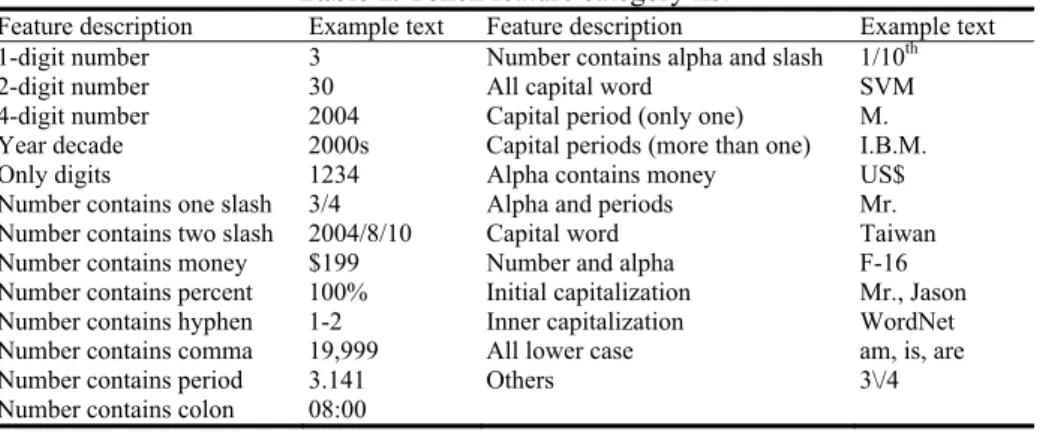
Additionally, we also add more N-gram features, including Bigram, BiPOS, BiChunk, and TriPOS. In addition, we design an orthographic feature type called Token feature, where each term will be assigned to a token class type via the pre-defined word category mapping. Table 1 lists the defined token feature types. Although this feature type is language dependent, many languages still contain Arabic numbers and symbols.
We employ SVMlight [8] as the classification algorithm, which has been shown to perform well on classification problems [7][8][15]. Since the SVM algorithm is a binary classifier, we have to convert it into several binary problems. Here we use the
“One-Against-All” type to solve the problem. To take the time efficiency into account, we choose the linear kernel type. As discussed in [7], working on linear kernel is
1 http://www.cnts.ua.ac.be/conll2000/chunking/
much more efficient than polynomial kernels. In Section 5, we also demonstrated that the training/testing time of the polynomial kernel is longer than linear kernels while causing a slight improvement.
Table 1. Token feature category list
Feature description Example text Feature description Example text 1-digit number 3 Number contains alpha and slash 1/10th
2-digit number 30 All capital word SVM
4-digit number 2004 Capital period (only one) M. Year decade 2000s Capital periods (more than one) I.B.M. Only digits 1234 Alpha contains money US$ Number contains one slash 3/4 Alpha and periods Mr. Number contains two slash 2004/8/10 Capital word Taiwan Number contains money $199 Number and alpha F-16 Number contains percent 100% Initial capitalization Mr., Jason Number contains hyphen 1-2 Inner capitalization WordNet Number contains comma 19,999 All lower case am, is, are Number contains period 3.141 Others 3\/4 Number contains colon 08:00
4 Mask Method
In real world, training data is insufficient, since only a subset of the vocabularies can appear in the testing data. During testing, if a term is an unknown word (or one of its context words is unknown), then the lexical related features, like unigram, and bigram are disabled, because the term information is not found in the training data. In this case, the chunk class of this word is mainly determined by the remaining features. Usually, this will low down the system performance.
The most common way for solving unknown word problem is to use different feature sets for unknown words and divide the training data into several parts to collect unknown word examples (Brill, 1995; Nakagawa et al., 2001; Gimenez & Marquez, 2003). However, the selection of these feature sets for known word and unknown word were often arranged heuristically and it is difficult to select when the feature sets are different. Moreover, they just extract the unknown word examples and miss the instances that contain unknown contextual words.
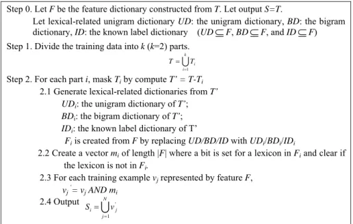
To solve this problem, the mask method is designed to produce additional examples that contain “weak” lexical information to train. If the classification algorithm can learn these instances, in testing, it is able to classify the examples, which contain insufficient lexical information. The mask method is described in Fig. 2. The method works as follows. First, the training data is divided into k non-overlapped partitions. For each partition, we create a mask, which is used to conceal part of the features for each example in the training set. New representations for each training example are generated, thus increasing the size of training set. The mask is created as follows. Suppose we have derived the feature dictionary, F, from the training set T. By remove partition i, we have a smaller training set with feature dictionary (Fi) smaller than F. We then generate new training examples by mapping the new dictionary set Fi, that is, lexicon-related features that do not occur in Fi are
masked. Technically, we create a mask mi of length |F| where a bit is set for a lexicon in Fi and clear if the lexicon is not in Fi. We then generate new vectors for all examples by logical “AND” it with mask mi. Thus, items which appear only in part i are regarded as unknown words. The process is repeated for k times and a total of (k+1)*N example vectors are generated (N is the original number of training examples). Computationally, we do not need to generate Fi from scratch. Instead, Fi can be created from F by replace lexicon-related features UDi, BDi, and IDi generated from T’, the training set except from partition i (since other non-lexicon related features are not masked).
Step 0. Let F be the feature dictionary constructed from T. Let output S=T.
Let lexical-related unigram dictionary UD: the unigram dictionary, BD: the bigram dictionary, ID: the known label dictionary (UD
⊆
F, BD⊆
F, and ID⊆
F) Step 1. Divide the training data into k (k=2) parts.Uk
i
Ti
T
=1
=
Step 2. For each part i, mask Ti by compute T’ = T-Ti
2.1 Generate lexical-related dictionaries from T’ UDi: the unigram dictionary of T’; BDi: the bigram dictionary of T’; IDi: the known label dictionary of T’
Fi is created from F by replacing UD/BD/ID with UDi/BDi/IDi
2.2 Create a vector mi of length |F| where a bit is set for a lexicon in Fi and clear if the lexicon is not in Fi.
2.3 For each training example vj represented by feature F, vj ‘= vj AND mi
2.4 Output
U
Nj j
i v
S
1 '
=
=
Step 3. S=S∪Si, Go to Step 1 until all parts has been processed
Fig. 2. The mask method to generate incomplete information examples
Let us illustrate a simple example. Assume that the unigram is the only one selected feature, and each training instance is represented via mapping to the unigram dictionary. At the first stage, the whole training data set generates the original unigram dictionary, T: (A,B,…,G). After splitting the training data (Step 1), two disjoint sub-parts are produced. Assume step 2.1 produces new unigram dictionaries, T1: (B,C,D,E) by masking the first part, and T2: (A,C,D,F,G) by masking the second part. Thus, the mask for the first partition is (0,1,1,1,1,0,0) which reserves the common items in T0 and T1. For a training example with features (A,C,F), the generated vectors is (C) since A and F are masked (Step 2.3). We use the same way to collect training examples from the second part.
The mask technique can transform the known lexical features into unknown lexical features and add k times training materials from the original training set. Thus, the original data can be reused effectively. As outlined in Fig. 2, new examples are generated through mapping into the masked feature dictionary set Fi. This is quite
different from previous approaches, which employed variant feature sets for unknown words. The proposed method aims to emulate examples that do not contain lexical information, since chunking errors often occur due to the lack of lexical features. Traditionally, the learners are given sufficient and complete lexical information; therefore, the trained models cannot generalize examples that contain incomplete lexical information. By including incomplete examples, the learners can take the effect of unknown words into consideration and adjust weights on lexical related features.
5 Experimental Results
In this section, four experiments are presented. First, we report the effects of various feature combinations, and the masking method on three chunking tasks, shallow parsing, base-chunking and Chinese base-chunking. Second, we compare our chunking performance to the other chunking systems using the same benchmarking corpus. The third experiment reports the detail performance on Chinese chunking task. The final experiments report the results using polynomial SVM kernel. The benchmarking corpus of the base-chunking is Wall Street Journal (WSJ) of the English Treebank, sections 02-21 for training and section 23 for testing. For the shallow parsing task, the WSJ sections 15-18 for training and 20 for testing. The POS-tag information of base-chunking and shallow parsing tasks is mainly generated from Brill-tagger [2]. However, in Chinese, there is no benchmarking POS-tagger. Thus, we use the gold POS-tags in Chinese Treebank.
The performance of the chunking task is measured by three rates, recall, precision, and F(β=1). CoNLL released a perl-script evaluator that enabled us to estimate the three rates automatically.
5.1 Analysis of Feature Combination and the Mask Method
There are three parameters in our chunking system: the context window size, the frequent threshold for each feature dictionary, and the number of division parts for the unknown word examples (N). We set the first two parameters to 2 as previous chunking systems [9]. Since the training time taken by SVMs scales exponentially with the number of input examples [8], we set N to 2 for all of the following experiments.
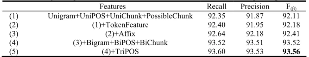
The first experiment reports the system performance of different feature combinations. Table 2 lists the chunking results of the added features on the shallow parsing task. For the feature set (4), which combines uni-gram and bi-gram features, it does a great improvement. On the contrary, the proposed “TokenFeature” marginally improves the performance. The best system performance is achieved by combining all of the features, i.e. feature set (5). The feature selection set in the following parts is (5).
In another experiment, we concern the performance of the mask method. Table 3 lists the improvement of the method. The mask method improves system performance
in different chunking tasks and different language. Note that there is not a public and well-known Chinese shallow parsing task definition. Thus, we did not perform the shallow parsing task on the Chinese Treebank.
Table 2. System performance on different feature sets in the shallow parsing task
Features Recall Precision F(β)
(1) Unigram+UniPOS+UniChunk+PossibleChunk 92.35 91.87 92.11
(2) (1)+TokenFeature 92.40 91.95 92.18
(3) (2)+Affix 92.64 92.18 92.41
(4) (3)+Bigram+BiPOS+BiChunk 93.52 93.51 93.52
(5) (4)+TriPOS 93.60 93.53 93.56
Table 3. The improvement by the mask method on Chinese and English corpus CoNLL-2000 Base-chunking Shallow-parsing
English 91.96 → 92.95 93.56 → 94.12 Chinese 91.76 → 92.36 N/A
The three statistical tests, s-test, probability distributional test, and McNemar’s test are applied to evaluate the improvement significance. Table 4 lists the results of the three tests. “P<0.01” means the two systems have statistical significant difference under the 99% confidence value. Three tests indicate that the mask method improves the chunking performance on these chunking tasks.
To exploit the detail performance analysis of the mask method, Table 5 shows the chunking performance on the known and unknown phrases. As listed in Table 5, the percentage of unknown phrases in the testing set is in the testing set is about 13.53% and the improvement for unknown words is from 89.84 to 90.84. The mask method improves a lot in the unknown phrase chunking. Moreover, the mask method also improves the chunking performance on known word. As discussed in Section 4, when unknown word appears, its lexical features are not available. The main idea of the mask method is to produce the training examples that contain incomplete lexical features. In testing phase, when the unknown word appears, the classification algorithm can identify the chunk class since it may “similar” to the incomplete training examples.
Table 4. Statistical significance test results
Chunking task System A System B s-test p-test M’s-test
Shallow parsing P<0.01 P<0.01 P<0.01
Base-chunking P<0.01 P<0.01 P<0.01
Chinese base-chunking
mask method Without mask method
P<0.01 P<0.01 P<0.01
Table 5. The improvement by the mask method Shallow-parsing Percentage Improvement Unknown 13.53% 89.84 → 90.84
Known 86.46% 94.34 → 94.76
Total 100.00% 93.56 → 94.12
5.2 Comparisons to Other Chunking Systems
In this section, we compare our model to currently state-of-the-art parsing systems [5] [6]. Here, we employed the Brill-tagger [2] to generate POS tags for our chunker and Collins’ parser. However, we do not feed the same POS tags to Charniak’s parser, since it takes the global optimize of the parsing tree structure into account. Table 6 lists the experimental results of each chunk type.
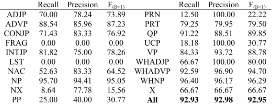
Table 6. Base-chunking performance of our model in different phrase type Recall Precision F(β=1) Recall Precision F(β=1) ADJP 70.00 78.24 73.89 PRN 12.50 100.00 22.22 ADVP 88.54 85.96 87.23 PRT 79.25 79.95 79.50 CONJP 71.43 83.33 76.92 QP 91.22 88.51 89.85
FRAG 0.00 0.00 0.00 UCP 18.18 100.00 30.77
INTJP 81.82 75.00 78.26 VP 84.33 93.72 88.78 LST 0.00 0.00 0.00 WHADJP 66.67 100.00 80.00 NAC 52.63 83.33 64.52 WHADVP 92.59 96.90 94.70
NP 95.70 94.41 95.05 WHNP 96.40 96.17 96.29
NX 8.64 77.78 15.56 X 66.67 66.67 66.67
PP 25.00 40.00 30.77 All 92.93 92.98 92.95
Table 7. Comparisons of chunking performance for base-chunking task Chunking system Recall Precision F(β)
This paper 92.93 92.98 92.95 Charniak’s full parser [5] 91.81 92.73 92.27 Collins’ full parser [6] 89.68 89.70 89.69
Table 8. Statistical significance test results System A System B s-test p-test M’s-test This paper Charniak P<0.01 P<0.01 P<0.01 This paper Collins P<0.01 P<0.01 P<0.01
Charniak Collins P<0.01 P<0.01 P<0.01
Table 7 reports the base-chunking results of the other famous parsing systems, Charniak’s maximum entropy inspired parser [5] and the Collins’ headword-driven parser [6]. Among the three systems, the Charniak’s parser performs the second best on the base-chunking tasks while the Collins parser achieves the third best performance. The three statistical tests, s-test, probability distributional test, and McNemar’s test again agree with the significant difference between our model and the two parsers under the 99% confidence score. Table 8 displays the statistical test results.
In the shallow parsing task, we compare our chunker with other chunking systems under the same constraint, i.e. all of the settings should be coincided with the CoNLL-2000 shared task. In other words, the use of external resources or other components is disabled. Table 9 lists our chunking results on each chunk type.
Table 10 reports the chunking results of other systems. In this test, the second best chunking system is the voted-SVMs [9]. As listed in Table 10, our model outperforms
the other chunking systems. However, it is difficult to perform the statistical tests on these chunkers. Since the outputs of these systems are not available easily.
Table 9. Shallow parsing performance of our model in different phrase type
Recall Precision F(β=1) Recall Precision F(β=1)
ADJP 71.92 81.61 76.46 NP 94.51 94.67 94.59 ADVP 81.64 83.27 82.45 PP 98.27 96.87 97.57 CONJP 55.56 45.45 50.00 PRT 79.25 76.36 77.78
INTJP 50.00 100.00 66.67 SBAR 86.54 87.86 87.19 LST 0.00 0.00 0.00 VP 94.57 94.10 94.34
All 94.12 94.13 94.12
Table 10. Comparison of chunking performance for text-chunking task
Chunking system Recall Precision F(β) This paper 94.12 94.13 94.12 Voted-SVMs [9] 93.89 93.92 93.91 Voted-perceptrons [3] 94.19 93.29 93.74 Generalized Winnow [20] 93.60 93.54 93.57
5.3 Experimental Results on Chinese Base-Chunking Tasks
We port our chunker into Chinese base-chunking task with the same parameter settings. There are about 0.4 million words in the Chinese Treebank. The front part of 0.32 million words forms the training data while the other 0.08 million words as the testing part. The ratio of training and testing data is equivalent to 4:1. Table 11 lists the experimental results of the Chinese base-chunking task.
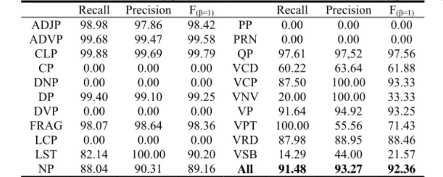
Table 11. Chinese base-chunking performance of our model in different phrase type
Recall Precision F(β=1) Recall Precision F(β=1) ADJP 98.98 97.86 98.42 PP 0.00 0.00 0.00 ADVP 99.68 99.47 99.58 PRN 0.00 0.00 0.00 CLP 99.88 99.69 99.79 QP 97.61 97,52 97.56
CP 0.00 0.00 0.00 VCD 60.22 63.64 61.88 DNP 0.00 0.00 0.00 VCP 87.50 100.00 93.33
DP 99.40 99.10 99.25 VNV 20.00 100.00 33.33 DVP 0.00 0.00 0.00 VP 91.64 94.92 93.25 FRAG 98.07 98.64 98.36 VPT 100.00 55.56 71.43 LCP 0.00 0.00 0.00 VRD 87.98 88.95 88.46 LST 82.14 100.00 90.20 VSB 14.29 44.00 21.57 NP 88.04 90.31 89.16 All 91.48 93.27 92.36
It is worth to note that the affix feature in the Chinese base-chunking task is not explicitly. Therefore, we use the atomic Chinese characters to form the affix feature. Although, several Chinese shallow parsing systems were proposed in recent years, like HMM-based [11] and maximum entropy-based [12] methods. It is difficult to compare with these chunkers, because there is not a standard benchmark corpus and grammar rules to represent the shallow parsing structures. Nevertheless, they were performed on different training and testing set and employed various pre-defined
grammar rules. Thus, we only report the actual results of the proposed chunking model for Chinese base-chunking task.
5.4 Working on polynomial kernel
Previous studies [7] indicated that using polynomial kernel to SVM is more accurate than linear kernel but cause much time cost. In this section, we report the performance of our method using polynomial kernel instead of the linear kernel. Table 12 lists the chunking results on the English shallow parsing task. In this experiment, the training time is about 4 days, besides it took 3 hours for chunking. Although the use of polynomial kernel improves the performance, the time cost is largely increased. When working on linear kernel, the training time of our model is less than 2.8 hours and 50 seconds for testing. The three statistical tests disagree with the significant difference between the two kernels in 95% confidence score.
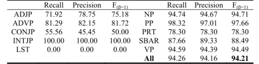
Table 12. Shallow parsing performance of our model using polynomial kernel Recall Precision F(β=1) Recall Precision F(β=1)
ADJP 71.92 78.75 75.18 NP 94.74 94.67 94.71 ADVP 81.29 82.15 81.72 PP 98.32 97.01 97.66 CONJP 55.56 45.45 50.00 PRT 78.30 78.30 78.30 INTJP 100.00 100.00 100.00 SBAR 87.66 89.33 88.49
LST 0.00 0.00 0.00 VP 94.59 94.39 94.49
All 94.26 94.16 94.21
6 Conclusion
This paper proposes a general and language dependent chunking model based on combining rich features and the proposed mask method. In the two main chunking tasks (shallow parsing and base-chunking), our method outperforms the other systems which employed more training materials or complex models. The statistical tests also report the proposed mask method significantly improves the system performance under a 99% confidence score. The online demonstration of our chunkers can be found at (http://140.115.155.87/bcbb/chunking.htm).
Acknowledgement
This work is sponsored by National Science Council, Taiwan under grant NSC94-2524-S-008-002.
References
1. Abney, S.: Parsing by chunks. In Principle-Based Parsing. Computation and Psycholinguistics (1991) 257-278.
2. Brill, E.: Transformation-based error-driven learning and natural language processing: a case study in part of speech tagging. Computational Linguistics (1995) 21(4):543-565.
3. Carreras, X. and Marquez, L.: Phrase recognition by filtering and ranking with perceptrons. Proceedings of the International Conference on Recent Advances in Natural Language Processing (2003).
4. Carreras X. and Marquez, L.: Introduction to the CoNLL-2004 shared task: semantic role labeling. Proceedings of Conference on Natural Language Learning (2004) 89-97.
5. Charniak, E.: A maximum-entropy-inspired parser. Proceedings of the ANLP-NAACL (2000) 132-139.
6. Collins, M.: Head-driven statistical models for natural language processing. Ph.D. thesis. University of Pennsylvania (1998).
7. Giménez, J. and Márquez, L.: Fast and accurate Part-of-Speech tagging: the SVM approach revisited. Proceedings of the International Conference on Recent Advances in Natural Language Processing (2003) 158-165.
8. Joachims, T.: A statistical learning model of text classification with support vector machines. In Proceedings of the 24th ACM SIGIR Conference on Research and Development in Information Retrieval (2001) 128-136.
9. Kudoh, T. and Matsumoto, Y.: Chunking with support vector machines. Proceedings of the 2nd Meetings of the North American Chapter and the Association for the Computational Linguistics (2001).
10. Li, H., Huang, C. N., Gao, J. and Fan, X.: Chinese chunking with another type of spec. The Third SIGHAN Workshop on Chinese Language Processing (2004).
11. Li, H., Webster, J. J., Kit, C. and Yao, T.: Transductive HMM based chinese text chunking. International Conference on Natural Language Processing and Knowledge Engineering (2003) 257-262.
12. Li, S. Liu, Qun, and Yang, Z.: Chunking based on maximum entropy. Chinese Journal of Computer (2003) 25(12): 1734-1738.
13. Li, X. and Roth, D.: Exploring evidence for shallow parsing. In Proceedings of Conference on Natural Language Learning (2001) 127-132.
14. Molina, A. and Pla, F.: Shallow parsing using specialized HMMs. Journal of Machine Learning Research (2002) 2:595-613.
15. Park, S. B. and Zhang, B. T.: Co-trained support vector machines for large scale unstructured document classification using unlabeled data and syntactic information. Journal of Information Processing and Management (2004) 40: 421-439.
16. Ramshaw, L. A. and Marcus, M. P.: Text chunking using transformation-based learning. Proceedings of the 3rd Workshop on Very Large Corpora (1995) 82-94.
17. Tjong Kim Sang, E. F.: Transforming a chunker to a parser. In Computational Linguistics in the Netherlands (2000) 177-188.
18. Tjong Kim Sang , E. F. and Buchholz, S.: Introduction to the CoNLL-2000 shared task: chunking. In Proceedings of Conference on Natural Language Learning (2000) 127-132. 19. Tjong Kim Sang, E. F.: Memory-based shallow parsing. Journal of Machine Learning
Research (2002) 559-594.
20. Zhang, T., Damerau, F., and Johnson, D.: Text Chunking based on a Generalization Winnow. Journal of Machine Learning Research (2002) 2:615-637.