Slip Suppression Sliding Mode Control with
Various Chattering Functions
Shun Horikoshi, Tohru Kawabe
Abstract—This study presents performance analysis results of SMC (Sliding mode control) with changing the chattering functions applied to slip suppression problem of electric vehicles (EVs). In SMC, chattering phenomenon always occurs through high frequency switching of the control inputs. It is undesirable phenomenon and degrade the control performance, since it causes the oscillations of the control inputs. Several studies have been conducted on this problem by introducing some general saturation function. However, study about whether saturation function was really best and the performance analysis when using the other functions, weren’t being done so much. Therefore, in this paper, several candidate functions for SMC are selected and control performance of candidate functions is analyzed. In the analysis, evaluation function based on the trade-off between slip suppression performance and chattering reduction performance is proposed. The analyses are conducted in several numerical simulations of slip suppression problem of EVs. Then, we can see that there is no difference of employed candidate functions in chattering reduction performance. On the other hand, in slip suppression performance, the saturation function is excellent overall. So, we conclude the saturation function is most suitable for slip suppression sliding mode control.
Keywords—Sliding mode control, chattering function, electric vehicle, slip suppression, performance analysis.
I. INTRODUCTION
I
N this century, automobiles have become popular all over the world and the number of automobiles has been increasing rapidly, especially in the developing countries. With such wide spread of internal-combustion engine vehicles (ICEVs) all over the world, the environment and energy problems: air pollution, global warming, and so on, are going severely [1]. In this situation, therefore, the development of next-generation vehicles, for example, electric vehicles (EVs) and so on, is very important. EVs run are zero emission and eco-friendly. So EVs have attracted great interests as one of the powerful solution against the problems mentioned above [2].EVs are driven by electric motors and electric motors have several advantages over ICEs:
1) The motor torque response between input and output is hundreds of times faster than that of gasoline/diesel engines.
2) Since we can detect the wheel torque in EV accurately and easily, it is possible to accurate and quick drive control for EV. On the other hands, the wheel torque of ICEV has high-nonlinearity due to the temperature
S. Horikoshi was with Department of Computer Science, Graduate School of Systems and Information Engineering, University of Tsukuba, Tsukuba 305-8573 Japan.
T. Kawabe is with the Division of Information Engineering, Faculty of Engineering, Information and Systems University of Tsukuba, Tsukuba 305-8573 Japan (phone: +81-29-853-5507; e-mail: kawabe@cs.tsukuba.a.jp).
and revolutions. Therefore, it’s difficult to measure the accurate value of the torque in ICEVs. However, the value of motor torque is surveyed easily and accurately from
3) The vehicle bodies can be made smaller by using multiple motors set into each wheels, if each wheels can be controlled to drive independently.
There have been several research results about various vehicle control methods, e.g., Anti-lock-Braking
Systems (ABS), Traction-Control-Systems (TCS),
Electric-Stability-Control (ESC) [3], Vehicle-Stability-Assist (VSA) [4], All-Wheel-Control (AWC) [5], and so on. The objective of these methods in common is to maintain a suitable tire grip margin and to improve the driving performance. But, the response time between the driving torque input and the tire force transmitted to the wheels is slow in the case of vehicles with gasoline/diesel engines. Therefore such vehicles limit the control performance.
On the other hands, EVs have a fast torque response and the motor characteristics can be used to accurately determine the torque, which makes it relatively easy and inexpensive to realize high-performance traction control. Then, several methods have been proposed for the traction control [6]-[8] by using slip ratio of EVs, such as the method based on Model Following Control (MFC) in [6]. We have been proposed conventional Sliding Mode Control (SMC) based method [9]. However, for slip suppression with the conventional SMC [10], the control performance will get degradation due to the chattering which always occurs when switching the control inputs due to the structure of SMC. To overcome such disadvantages, we have also proposed the extended SMC method, so-called SMC-I, introducing the integral action with gain to design the sliding surface in [11]. Although we employ the general saturation function for chattering reduction in this method, the performance could not be enough. In order to get better control performance, we need to solve such problem.
This paper, therefore, several candidate functions for chattering reduction are selected and control performance of SMC with candidate functions is analyzed. In the analysis, evaluation function based on the trade-off between slip suppression performance and chattering reduction performance is proposed. The analyses are conducted in several numerical simulations of slip suppression problem of EVs.
II. SLIDINGMODECONTROL
A. Basic Concept of SMC
SMC (sliding Mode Control) is one of the VSC (Variable Structure Control) methodsin 1970’s [12], [13]. From 1980’s,
with the improvement of computer performance, SMC is applied in many control fields such as high-precision motor control [14], automotive control [15] and robot attitude control [16]. Now SMC is considered as an effective nonlinear-robust control method and have been attracted more and more attention. SMC utilizes discontinuous feedback control laws to force the system trajectory to reach, and subsequently to remain on a specified surface within the state space (it’s so called sliding or switching surface). For example, consider the single input nonlinear system [17].
x(n)= f(x) +b(x)u (1) where u is the control input and x= [x x˙ ... x(n−1)]T is
the state vector. In general, the function f(x)and the control gainb(x)are nonlinear. In (1), f(x)andb(x)are not exactly known, but the extents of the imprecision on f(x) and b(x)
are upper bounded by known continuous functions of x. The control problem is to seek a control law that makes the state
xto track the desired statex∗= [x∗ x˙∗ ... x∗(n−1)]T in the
presence of model imprecision on f(x)andb(x).
Let us define a time-varying surfaceS(t)in the state space
R(n) by the equation s(x;t)defined as follow,
S(t) =
x|s(x;t) =0 (2) where s(x;t)is defined by
s(x;t) =d
dt+α
n−1
xe, α>0 (3)
wherexe=x−x∗= [xe x˙e ... xe(n−1)]T indicates the error
between the output state and the desired one. The tracking problem of x≡x∗ is equivalent to remain on the surfaceS(t)
for all t>0. From (3), s≡0 presents a linear differential equation whose unique solution is xe≡0. Thus, the problem of tracking the n-dimensional vector x∗ can be replaced by a 1st order stabilization problem in s. Whens(x;t)equals 0, that is to say, the system trajectories reach the surface which represents the tracking error is 0. Here, S(t) is known as sliding surface. On this surface, the error will converge to 0 exponentially.
B. Implementation of SMC
In general, to design a control system based on SMC should go through the following two steps:
• Design a sliding surface that is invariant of the controlled dynamics.
• Define the control input that drives the system trajectory to the sliding surface in sliding mode in finite time. Considering the system equation (1) defined in the previous section, assume that for all x,b(x)=0. We derive a control such that ˙s=0 when the sliding mode exists, (3) can be rewrite as
s=x(n−e 1)+...+αn−1xe. (4)
Differentiate equation (4), we can obtain that
˙
s = x(n)e +...+αn−1x˙e
= x(n)−x∗(n)+...+αn−1x˙e
= f(x) +b(x)u−x∗(n)+...+αn−1xe˙ (5)
while the dynamics is in sliding mode,
˙
s=0. (6)
By solving the equation for the control input,u=ueq,
ueq= 1
b(x)
−f(x) +x∗(n)−...−αn−1xe˙. (7) Here,ueq is called the equivalent control input, which can
be interpreted as the control law that would maintain ˙s=0 if the dynamics were in the sliding mode. However, if the system trajectory is not on the sliding surface (the reaching mode), an another item has to be added to the control input to drive the system to the sliding surface. In the reaching mode, the switching controlusw makes the trajectory from the initial trajectory to the sliding surface and it can be defined as
usw=− K
b(x)sgn(s) (8)
where
sgn(s) =
⎧
⎪ ⎪ ⎪ ⎪ ⎨
⎪ ⎪ ⎪ ⎪ ⎩
−1, s<0
0, s=0 1, s>0
(9)
andK is called sliding gain.
In (8), the switching control using the discontinuous function requires infinitely fast switching, but in real systems, the sampling and delays in digital implementation causessto pass to the other side of the surface S(t), which produces chattering. Chattering is high-frequency finite oscillations which is caused by switching of the variable s around the sliding surface S(t). That’s the point. For reducing the chattering, it is conceivable to adopt a function sat(s
Φ) is
defined as
sat s
Φ
=
⎧
⎪ ⎪ ⎪ ⎪ ⎪ ⎨
⎪ ⎪ ⎪ ⎪ ⎪ ⎩
−1, s<−Φ
s
Φ, −Φ≤s≤Φ
1, s>Φ
(10)
where Φ>0 is a design parameter representing the width of the boundary layer around the sliding surfaces=0. With this replacement, the sliding surface function swith an arbitrary initial value will reach and stay within the boundary layer |s| ≤Φ.
From (8), the switching control is rewritten as
usw=− K b(x)sat
s
Φ
. (11)
Finally, the SMC control law can be defined as
u = ueq+usw
= −1
b(x)
f(x)−x∗(n)+...+αn−1x˙
e+Ksat
s
Φ
.(12)
In summary, when the trajectory is on the sliding surface (s=0), it is desired to haveusw=0, the switching control has
no effect on the sliding surface. Moreover, when the trajectory
is off the sliding surface or the uncertainty in the system occurs, the switching control acts to return the trajectory back to the sliding surface. Therefore, the total controlucauses the system to keep the trajectory on the sliding surface.
III. ELECTRICVEHICLEDYNAMICS
A. One Weel Car Model
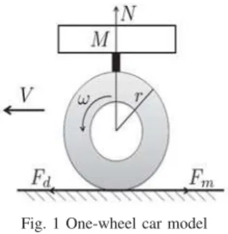
As a first step toward practical application, this paper restricts the vehicle motion to the longitudinal direction and uses direct motors for each wheel to simplify the one-wheel model to which the drive force is applied. In addition, braking was not considered this time with the subject of the study being limited to only when driving.
Fig. 1 One-wheel car model
From Fig. 1, the vehicle dynamical equations are expressed as (13)-(15).
MdV
dt = −Fd(λ) +Fa (13) Jdω
dt = rFd(λ)−Tb (14) Fd = µ(c,λ)N (15)
whereMis the vehicle weight,V is the vehicle body velocity,
Fd is the driving force, J is the wheel inertial moment, Fa
is the resisting force from air resistance and other factors on the vehicle body, Tb is the braking torque, ω is the wheel
angular velocity, r is the wheel radius, c is road surface condition coefficient, and λ is the slip ratio. The slip ratio of the wheel is defined as the difference between the wheel and body velocities, divided by the maximum of these velocity values (wheel velocity for acceleration, vehicle body velocity for braking), and given by
λ=
⎧
⎪ ⎪ ⎪ ⎨
⎪ ⎪ ⎪ ⎩
Vω−V Vω
(accelerating)
V−Vω
V (braking)
(16)
The value of λ =0 characterizes the free motion of the wheel where no wheel slip happens (no friction force is exerted). If the slip attains the value λ =1, then the wheel is completely skidding. The friction forces that are generated between the road surface and the tires are the force generated in the longitudinal direction of the tires and the lateral force acting perpendicularly to the vehicle direction of travel, and both of these are expressed as a function of λ. The friction force generated in the tire longitudinal direction is expressed
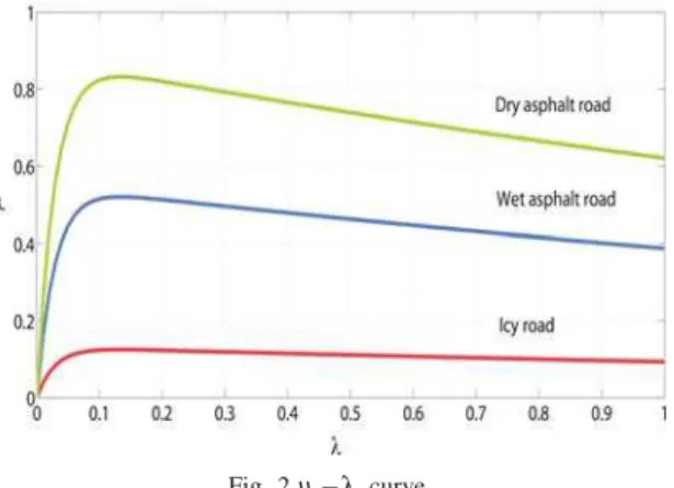
as µ, and the relationship between µ and λ is shown by (17) below, which is a formula called the Magic-Formula
and gives values compatible with experimental data given in [18]. It is simplified and has been using in earlier study in [19].
µ(c,λ) = −c×1.1×
e−35λ−e−0.35λ (17)
wherecis the coefficient used to determine the road condition and was found by experimental data to be approximatelyc=
0.8 for general dry asphalt roads, approximately c=0.5 for general wet asphalt roads, and approximatelyc=0.12 for icy road. In the simulations, this formula is used for estimating the maximum value of friction coefficient.
Theµ−λ curve for acceleration case is shown in Fig. 2 on three different road conditions (dry asphalt, wet asphalt and icy road). It shows how the friction coefficient µ increases with slip ratioλ up to a valueλ∗ (0.1<λ∗<0.2) where it attains
the maximum value of the friction coefficient. As defined in (15), the driving force also achieves the maximum value in corresponding to the friction coefficient. However, the friction coefficient decreases to the minimum value when the wheel is completely skidding. Therefore, to achieve the maximum value of driving force for slip suppression,λ should be maintained at the desired valueλ∗. The value ofλ∗is derived as follows.
Choose the functionµc(λ)defined as µc(λ) =−1.1×
e−35λ−e−0.35λ. (18)
By using equation (18), Equation (17) can be rewritten as
µ(c,λ) =c·µc(λ). (19)
Evaluating the values of λ which maximize µ(c,λ) for different c(c>0), means to seek the value of λ where the maximum value of the function µc(λ)can be obtained. Then
let
d
dλµc(λ) =0 (20)
and solving equation (20) gives
λ= log100
35−0.35 ≈ 0.13. (21)
Therefore, for the different road conditions, whenλ≈0.13 is satisfied, the maximum driving force can be gained. Namely, from (17) combined with Fig. 2 we find that regardless of the road condition (value ofc ), theµ−λ surface attains the largest value ofµ whenλ is the optimal value 0.13. So in this dissertation, desired value of slip ratio is set by λ∗=0.13.
IV. SMCWITHINTEGRALACTION FORSLIPSUPPRESSION
In this section, the previous proposed control strategy based on SMC with integral action (SMC-I) [11] is explained. Without loss of generality, one wheel car model in Fig. 1 is used for the design of the control law. The nonlinear system dynamics can be presented by a differential equation as
˙
λ=f+bTm (22)
where λ ∈R is the state of the system representing the slip ratio of the driving whee which is defined as (16) for the
Fig. 2µ−λ curve
case of acceleration, Tm∈Ris the control input representing
the torque of the motor. f describes the nonlinearity of system and bis the input gain, and they are all time-varying. Differentiating (16) for the case of acceleration with respect to time gives
˙
λ=−V˙+ (1−λ)Vw˙
Vw
(23)
Then, the system dynamics can be rewritten as
˙
λ=− g
Vw
1+ (1−λ)r
2M
Jw
µ(c,λ) +(1−λ)r
JwVw
Tm. (24)
By reference to the system dynamics, the following equations can be attained,
f = − g
Vw
1+ (1−λ)r
2M
Jw
µ(c,λ), (25)
b = (1−λ)r
JwVw
. (26)
The sliding mode controller is described to maintain the value of slip ratio λ at the desired valueλ∗.
Referring to [11], in order to reduce the undesired chattering effect for which it is possible to excite high frequency modes, and guarantee zero steady-state error, an integral action with gain has been introduced to the design of sliding surface. By adding an integral item to the difference between the actual and desired values of the slip ratio, the sliding surface function
sis given by
s=λe+Kin
t
0
λe(τ)dτ, (27)
whereλeis defined asλe=λ−λ∗andKinis the integral gain, Kin>0.
The sliding mode occurs when the state reaches the sliding surface defined by s=0. The dynamics of sliding mode is governed by
˙
s=0. (28)
By using (22)-(28), the sliding mode control law is derived by adding a switching control input Tmsw to the nominal
equivalent control inputTmeq n as in [11]
Tm=Tmeq n+Tmsw, (29)
Tmeq n=
1
b[−fn−Kinλe], (30) Tmsw=
1
b
−Ksat(s
Φ)
, (31)
where “n” is used to indicate the estimated model parameters. fnis the estimation of f calculated by using the nominal values
of vehicle massMn and road surface condition coefficientcn. Φ>0 is a design parameter which defines a small boundary layer around the sliding surface. The sliding gain K>0 is selected as
K=F+η (32)
by defining Lyapunov candidate function in [11], whereF=
|f−f n|andη is a design parameter.
By using (29), (30), (31) and (32), the control law of SMC-I can be represented as
Tm=
1
b
−fn−Kinλe−(F+η)sat
s
Φ
. (33)
In this method, standard saturation function, sats
Φ
in (10), was employed.
V. ANALYSIS OFCONTROLPERFORMANCE
A. Candidates for Chattering Function
The switching control input using the sign function in (9) is used theoretically. But, in real systems, the sampling and delays in digital implementation causessto pass to the other side of the surfaceS(t), which produces chattering. A solution to reduce this chattering introduces a region around S(t)
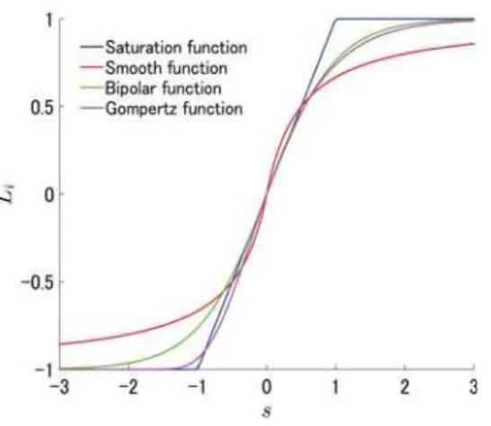
called boundary layer so thatschanges its value continuously [17]. The boundary layer is realized to use “S-shape type” function replacing sgn(s). Since the trajectory in the boundary layer varies depend on the used function, the chattering reduction performance is different. Hereinafter the function of the S-shape type used for boundary layer introduction is called the chattering reduction function. In this paper,L0,L1,
L2 andL3 shown in (37) are considered as candidates of the chattering function,
L0 = ⎧
⎪ ⎨
⎪ ⎩
−1 (s<−Φ)
s
Φ (−Φ≤s≤Φ)
1 (s>Φ)
(34)
L1 =
s
|s|+δ (35)
L2 = tanh σs
2
(36)
L3 = 2×
1 2
bs
−1 (37)
where Φδ σb(0<b<1)are design parameters related to the width of boundary layer.
L0 is Saturation function, and it’s same as (10). In this function, the width of the boundary layer becomes narrow so as to smaller the value of Φ. L1 is Smooth function. In this function, the width of the boundary layer becomes narrow so as to smaller the value of δ. L2 is Bipolar function. In this function, the width of the boundary layer becomes narrow so
Fig. 3 Candidate functions
as to bigger the value of σ.L3 is Gompertz function and its asymmetry. In this function, the width of the boundary layer becomes narrow so as to smaller the value ofb. The chattering reduction performance of these four functions are analyzed. These four functions are shown in Fig. 3. Values of parameters in each function are tuned asΦ=1.0,δ=0.5,σ=2.0,b=0.2 for visibility.
B. Evaluation Index for Control Performance
The index to compare the performance of 4 candidate functions is considered. It can be said that there is generally a relation of a trade-off in the slip suppression performance and the chattering reduction performance in slip suppression problem by using SMC. Therefore, it is desirable to reduce chattering of the driving torque without deteriorating slip suppression performance. From this fact, the following evaluation index is introduced.
J=kcC+keE (38)
where C=max
dTm dt
, E=
tf
0 |
˜
λ|dt and where kc and ke
are design parameters. C is a maximum value of gradient of driving torque. The amplitude of the vibration of the driving torque could be gently suppressed small by holding down ofC small. In other words, smaller value of Cmeans higher chattering reduction performance. On the other hands,
Eindicates the accumulated error with the value and the target value of slip rate from simulation starting to the end. Namely, smaller value ofEmeans higher slip suppression performance. Then, the chattering reduction performance and slip suppression performance of L0, L1, L2 and L3 are analyzed by calculating the minimum value of thisJ with changing the value of parameters in these functions,Φ,δ,σ,b, respectively.
C. Performance Analysis by Simulations
In simulations, we consider three different road conditions, a dry asphalt, a wet asphalt and an icy road. As the input to the simulation of system, the driving torque is produced by the constant pressure on the accelerator pedal, which is decided on the vehicle speed desired by the driver. Here, the vehicle speed is desired to achieve 180[km/h] in 15[s] by a
Fig. 4 Enlarged view of time response of driving torque on wet asphalt
((0<t<0.05)
Fig. 5 Enlarged view of time response of slip ratio on wet asphalt
((0<t<0.05)
fixed acceleration after starting the car. The range of variation in mass of vehicle M and road condition coefficient c are imposed asMmax=1400[kg],Mmin=1000[kg],cmax=0.9 and
cmin=0.1 respectively. So the nominal values of mass and
road condition coefficient can be obtained as ˆM=1200[Kg]
and ˆc=0.5 .
The values of design parameters are set as Table I. These values are obtained by trial and error search in preliminary simulations and they lowered the value ofJ.
TABLE I
PARAMETERS OFEACHCANDIDATEFUNCTIONS
Dry Wet Icy
Φin Saturation function(L0) 0.60 0.97 1.34
δin Smooth function(L1) 0.41 0.30 0.36
σin Bipolar function(L2) 3.73 3.10 1.68
bin Gompertz function(L3) 0.07 0.24 0.27
[a] Results on dry asphalt(c=0.8) From time responses of driving torque and slip ratio on dry asphalt simulations, we cannot the differences in both responses of driving torque and slip ratio with all functions.
[b]Results on wet asphalt(c=05)
Time responses of driving torque and slip ratio on wet asphalt are shown in Figs. 4 and 5, respectively. These figures show only the first section (0<t<0.05) with the conspicuous difference was expanded is indicated. From these figures, we can see that there is no difference in the chattering reduction
Fig. 6 Enlarged view of time response of driving torque on icy road
((0<t<0.05)
Fig. 7 Enlarged view of time response of slip ratio on icy road
((0<t<0.05)
performance. But, we see the time responses of driving torque and slip ratio with gompertz function are slightly inferior to other functions, especially in first transient section. It shows slow convergence compared with the other functions. Smooth function is slightly good among all.
[c] Results on icy road(c=0.12)
Time responses of driving torque and slip ratio on icy road in the first section(0<t<0.05) are shown in Figs. 6 and 7 respectively. From these figures, also we can not see the difference in the chattering reduction. The time responses of driving torque with saturation function seems to be slightly bad, since it shows large oscillatory reaction compared with the other functions, especially in first transient section. On the other hands, saturation function shows superior response in both response of driving torque and slip ratio to other functions.
[d]Discussion
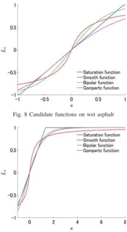
Although there is difference according to the road surface conditions, it can maybe have said that saturation function is excellent overall from simulation results. The reason is considered from the shape of each function using wet asphalt and the icy road cases.
In Fig. 8, the absolute values of gompertz function in the section of s>0.5 are smaller than the other functions. Namely, the values of gomperz function away from the top value. compared with other functions. Therefore, the effect of bringing the state close to the switching surface is weak. This
Fig. 8 Candidate functions on wet asphalt
Fig. 9 Candidate functions on icy road
makes bigger the value ofE inJ and worse the performance of slip suppression. On the other hands, smooth function has bigger value than the one of other functions at the around of s=−1 and the rate of change is big through the whole compared with others. It seems that this well-controlled change of saturation function makes goof effect to performances of driving torque and slip ratio.
From Fig. 9, we can see that the saturation function strictly reach the value of 1 rather faster than other functions. Other functions do not reach the value of 1 strictly. This means that the effect of bringing the state close to the switching surface of the other functions is rather weak than the one of saturation function. Therefore, the saturation function shows superior performance of slip suppression among all.
VI. CONCLUSION
In this paper, we present the performance analysis results of SMC with changing the chattering functions applied to slip suppression problem of EVs. The function of the following 4 was chosen as a candidate; saturation function (L0) , smooth function (L1), bipolar function (L1) and gompertz function
(L3). They are all “S-shape type” function. The performance
of SMC with each function is analyzed in slip suppression problem of EVs. Firstly, the evaluation index (J) taking into the trade-off relation in the slip suppression performance and the chattering reduction performance has been proposed for this purpose. Then, we analyze the control performance of SMC with 4 candidate functions by this index from simulations with three different road conditions, a dry asphalt
a wet asphalt and an icy road. As a result, we can see that there is no difference of 4 functions in chattering reduction performance, and that saturation function is excellent overall in slip suppression performance. Therefore, we conclude the saturation function is most suitable for slip suppression sliding mode control. In future works, it is need to extend the SMC with saturation function improving the control performance for practical use, for example, introducing the approach angle for saturation function.
ACKNOWLEDGMENTS
This research was partially supported by Grant-in-Aid for Scientific Research (C) (Grant number: 16K06409; Tohru Kawabe; 2016-2018) from the Ministry of Education, Culture, Sports, Science and Technology of Japan.
REFERENCES
[1] A. G. Mamalis, K. N. Spentzas and A. A. Mamali, The Impact of Automotive Industry and Its Supply Chain to Climate Change: Somme
Techno-economic Aspects,European Transport Research Review, Vol.5,
No.1, 2013, pp.1–10.
[2] H. Tseng and J. S. Wu and X. Liu, Affordability of Electric Vehicle for a Sustainable Transport System: An Economic and Environmental Analysis, Energy Policy, Vol.61, 2013, pp.441–447.
[3] A. T. Zanten, R. Erhardt and G. Pfaff, VDC; The Vehicle Dynamics
Control System of Bosch, Proc. Society of Automotive Engineers
International Congress and Exposition, 1995, Paper No. 950759. [4] K. Kin, O. Yano and H. Urabe, Enhancements in Vehicle Stability and
Steerability with VSA,Proc. JSME TRANSLOG 2001, 2001, pp.407–410
(in Japanese).
[5] K. Sawase, Y. Ushiroda and T. Miura, Left-Right Torque Vectoring
Technology as the Core of Super All Wheel Control (S-AWC),Mitsubishi
Motors Technical Review, No.18, 2006, pp.18–24 (in Japanese). [6] S. Kodama, L. Li and H. Hori, Skid Prevention for EVs based on the
Emulation of Torque Characteristics of Separately-wound DC Motor, Proc. The 8th IEEE International Workshop on Advanced Motion Control , VT-04-12, 2004, pp.75–80.
[7] M. Mubin, S. Ouchi, M. Anabuki and H. Hirata, Drive Control of
an Electric Vehicle by a Non-linear Controller, IEEJ Transactions on
Industry Applications, Vol.126, No.3, 2006, pp.300–308 (in Japanese). [8] K. Fujii and H. Fujimoto, Slip ratio control based on wheel control
without detection of vehicle speed for electric vehicle, IEEJ Technical
Meeting Record, VT-07-05, 2007, pp.27–32 (in Japanese).
[9] S. Li, K. Nakamura, T. Kawabe and K. Morikawa, A Sliding Mode
Control for Slip Ratio of Electric Vehicle, Proc. of SICE Annual
Conference 2012, pp.1974–1979.
[10] I. Eker and A. Akinal, Sliding Mode Control with Integral
Augmented Sliding Surface: Design and Experimental Application to
an Electromechanical system, Electrical Engineering, Vol.90, 2008,
pp.189–197.
[11] S. Li and T. Kawabe, Slip Suppression of Electric Vehicles Using Sliding
Mode Control Method,International Journal of Intelligent Control and
Automation, Vol.4, No.3, 2013, pp.327–334.
[12] V. Utkin, Variable Structure Systems with Sliding Modes, IEEE
Transactions on Automatic Control, Vol. 22, No. 2, 1977, pp. 212-222.
[13] V. Utkin,Sliding Modes and Their Applications in Variable Structure
Systems, Mir Publishers, USSR, 1978.
[14] U. M. Ch, Y. S. K. Babu and K. Amaresh, Sliding Mode Speed
Control of a DC Motor, Proc. of 2011 International Conference on
Communication Systems and Network Technologies, 2011, pp. 387-391. [15] K. Nakano, U. Sawut, K. Higuchi and Y. Okajima, Modelling and
Observer-based Sliding-mode Control of Electronic Throttle Systems, Transaction on Electrical Engineering, Electronics and Communications, Vol. 4, No. 1, 2006, pp. 22-28.
[16] Y. Li, J. O. Lee and J. Lee, Attitude Control of the Unicycle Robot Using
Fuzzy-sliding Mode Control,Proc. of the 5th International Conference
on Intelligent Robotics and Applications, Vol. 3, 2012, pp. 62-72.
[17] J. E. Slotine, W. Li, Applied Nonlinear Control, Prentice Hall, 1991,
USA.
[18] H. B. Pecejka and E. Bakker, The Magic Formula Tyre Model,Proc. of
the 1st International Colloquium on Tyre Models for Vehicle Dynamics Analysis, 1991, pp. 1-18.
[19] Y. Hori, Simulation of MFC-Based Adhesion Control of 4WD Electric
Vehicle,IEEJ Record of Industrial Measurement and Control, Vol. IIC-00,
No. 1-23, 2000, pp. 67-72 (in Japanese).