Gravity and Hydrodynamics
Masahiro Ohta
DOCTOR OF PHILOSOPHY
Department of Particle and Nuclear Physics
School of High Energy Accelerator Science
Graduate University for Advanced Studies
2012
Abstract
We study relationships between gravitational theories and hydrodynamic systems with several approaches. There are at least three approaches which realize this idea: the mem- brane paradigm, the AdS/CFT duality, the BKLS approach. In this thesis, we focus on each the AdS/CFT duality and the BKLS approach individually.
First, we examine the AdS/CFT duality and the universality of the shear viscosity to the entropy density ratio η/s for various holographic superfluids. In the study of the AdS/CFT duality, fluids corresponding to a large class of geometries ensure the universality η/s = 1/(4π). The universality has been extensively studied, and this holds for all known examples which have been studied. We study three types of the holographic superfluids as yet another example of the universality: s-wave, p-eave and (p + ip)-wave holographic superfluids. For the s-wave case, the ratio has the universal value 1/(4π) as in various holographic models. For the p-wave case, there are two shear viscosity coefficients because of the anisotropic boundary spacetime, and one coefficient has the universal value. For the other viscosity coefficient, the existing technique is not applicable since there is no tensor mode of metric perturbations which decouples from Yang-Mills perturbations. For the (p + ip)-wave case, the situation is the same as the case of the latter component in the p-wave. These results imply that p-wave and (p + ip)-wave holographic superfluids may not have the universality, and in fact, they are the first examples of the non-universal shear viscosity to the entropy density ratio.
Second, we study another realization, the BKLS approach. The BKLS approach is proposed by Bredberg et al. (1006.1902), where the fluid is defined by the Brown-York tensor on a timelike surface at r = rc in black hole backgrounds. We consider both Rindler space and the Schwarzschild-AdS (SAdS) black hole. The former describes an incompressible fluid, whereas the latter describes the vanishing bulk viscosity at arbitrary rc, but these two results do not contradict with each other. We also find an interesting “coincidence” with the black hole membrane paradigm which gives a negative bulk viscosity. In order to show these results, we rewrite the hydrodynamic stress tensor via metric perturbations using the conservation equation. The resulting expressions are suitable to compare with the Brown- York tensor.
Contents
Introduction 3
1 Hydrodynamics and Linear Response Theory 9
1.1 Linear Response Theory . . . 9
1.2 Hydrodynamics . . . 12
1.2.1 Perfect Fluid . . . 13
1.2.2 First Order Hydrodynamics . . . 14
1.2.3 Second Order Hydrodynamics . . . 16
1.2.4 Kubo Relations for the Viscosity Coefficients . . . 17
2 AdS/CFT and Hydrodynamics 19 2.1 The s-wave Superfluids . . . 21
2.1.1 Background . . . 21
2.1.2 η/s . . . 22
2.2 Anisotropic superfluids . . . 27
2.2.1 The p-wave superfluids . . . 28
2.2.2 The (p + ip)-wave superfluids . . . 30
2.3 Implications of the results . . . 32
2.3.1 Viscosity of superfluids . . . 33
2.3.2 Implication to dynamic critical phenomena . . . 35
3 Another Realization of the Relationship between Gravity and Hydrody- namics 36 3.1 Linearized hydrodynamics by Metric Perturbations . . . 36
3.1.1 Homogeneous Perturbations . . . 36
3.1.2 Inhomogeneous Perturbations . . . 39
3.2 Sound Mode in Rindler Space . . . 40
3.2.1 Thermodynamic Quantities . . . 40
3.2.2 Sound Mode Perturbations . . . 42
3.2.3 Possible Connection with the Membrane Paradigm? . . . 44
3.2.4 Inhomogeneous Perturbations . . . 45
3.3 Sound Mode in Schwarzschild-AdS Black Hole . . . 48
3.3.1 Thermodynamic Quantities . . . 48
3.3.2 Sound Mode Perturbations . . . 50
3.3.3 Homogeneous Perturbations . . . 52
3.3.4 Inhomogeneous Perturbations and Sound Pole . . . 53
3.4 Relation between Rindler and SAdS Results . . . 54
Conclusion 57 Acknowledgements 59 A Quadratic forms of perturbations for Einstein-Matter actions 60 A.1 The Quadratic Form of the Einstein-Hilbert Action . . . 60
A.2 The Quadratic Form of the s-wave Holographic Superfluid Action . . . 61
A.3 The Quadratic Form of the Einstein-Yang-Mills Action . . . 63
A.3.1 The p-wave Holographic Superfluid Action (Tensor Mode) . . . 65
A.3.2 The (p + ip)-wave Holographic Superfluid Action . . . 65
B A Note on Chapter 3 67 B.1 The Dispersion relation of Second Order Hydrodyanmics . . . 67
B.2 Several Expressions Used in Chapter 3 . . . 68
B.2.1 Integration constant . . . 68
B.2.2 Explicit expression of Eq. (3.3.14) . . . 68
Introduction
In theoretical physics, there are a large number of dualities which relate a theory to another theory. The dualities can often transform a difficult problem to an easy problem. One example of the dualities is a correspondence between (d + 1)-dimensional gravitational theories and d-dimensional hydrodynamics. There are at least three approaches which realize this duality: (i) the membrane paradigm, (ii) the AdS/CFT duality, (iii) the BKLS approach. They have been studied in different contexts. Let us explain the history of these approaches.
The oldest realization is (i) the membrane paradigm [1, 2], which has been studied in the context of the black hole physics. They tried to map the dynamics of the black hole to hydrodynamics and focused on the black hole’s event horizon. Once an object passes through the black hole’s event horizon, the object cannot affect an outside observer. In other words, the observer cannot see the inside of the black hole but can see the surface of the black hole. Therefore, the black hole dynamics should be effectively described by a dynamical membrane on the stretched horizon, a timelike surface located slightly outside the true horizon. The membrane dynamics is described by the Einstein equation on the stretched horizon and the equation is the same as the Navier-Stokes equations, mathematically. However, the membrane paradigm has the unpleasant features as a fluid such as a negative bulk viscosity. In addition, the microscopic realization of the membrane paradigm is not clear.
On the other hand, (ii) the AdS/CFT duality [3, 4, 5, 6], based on string theory, provides several explicit realizations of microscopic understandings of the corresponding hydrody- namics since the D-branes[7] provide both the asymptotic AdS black brane geometries and the corresponding strongly coupled field theories, which live on the boundary of the AdS geometries. For example, the D3-branes provides the AdS5×S5 geometry and the strongly coupledN = 4 Super Yang-Mills theory in the large-Nc limit. One of the most important features of the AdS/CFT duality is that exact correlation functions of the strongly coupled field theories can be derived from the classical gravity, which is easy to calculate.
Therefore, the AdS/CFT duality has been applied to real-world physics e.g., the quark-
gluon plasma. The quark-gluon plasma can be described as a strongly coupled viscous fluid according to the heavy-ion collision at RHIC. Using the AdS/CFT duality, it turned out that the strongly coupledN = 4 Super Yang-Mills theory and the quark-gluon plasma have almost same value of the shear viscosity to the entropy density ratio η/s. It may sound strange at the first glance since they are quite different field theories. But the agreement of the η/s would be because of the universality of the strong coupled field theories. (See the next section for more detail on the universality.) Therefore, it is important to find such robust and universal features to apply the AdS/CFT duality to real-world physics. More recently, the AdS/CFT duality has been applied to the condensed matter physics. The condensed matter physics is a low energy effective theory, so it is important to find the IR fixed point. This idea is realized by the holographic renormalization group that the field theory lives on arbitrary timelike surface, and the position of the surface corresponds to the energy scale of the field theory. The boundary and the horizon of the geometry correspond to the UV limit and the IR limit of the field theory, respectively. Therefore, the dependence on the position of the timelike surface is interpreted as the Wilsonian renormalization group flow of the field theory.
The UV limit of the field theory should be a conformal field theory as long as the cor- responding geometry is asymptotic AdS. However, real world materials are not confromally invariant in the UV limit. In the context of the Wilsonian renormalization group, the renor- malized field theory doesn’t depend on the physics above the cutoff scale. So, (iii) Bredberg, Keeler, Lysov, and Strominger proposed an approach which doesn’t depend on the asymp- totics of the geometry [27, 28]. They introduced a timelike surface at arbitrary position for the “boundary” where the fluid lives. This approach doesn’t provide microscopic under- standing of the fluid but should describe robust features of the correspondence between the gravity and hydrodynamics, instead.
In this thesis, we focus on each (ii) the AdS/CFT duality and (iii) the BKLS approach, and study the relationship between them.
The AdS/CFT duality (Chapter 2)
In the context of the relationship between gravitational theories and hydrodynamics, the shear viscosity, one of the transport coefficient, has been extensively studied. This is because η/s, the ratio of the shear viscosity to the entropy density, is universal, i.e.,
η s =
1 4π ,
according to the AdS/CFT duality, the membrane paradigm and the BKLS approach. Es- pecially, in the context of AdS/CFT, the universality has been extensively studied, and this holds for all known examples which have been studied (See, e.g., Ref. [8, 9]).
The shear viscosity to the entropy density ratio η/s was first derived for the D3-brane [10], which is the dual of N = 4 SYM. Then the same results were obtained for the M2- and M5-branes [11]. These three branes are the duals of conformal theories. Moreover, the universality holds even if theories are non-conformal, e.g., Dp-branes for p 6= 3, the Klebanov-Tseytlin geometry, the Maldacena-Nunez geometry, and the N = 2∗ system [12, 13, 14, 15, 16]. For the application to real QCD, each the finite density theories [17, 18, 19, 20] and the theories with fundamental fermions has been studied [21]. They are the duals of the charged black holes and the D3-D7 system, respectively. They ensure the universality. Even for a time-depending systems, the universality is held [22]. For the application to condensed matter physics, the Lifshitz-like geometry have the universality [23] Although there exists several arguments to generally support the universality [24, 25], it is still unclear why the universality holds microscopically and how generic the universality is.
In this Thesis, first, we study the holographic superfluids, which provide yet another example of the universality. The holographic superfluids exhibit a second-order phase tran- sition. We study three types of the holographic superfluids, s-wave, p-wave, and (p + ip)- wave. They are characterized by the order parameter of the phase transition, i.e., in the bulk gravitational theories, the order parameter of the s-wave holographic superfluids is a scalar field, and the one of both p-wave and (p + ip)-wave holographic superfluids is a SU(2) gauge field. (The difference between the p-wave and (p + ip)-wave is condensing compo- nents of the gauge field.) We found following results: (i) the s-wave holographic superfluids holds the universality of η/s, (ii) the p-wave and (p + ip)-wave holographic superfluids may have non-universal η/s because of the spacial anisotropy coming from the gauge field. (We will discuss the relationship between the universality violation and the spacial anisotropy in Sec. 2.2.) These are the first examples of the non-universal system. Actually, our work triggered detailed studies of the non-universal shear viscosity [86, 87, 88, 89].
The BKLS approach (Chapter 3)
Let us summarize the three approaches again in order to realize the feature of the BKLS approach.
1. Historically, the membrane paradigm [1, 2] is the oldest one. In this case, the fluid lives on the stretched horizon r→ r0. However, the membrane paradigm has the unpleasant features as a fluid such as a negative bulk viscosity. The membrane paradigm originally
focuses on the (3 + 1)-dimensional asymptotically flat black holes, but asymptotics should not matter much since it focuses on the near-horizon limit.
2. In the AdS/CFT duality, the dual fluid “lives” at the AdS boundary r → ∞. The advantage of the AdS/CFT duality is a clear microscopic interpretation for the dual fluid. The AdS/CFT results are widely used for real-world applications such as the quark-gluon plasma. (See, e.g., Refs. [8, 9, 26] for reviews.)
3. More recently, Bredberg, Keeler, Lysov, and Strominger (BKLS) [27, 28] proposed the timelike surface at arbitrary position r = rc for the “boundary” where the fluid lives (See also, e.g., Refs. [29, 30]). The BKLS approach is analogous to the holo- graphic renormalization. In the near-horizon limit, the BKLS approach describes an incompressible fluid.
Another closely related idea is a “black hole in a cavity” [31]. This idea was proposed to obtain a well-defined thermal equilibrium for asymptotically flat black holes such as the Schwarzschild black hole. The Schwarzschild black hole has a negative heat capacity, so it is unstable by the Hawking radiation. However, if the black hole is surrounded by a finite- temperature cavity, and if the cavity is close enough to the horizon, a thermal equilibrium is achieved. In a sense, the BKLS approach is an AdS black hole in a cavity.
While each approach has a different motivation and physical interpretation, one thing is common: they all employ the Brown-York tensor [32] as the fluid stress tensor. Thus, they are somehow related to each other.
Both in the membrane paradigm and in the BKLS approach (in particular in Ref. [28]), one often starts to identify the velocity field of the fluid in the bulk spacetime. This has its own advantage that the relationship between the Einstein equation and the Navier-Stokes equation is direct and transparent. On the other hand, this brings us an immediate problem why a particular vector field should be regarded as the velocity field. So, we do not take such a path.
• Instead, we consider metric perturbations and study the (linear) response of the Brown-York tensor by the perturbations `a la AdS/CFT duality.
• In hydrodynamics, the velocity field is determined from the metric perturbations (Sec. 3.1). Then, one can eliminate the velocity field completely in the hydrodynamic stress tensor. The resulting expression contains metric perturbations only, which is suitable to compare with the Brown-York tensor. In our approach, the velocity field is a consequence of metric perturbations.
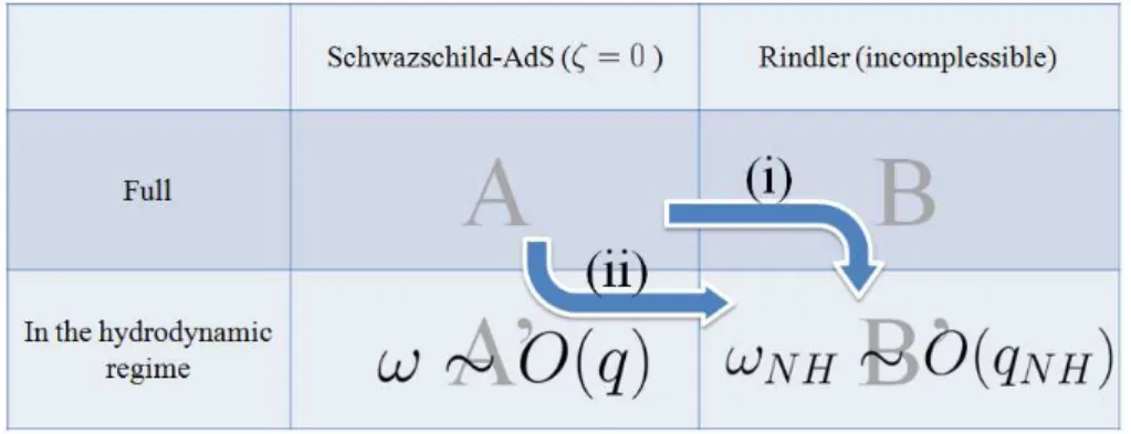
One purpose of this chapter is to reexamine the BKLS approach using the above formulation. In particular, we study the issue of the bulk viscosity ζ, which is non-negative in the AdS/CFT duality, negative in the membrane paradigm, and is irrelevant in the BKLS approach (because of an incompressible fluid). For that purpose, we consider the sound mode perturbations whose analysis was somewhat incomplete in Ref. [27]. We study Rindler space, which is the near-horizon limit of black holes with nondegenerate horizon, and the five-dimensional Schwarzschild-AdS black hole (SAdS5)1. Our results are summarized as follows:
1. For Rindler space, the Brown-York tensor gives an incompressible fluid in accordance with the BKLS result (Sec. 3.2).
2. For the SAdS5 black hole, the Brown-York tensor always gives the vanishing bulk viscosity irrespective of the boundary position rc (Sec. 3.3).
3. There are no contradictions between two results since the hydrodynamic regime used for the SAdS black hole “differs” from the hydrodynamic regime used for Rindler space (when expressed in terms of the SAdS variables) (Sec. 3.4).
In addition, we obtain one of the second-order hydrodynamic transport coefficient τπ for the SAdS5 black hole in the BKLS approach.
The framework of this thesis
This thesis is organized as follows. In Chapter 1 we shall give a short review of the linear response theory, which provides the response of an operator induced by small perturbations on the thermal equilibrium. It is necessary in order to obtain the transport coefficients from perturbations. We shall review the basics of the hydrodynamics, which include the isotropic first order hydrodynamics and the second order hydrodynamics.The anisotropic fluid is dual to the p-wave and (p + ip)-wave holographic superfluids. In the context of the AdS/CFT duality, the corresponding fluid usually has the conformal symmetry. The SAdS black hole with a finite cutoff, however, might not have conformal symmetry. So the non-conformal second order fluid should be considered. Using the linear response theory and the hydrodynamic constitutive equation, we will find the response of the hydrodynamic stress tensor induced by the gravitational perturbations, and the viscosities finally.
1While our work was in progress, there appeared preprints which study Rindler hydrodynamics [33, 34, 35].
Chapter 2 contains a brief review of AdS/CFT and the study of the ratio η/s of the holo- graphic superfluid, simultaneously. First, we shall show the s-wave holographic superfluids have a universal shear viscosity. This proof includes a large class of geometries and is the most general theorem of the universality at present. Then we discuss anisotropic viscosities of the p-wave and (p + ip)-wave holographic superfluids and they can have non-universal value. The study is based on our paper [36].
In Chapter 3, which is based on our research [37], we shall present another realization, the BKLS approach. We define the approach in terms of the Brown-York tensor and metric perturbations. First, we write down the linear response of the hydrodynamic stress tensor in terms of the metric perturbations. Then we show the linear perturbation of the Brown- York tensor in the Rindler space. Comparing the Brown-York tensor and the hydrodynamics stress tensor, we shall reproduce the results of the BKLS approach. In order to compare with the SAdS5 black hole, we shall derive the viscosities, especially the bulk viscosity, of SAdS5 with arbitrary rc and show that the bulk viscosity vanishes even for arbitrary rc. We shall discuss how they can be compatible. We also compute a second-order hydrodynamic coefficient τπ for arbitrary rc.
Chapter 1
Hydrodynamics and Linear Response
Theory
Here, the minimal formalism of hydrodynamics and the linear response theory are ex- plained.
1.1 Linear Response Theory
Linear response theory is based on the following conditions:
• Hamiltonian in the system can be decomposed into the time independent part and the time depending part.
• The time depending part is made of a small fluctuation which is perturbed from the outside of the system.
• The system was thermal equilibrium in the past.
The time depending density of state ρ(t) and time depending Hamiltonian H(t) satisfies the von-Neumann equation
i∂
∂tρ(t) = [H(t), ρ(t)] . (1.1.1)
This means the time evolution of the density of state is
ρ(t) = U (t, t0)ρ(t0)U†(t, t0) . (1.1.2)
Even if the system depends on time, the expectation value of an arbitrary observable B at time t can be represented by
hBit= T rρ(t)B . (1.1.3)
It is, however, difficult to calculate the time depending expectation value exactly. So we take the most simple assumption that the system was in thermal equilibrium and then perturbed linearly.
First, we take Schr¨odinger picture. Assume that H(t) can be decomposed into the time independent part H0 and the time dependent part δH(t), and the time dependent part is made of the time independent operator OA(x) and its time dependent source φA(t, x):
H(t) = H0+ δH(t), δH(t) =− Z
dxd−1φA(t, x)OA(x) . (1.1.4) The time evolution operator from t0 to t satisfies the following differential equation.
i∂
∂tU (t, t0) = H(t)U (t, t0), U (t0, t0) = 1 . (1.1.5) The solution is
U (t, t0) = T
· exp
µ
−i Z t
t0
dsH(s)
¶¸
. (1.1.6)
This time evolution operator also should be decomposed into the H0 part and the δH(t) part. First, the H0 part can be clearly defined as
U0(t, t0) = exp (−i(t − t0)H0) . (1.1.7) Then we naively define the δH(t) part as1
U (t, t0) = U0(t, t0)Ui(t) . (1.1.8) This definition and the time evolution equation for the full Hamiltonian lead the time evolution equation for δH(t) .
id
dtUi(t) = U
†
0(t, t0)δH(t)U0(t, t0)Ui(t)
= δHI(t)Ui(t) .
(1.1.9)
1The subscript “i” in Ui means “Interaction part”. Don’t confuse this with the subscript “I”, which means “Interaction pictuer”.
Here, the time dependent part of the Hamiltonian in the interaction picture is defiened as δHI(t) := U0†(t, t0)δH(t)U0(t, t0) . (1.1.10) Note that the time evolution of states is under Ui and of operators is under U0 in the interaction picture. The solution of Ui(t) is
Ui(t) = T
· exp
µ
−i Z t
t0
dsδHI(s)
¶¸
. (1.1.11)
So the naive definition reads the proper expression eventually. Now using the expansion of the full time evolution operator
U (t, t0) = U0(t, t0) µ
1− i Z t
t0
dsδHI(s) +O(δHI2)
¶
, (1.1.12)
one can derive the first order approximation of the expectation value of the arbitrary ob- servable B
hBit= T rU (t, t0)ρ(t0)U†(t, t0)B
= T rρ(t0)BI(t, t0) + i Z t
t0
dt1T rρ(t0)[δHI(t1), BI(t, t0)] +O(δHI2) . (1.1.13)
Let the system be thermal equilibrium at t0 so δHI(t0) = 0 and the density of state becomes
ρ(t0) = e
−βH0
T re−βH0 =: ρ0 . (1.1.14)
Therefore, the state density commute with U0(t, t0) and so T rρ(t0)BI(t, t0) = T rρ0B. The first order approximation become
hBit= T rρ0B + i Z t
t0
dt1T rρ0[δHI(t1), BI(t, t0)] +O(δHI2) . (1.1.15)
If we take the arbitrary observable B = OA(x), the response of the expectation value can be written as
δhOAi(t, x) = i Z t
t0
dt1
Z
dd−1x′T rρ0[OIA(t, x),OIB(t′, x′)]φB(t′x′)
= i Z ∞
−∞
dt′ Z
dd−1x′θ(t− t′)h[OIA(t, x),OIB(t′, x′)]iφB(t′x′) ,
(1.1.16)
UsingR dd−1xdteiωt−ikx to transform it into the Fourier space expression,
δh ˜OAi(ω, k) = −GRAB(ω, k) ˜φB(ω, k) , (1.1.17)
where we defined the Retarded Green’s function GRAB(ω, k) = −i
Z ∞
−∞
ddxeiωt−ikxθ(t)h[OA(t, x),OB(0, 0)]i . (1.1.18)
This expression means that even if the system depends on time, the first order approximation in the fluctuation can be understood in terms of the information of thermal equilibrium quantities.
1.2 Hydrodynamics
The hydrodynamics is an effective theory under long wave length limit, i.e., the derivative expansion. The referential scale in the hydrodynamics is the mean free path ℓ. Therefore, the validity of the hydrodynamic approximation is controlled by the combination of the characteristic momentum scale and the mean free path (k· ℓ).
One of the most distinctive features of hydrodynamics is that it is based on the con- servation equations and the constitutive equation for the hydrodynamic stress tensor, not certain Lagrangian. The reason why the constitutive equation should be introduced is that the differential equations from the conservation equations is not closed themselves. The constitutive equation for the hydrodynamic stress tensor reduces the degrees of freedom and then the differential equations can be closed.
The constitutive equation is constructed by the derivative expansion. So the hydrody- namic stress tensor of the perfect fluid does not include any derivatives.
Tµν = Tperfectµν +O(∂1) . (1.2.1)
If (k· ℓ) is small enough to be neglected, the system can be described by the perfect fluid. Since the hydrodynamics is an effective theory, each fluid is characterized by several coefficients, which is called transport coefficients. The number of the transport coefficients can be determined by the symmetry of each system. For example, the isotropic fluid has the two first order transport coefficients η and ζ. This is because the symmetric rank two tensor transforming under SO(d− 1) can be decomposed into the two irreducible representations, which are the symmetric traceless part and the trace part. Therefore, to fix the transport
coefficient in a hydrodynamic system is to fix the equation of motion in the hydrodynamic system.
In this section, we construct the constitutive equations for several fluids, derive Kubo formula for the first order transport coefficients and find the dispersion relations using the equation of motions in an arbitrary curved background. Following discussion is based on [38] and [9] for the first order fluids, and [39] for the second order fluids. (See [40, 41, 42, 43] for more detail on the second order hydrodynamics.) Note that the readers should mind that, in this section, we discuss the boundary theory from the point of view of AdS/CFT although we discuss the fluid on the curved spacetime.
1.2.1 Perfect Fluid
The equation of motion of the hydrodynamics is based on the conservation equation.
∇µTµν = 0 , (1.2.2)
where Tµν is the hydrodynamic stress tensor of the fluid. Here, we impose that the system is locally equilibrium: the system is thermal equilibrium in the neighborhood of an arbitrary position x. So the thermodynamic quantities can be defined there and the state of the neighborhood can be specified by the thermodynamic quantities and the fluid velocity uµ, which is normalized as uµuµ = −1. This means that the constitutive equation is Tµν = Tµν(uµ, P,· · · ), where P is the pressure of the system. They are locally defined.
Now we derive the constitutive equation of the perfect fluid. Let the dimension of the spacetime d-dimension. Consider an infinitesimal volume element and its surface element dΣµ. The momentum flux through the µ surface is
dqi = TiνdΣν . (1.2.3)
Especially in the rest flame, the volume element doesn’t carry total momentum, so Ti0 = 0 and the pressure against each surface is same and perpendicular since the volume element doesn’t move. In addition, this volume element is not affected by the next volume element since the dissipative momentum transfer is not exist. Therefore,
Tij = P δij . (1.2.4)
The energy density in the volume element is T00= ǫ, so the generally covariant form of the
hydrodynamic stress tensor is
Tµν = ǫuµuν + PµνP , (1.2.5)
where Pµν is the projection operator defined by
Pµν = uµuν + gµν . (1.2.6)
One can show that the fluid described by (1.2.5) doesn’t have dissipation, using the thermodynamic relations. Projecting the divergence of the hydrodynamic stress tensor along uµ
0 = uν∇µ(wuµuν + P gµν)
=−T ∇µ(σuµ) , (1.2.7)
where we introduced the enthalpy w = ǫ + P and the entropy density σ, and we used the thermodynamic equation dw = T dσ + dp and ǫ + P = T σ. The entropy flux is conserved.
∇µ(σuµ) = 0 . (1.2.8)
This means the system represented by the hydrodynamic stress tensor (1.2.5) does not have any dissipation.
1.2.2 First Order Hydrodynamics
In order to pick up the effect of the dissipation, we examine the derivative term τµν. Tµν = (ǫ + P )uµuν + P gµν− τµν . (1.2.9) Let us consider τµν up to the first derivative in the isotropic system. This approximation is valid when (k· ℓ)2 ≪ 1. Now we should reconsider the definition of the fluid velocity. We define the velocity in the condition that, in the rest flame of any given volume element, the momentum of the volume element is zero and its energy is expressed in terms of the same formulae as when dissipative processes are absent. This means that τµνuν = 0 and, in the rest flame, the spatial direction of the fluid velocity is absent ui = 0. Therefore, in the proper coordinate only τij should be exist.
Decomposing τij into the irreducible representations of SO(d− 1),
τij = η µ
∂iuj+ ∂jui−
2 pδij∂ku
k
¶
+ ζδij∂kuk , (1.2.10)
where ζ is the bulk viscosity and η is the shear viscosity, and p denotes the spatial dimension d−1. Since the bulk viscosity is the trace part of the hydrodynamic stress tensor, it provides the force which change the volume of the element. In the conformal fluid, the bulk viscosity is absent since its hydrodynamic stress tensor is traceless. On the other hand, the shear viscosity provides the force which change the shape of the volume element without its volume unchanging. In the general covariant form,
τµν = PµαPνβ
· η
µ
∇αuβ+∇βuα− 2
pgαβ∇γu
γ
¶
+ ζgαβ∂γuγ
¸
. (1.2.11)
Note that the projection operator is introduced in order to preserve the condition τµνuν=0. The positivity of the entropy production restricts the transport coefficients. As the perfect fluid, the time component of the conservation equation in the proper coordinate (∇µTµν)uν = 0 leads
∇µ(σuµ) = 1 T
µ
τ<µν>u<µν>+ 1 pPαβτ
αβPµνu µν
¶
. (1.2.12)
Here, the spacially projected symmetric traceless symbol A<µν> := 1
2P
µαPνβ(A
αβ+ Aβα)−1 pP
µνPαβA
αβ , (1.2.13)
and the symmetrized first derivative of fluid velocity uµν := 1
2(∇µuν +∇νuµ) , (1.2.14) are defined. Eq. (1.2.12) means that, in order to keep the entropy production positive for any given velocity, the symmetric traceless part of the viscous tensor τ<µν> and trace part of that Pµντµν must proportional to u<µν> and Pµνuµν, respectively. In addition, the coefficient of each term must positive. Therefore, the transport coefficients η and ζ should be positive.
Since the equation of motion is closed, one can derive the poles of the linearized hydro- dynamics. We derive them in Sec. 3.1.
1.2.3 Second Order Hydrodynamics
We proceed the derivative expansion of the hydrodynamic stress tensor up to second order. Therefore, the viscous tensor τµν in eqviscousstresstensor must include all possible second-order terms2.
Basically, the second order hydrodynamics should be introduced when the characteristic momentum scale of the system compared with the mean free path, i.e., (k · ℓ)2, cannot be neglected. There is another understanding to introduce the second order term. In the first order “relativistic” hydrodynamics, the speed of propagation for heat and viscosity are infinite since the EOMs for the propagation obey parabolic differential equation, which is the same as the traditional thermal diffusion equation. Eventually, the first order “relativistic” hydrodynamics is only applicable to the system slowly varying on space and time scales characterized by the mean free path ℓ and the momentum k. Israel introduced the second order derivative terms because of the latter motivation [40], and then he generalized the theory in the curved background [41]. (See appendix of Ref.[42] for review.)
From the AdS/CFT duality’s point of view, conformal symmetry is so important, so the second order hydrodynamics with conformal invariance is required. Baier et al. constructed the theory and found additional terms [39] which were neglected in Refs.[40, 41]3. Then the most general isotropic second order hydrodynamics without charges are constructed [43].
In this thesis, we don’t need the non-linear terms. So we introduce a non-conformal viscous tensor:
τµν =− ησµν − ζ(∇ · u)Pµν
+ ητπ<∇uσµν>+ ζτΠ∇u(∇ · u)Pµν + κ1Rα<µν>βu
αuβ+ κ2R<µν>+¡κ3Rαβuαuβ+ κ4R¢ Pµν ,
(1.2.15)
where the antisymmetric traceless tensor σµν is defined by σµν := 2<∇µuν>. We have introduced six second order coefficients, i.e., τπ, τΠ, κ1, κ2, κ3, κ4. Note that, for the conformal fluids, τΠ, κ3 and κ4 are absent, and κ1 =−(d − 2)κ2. (cf. Ref.[39].)
2In this thesis, we consider only the isotropic second order hydrodynamics.
3There are two types of the additional terms. First, Baier et al. found the terms made of Riemann tensor and Ricci tensor. Second, in order to preserve conformal invariance, additional non-linear terms are required.
1.2.4 Kubo Relations for the Viscosity Coefficients
The viscosity coefficients represent the dissipation of the fluid, so they can be obtained by linear response theory. Linear response theory is based on the operator of interest and its corresponding source. Since we are now interested in the response of the hydrodynamic stress tensor Tµν, the appropriate source is the metric gµν.
In order to apply linear response theory to the viscous hydrodynamics, the state where the spacial component of the velocity is absent uµ = (1, 0, 0,· · · , 0) and the spacetime is perturbed by the spatially homogeneous metric perturbation around the flat spacetime ηµν4, gij = δij+ hij(t), hij ≪ 1, hii= 0 (1.2.16)
g00 = −1, g0i(t, x) = 0 . (1.2.17)
The response of the velocity δuµ from the metric perturbation is absent since the homoge- neous perturbation preserve the spatial rotational isometry and one can show the normal- ization uµuµ=−1 preserve δu0 = 0.
The response of the energy momentum tensor is
δTij = P hij + η∂0hij, (i6= j) . (1.2.18) Using (1.1.17), one can find the Green’s function of the off-diagonal hydrodynamic stress tensor,
G12,12R (ω, 0) =−i Z ∞
−∞
ddxeiωtθ(t)h[T12(t, x), T12(0, 0)]i = −iηω + O(ω2) . (1.2.19)
Here, we took i = 1, j = 2 without loss of generality because of the SO(p) spatial isometry. The first term is called contact term, which is independent of the frequency. Removing the contact term by hand, one can obtain the shear viscosity from the Green’s function.
η =− lim
ω→0
1 ωImG
12,12
R (ω, 0) . (1.2.20)
This is the Kubo relation for the shear viscosity.
We use Eq. (1.2.20) in Chapter 2. Although there are several Kubo relations for the other viscosities, we don’t discuss them here. We discuss the response of the hydrodynamic
4The homogeneous perturbation correspond to the long wave length limit k→ 0. In general, we should take care of the order of the limit. Sometimes, the limit and another limit are non-commutative.
stress tensor from the sound mode metric perturbation in Sec. 3.1.
Chapter 2
AdS/CFT and Hydrodynamics
Historically, AdS/CFT is proposed by Maldacena[3] in 1997. He proposed that the strong coupling and the large Nc-limit of theN = 4 super Yang-Mills theory, which is the low energy effective theory of D3-brane, corresponds to the near horizon limit of the black D3-brane solution. And then Gubser, Klebanov, and Polyakov[6], and Witten[4] proposed the prescription for obtaining the correlation function of operators in the field field theory from the calculus in the corresponding bulk gravitational theory. The prescription is called GKP-Witten relation.
Although they formulate the relation in Euclidean signature, in order to find time depen- dent dynamics, especially dynamics with dissipation, the real time formalism is needed. Son and Starinets found the prescription to obtain Retarded Green’s functions exactly in real time Lorentzian signature[44], and they derived the shear viscosity to the entropy density ratio forN = 4 super Yang-Mills (SYM) plasma[10, 45]. The ratio has been studied widely in order to understand real quark gluon plasma (QGP).
The prescription enables us to find the dissipative dynamics in the boundary theory through retarded Green’s functions. It is interesting to study the dissipative dynamics in not only QGP but condensed matter physics as well. In this thesis, we focus on the holographic superfluids, which exhibit the second order phase transition and superfluid-like behaviors.
In the studies of holographic superfluids [47, 48, 49, 50, 51, 52, 53] (See, e.g., Refs. [54, 55, 56] for reviews), one often uses numerical computations or some approximations. This is because the holographic superfluids are Einstein-matter systems and it is in general difficult to solve such systems. One approximation often employed is the “probe approximation,” where the backreaction of matter fields onto the geometry can be ignored. While the approximation is enough to see the phase transition and to compute properties such as
the conductivity, gravitational properties of these systems, in particular analytic results are largely intact. It is desirable to obtain gravitational properties of these systems analytically. We investigate this issue in this thesis. We study η/s, the ratio of the shear viscosity to the entropy density for holographic superfluids.
Technically, the universality largely depends on the following two properties of the bulk theory:
1. One can use the Kubo formula to compute η and carry out the tensor mode compu- tation of gravitational perturbations. There are no other fields which transform as a tensor even if matter fields are present.
2. The entropy density is given by the Bekenstein-Hawking formula as long as the grav- itational action takes the Einstein-Hilbert form.
In this thesis, we consider three class of holographic superfluids, the s-wave, p-wave, and (p + ip)-wave holographic superfluids in (d + 1)-dimensional bulk spacetime. Our results are summarized as follows:
(i) The s-wave holographic superfluids are described by Einstein-Maxwell-complex scalar systems [47, 48, 51]. In this case, the universality holds with a modification of the technique in Ref. [25].
(ii) The p-wave holographic superfluids are described by Einstein-Yang-Mills systems [49]. In this case, the Yang-Mills field breaks the SO(d− 1) rotational invariance on the boundary theory, which has two implications. First, the hydrodynamic limit is not described by a single shear viscosity.1 Second, for d = 3, one does not have a tensor mode which decouples from the Yang-Mills field. (Namely, item 1 of the above list fails.) As a result, the existing technique is not applicable. However, for d ≥ 4, one has the SO(d− 2) invariance. In this case, a tensor mode exists, and the universality holds for the shear viscosity associated with the tensor mode.
(iii) The (p+ip)-wave holographic superfluid is described by the same system as the p-wave holographic superfluid (with d = 3), but the symmetry breaking pattern is different [50]. Although the metric keeps the SO(2) invariance, the Yang-Mills field breaks the SO(2) invariance. As a result, there does not exist the tensor mode which decouples from Yang-Mills perturbations and the existing technique is not applicable.
1In the context of the AdS/CFT duality, anisotropic shear viscosities have been computed for the non- commutativeN = 4 plasma [57].
Our results indicate that the shear viscosity has no singular behavior across the phase transition for holographic superfluids (See Sec. 2.3.2).
The plan of this chapter is as follows. In Sec. 2.1, we consider η/s for the s-wave holographic superfluids, explaining basic prescriptions of AdS/CFT. In Sec. 2.2, we consider anisotropic holographic superfluids, the p-wave and (p + ip)-wave holographic superfluids. For the (p + ip)-wave case, we identify the Yang-Mills perturbations which couple to the would-be tensor mode of metric perturbations.
2.1 The s-wave Superfluids
2.1.1 Background
The s-wave holographic superfluids are described by Einstein-Maxwell-complex scalar system:
Ss = 1 16πGd+1
Z
dd+1x√−g
½
R− 2Λ − 1
4K1¡|Ψ|
2¢ FM NF M N
− K2¡|Ψ|2¢ |∇MΨ− iqAMΨ|2− V ¡|Ψ|2¢
¾ (2.1.1)
with the ansatz
ds2d+1 = −gtt(r)dt2+ gxx(r)
d−1
X
i=1
dx2i + grr(r)dr2 , (2.1.2)
A = At(r)dt , (2.1.3)
Ψ = Ψ(r) . (2.1.4)
Here, capital Latin indices M, N, . . . run through bulk spacetime coordinates (t, xi, r), where (t, xi) are the boundary coordinates and r is the AdS radial coordinate. Greek indices µ, ν, . . . run though only the boundary coordinates. K1, K2 and V are arbitrary real func- tions of the scalar field. This action includes not only the conventional s-wave holographic superfluids [47, 48] but also generalized models [58, 59, 60]. We impose the regularity condition on the metric at the horizon r = rh:
gtt→ ct(r− rh) , gxx → cx , grr → cr(r− rh)−1 . (2.1.5)
These conditions fix the Hawking temperature and the entropy density of the bulk geometry:
T = 1 4π
r ct
cr
, s = c
(d−1)/2 x
4Gd+1
. (2.1.6)
The model exhibits a second-order phase transition. At high temperatures, the scalar field Ψ vanishes and one obtains the standard Reissner-Nordstr¨om-AdS black hole. But at low temperatures, the Reissner-Nordstr¨om-AdS black hole becomes unstable and is replaced by a charged black hole with a scalar “hair.”
This system is supposed to be dual to some kind of superconductors/superfluids. In fact, the low temperature phase shows the expected behavior for superconductors/superfluids. As superconductors, one can see the divergence of the DC conductivity, an energy gap proportional to the size of the condensate, and the holographic London equation [48, 51, 61, 62]. As superfluids, one can see the existence of the second and fourth sounds [63, 64]. Also, vortex solutions have been constructed [65, 66, 67, 68, 69].
2.1.2 η/s
Since we are interested in the viscosity, the main object to study is the boundary energy- momentum tensor. According to the standard AdS/CFT dictionary [3, 4, 5, 6], the bulk gravitational perturbations act as the source for the boundary energy-momentum tensor. Thus, our task amounts to solve the bulk gravitational perturbations.
Consider the fluctuations of the energy-momentum tensor Tµν which behaves as e−iωt. The fluctuations are decomposed by the little group SO(d−1) acting on xi(i = 1,· · · , d−1). The fluctuations are decomposed as the tensor mode, the vector mode (“shear mode”), and the scalar mode (“sound mode”).
One can use various methods to compute the shear viscosity. Among them, the most powerful one is the Kubo formula method , which uses the tensor mode (1.2.20) :
η =− lim
ω→0
1 ωIm G
1212R (ω,~0) , (2.1.7)
where G1212R (ω,~0) is the retarded Green function for the tensor mode T12 at zero spatial momentum (1.2.19):
G1212R (ω,~0) =−i Z ∞
−∞
ddx eiωtθ(t)D[T12(t, ~x), T12(0,~0)]E . (2.1.8)
To obtain the retarded Green function, we consider homogeneous gravitational pertur-
bations which take the form
gM N = ¯gM N + hM N , (2.1.9)
where ¯gM N is the background metric (2.1.2). In the Lorentzian prescription of the AdS/CFT duality [44], the retarded Green function (2.1.8) can be calculated from the tensor mode h12. We expand the action in terms of φ(t, r) := h12(t, r) up to quadratic order and use the Fourier transformation
φ(t, r) =
Z ddk (2π)de
−iωt+i~k·~xf
k(r) ˜φ0(k). (2.1.10) The retarded Green function is obtained as follows:
1. Solve the classical equation of motion for the field fk(r) with the ingoing-wave bound- ary condition at the horizon and fk(r)→ 1 at the boundary.
2. Substitute the classical solution into the action and represent the action in terms of the boundary value ˜φ0. Only surface terms remain, and drop the contribution from the horizon.
3. The retarded Green’s function is given by the kernel of the on-shell action:
Son-shell =−1 2
Z ddk
(2π)dφ˜0(−k)GR(k) ˜φ0(k) (2.1.11) where the on-shell action is defined as Son-shell = (S + SGH+ Sc.t.)|on-shell. SGH is the Gibbons-Hawking term to provide a correct variational problem for the background geometry. Sc.t. is the counterterm to renormalize divergences in the classical action. Thus, the problem is to solve the equation of motion for the field φ under the appropriate boundary conditions.
From Eq. (2.1.1), the action which is quadratic in φ is
(2)S
s = 1
16πGd+1
Z
dd+1x
"
−1 2
√¯g(∇Mφ)2
+ ∂r
½√
¯ g
µ
2grrφ∂rφ + 1 2
g′xx gxx
grrφ2
¶¾# ,
(2.1.12)
with the help of background equation of motions (See Appendix A.2). Because of the little group SO(d− 1) acting on xi, the tensor mode of the metric perturbations decouples from
the rest of perturbations: the other modes of the metric perturbations hM N, the gauge field perturbations δAM and the scalar field perturbation δΨ. Thus, they can be set to zero consistently. Since the background geometry must satisfy the stationary condition, we add the Gibbons-Hawking term
SGH = 1 16πGd+1
Z
r→∞
ddx√−γ2K , (2.1.13)
where γµν is the boundary induced metric, nM is the normal vector to the boundary and K = γµν∇µnν is the trace of the extrinsic curvature of the boundary. This provides surface terms
(2)S
GH = 1
16πGd+1
Z
r→∞
ddx µ
−2√gg¯ rrφ∂rφ− √1g
rr
∂r¡√−¯γ¢ φ2
¶
. (2.1.14)
Therefore, the bare action is
(2)(S
s+ SGH) = 1 16πGd+1
Z
dd+1x√¯g
·
−12(∇Mφ)2
¸
+ 1
16πGd+1 Z
r→∞
ddxµ g
xx′
2gxx
√−¯γ
√g
rr −
√1g
rr
∂r¡√−¯γ
¢
¶ φ2 .
(2.1.15)
The action diverges as r → ∞, so the counterterms at the boundary must be added. We need only the gravitational counterterm in order to evaluate the retarded Green’s function for the energy-momentum tensor. According to the holographic renormalization procedure, the counterterm is
Sc.t.=− 1 16πGd+1
Z
r→∞
ddx√−γ· 2(d− 1)
L +
L
d− 2R[γ]
+ L
3
(d− 4)(d − 2)2 µ
Rµν[γ]Rµν[γ]− d
4(d− 1)R[γ]
2
¶ +· · ·
¸ ,
(2.1.16)
where L is the AdS radius andRµν[γ] is the Ricci tensor made from the induced metric γµν. These terms largely depend on the spacetime dimensions2. However, in order to evaluate the shear viscosity, we need boundary terms only up to first order in ω: O(ω2) terms in the action do not contribute to the Kubo formula because of the ω→ 0 limit. So, only the first
2One has to be careful when the number of the boundary spacetime dimensions d is an even number. See Ref. [70] for details.
term in Eq. (2.1.16) is important and it becomes
(2)S
c.t. = 1 16πGd+1
Z
r→∞
ddx√−¯γ(d − 1)φ2 , (2.1.17)
for the tensor mode perturbation. This term removes the divergences from the second term of Eq. (2.1.15). As a result, the renormalized action is
16πGd+1(2)(Ss+ SGH+ Sc.t.)
=
Z ddk
(2π)dφ˜0(−k) µ
−12
√g¯ grr
f−k(r)∂rfk(r)
¶ φ˜0(k)
¯
¯
¯
¯
¯r→∞
+ (terms which are proportional to the EOM) + (contact terms) ,
(2.1.18)
with (2.1.10). Here, we neglected the second derivative respect to t because it provide only O (ω2) terms. “(contact terms)” provide contact terms in the Green function and have the form f−kfk. They will not affect the shear viscosity since they do not give an imaginary part of retarded Green’s function. The terms which give the imaginary part take the form like f−k∂rfk 3. We will see this at the end of this section.
In order to find the on-shell action, we need to solve the equation of motion for fk(r):
fk′′+ grr gttω
2f k+(g
rr√¯g)′
grr√g¯ f
′
k = 0 , (2.1.19)
where the long wavelength limit ~k→ 0 is taken since O(|~k|) terms in the action don’t con- tribute to the Kubo formula. The equations of motion can be solved as follows. First, solve this equation of motion near the horizon and impose the ingoing-wave boundary condition. Second, find the solution over the whole region in the bulk up to first order in w. Finally, match these solutions.
First, consider the near-horizon limit of Eq. (2.1.19). With asymptotics of the metric (2.1.5)
fk(r)∼ (r/rh− 1)±iw= exph± iw ln [r/rH − 1]i . (2.1.20) where w := ω/4πT is the rescaled dimensionless frequency. The ingoing-wave solution is given by fk(r) = exp [−iw ln (r/rh− 1)]. We expand this solution in terms of w ln (r/rh− 1)
3So, the second term of Eq. (2.1.15) and the counterterm (2.1.17) do not affect the shear viscosity.
near the horizon since we take the w→ 0 limit at the end of the analysis. So,
fk(r)∼ 1 − iw ln [r/rh− 1] . (2.1.21) is the boundary condition as r→ rh. The overall factor will be determined by the boundary condition at r → ∞.
Next, get the solution of Eq. (2.1.19) for all r. In order to evaluate the Kubo formula, it is enough to obtain fk(r) up to first order in w. Thus, expand fk(r) in power of w:
fk(r) = f(0)(r) + wf(1)(r) +O(w2) . (2.1.22) Inserting this into the equation of motion, f(0) and f(1) satisfy
f(i)′′+(g
rr√¯g)′
grr√g¯ f
(i)′ = 0 , (2.1.23)
where i runs i = 0, 1. Solutions are given by
f(i)(r) = C1(i)+ C2(i) Z ∞
r
dr′ grr(r
′)
p−¯g(r′) , (2.1.24)
where Cj(i)’s are integration constants. From the boundary condition at r→ ∞,
C1(0) = 1 , C1(1) = 0 . (2.1.25) The rest of constants are determined by the boundary condition at the horizon. Since the integrand in Eq. (2.1.24) has a simple pole at the horizon,
Z ∞ r∼rh
dr′ grr(r
′)
p−¯g(r′) ∼
r c
r
ctcd−1x Z ∞
r/rh∼1
d(r′/rh) (r′/rh− 1) =−
1
16πGd+1sT ln [r/rh− 1] . (2.1.26) Comparing this with the boundary condition (2.1.21), one gets
C2(0)= 0, wC2(1) = 4Gd+1· iωs . (2.1.27) Therefore, the solution of Eq. (2.1.19) with the appropriate boundary conditions is
fk(r) = Ã
1 + 4Gd+1· iωs Z ∞
r
dr′ grr(r
′)
p−¯g(r′)+O
¡w2¢
!
, (2.1.28)
which becomes
fk(r)→ 1, ∂rfk(r)→ −4Gd+1· iωs grr(r)
p−¯g(r) , (2.1.29)
as r → ∞. Thus, the terms f−kfk and f−k∂rfk in the action provide real and imaginary parts, respectively. So, the contact terms, which have the form f−kfk, do not contribute to the shear viscosity.
Now, we are ready to extract the Green function from the on-shell action. Substituting the solution (2.1.28) into the on-shell action, one gets
Son-shell = 1 16πGd+1
Z ddk
(2π)dφ˜0(−k) µ
−1 2
√¯g grr
f−k(r)∂rfk(r)
¶ φ˜0(k)
¯
¯
¯
¯
¯r→∞
=−1 2
Z ddk
(2π)dφ˜0(−k) µ
−iωs 4π
¶ φ˜0(k)
(2.1.30)
This leads to the retarded Green’s function G1212R (ω, 0) =−iωs
4π +O¡(ω/T )
2¢
, (2.1.31)
from the prescription (2.1.11). Finally, the Kubo formula (2.1.7) derives the shear viscosity, η =− lim
ω→0
1 ωG
1212
R (ω,~0) =
s
4π . (2.1.32)
Thus, the ratio of the shear viscosity to the entropy density is η
s = 1
4π . (2.1.33)
Therefore, the universality of η/s holds in this system irrespective of whether the complex scalar condenses or not.
2.2 Anisotropic superfluids
The p-wave or the (p + ip)-wave holographic superfluids are described by the Einstein- Yang-Mills system:
SEYM= 1 16πGd+1
Z
dd+1x√−g
½
R− 2Λ − 1 4(F
a M N)2
¾
, (2.2.1)
where FM Na = ∂MAaN−∂NAMa +gYMǫabcAbMAcN is the field strength of SU (2) gauge fields, gYM
is the Yang-Mills gauge coupling and ǫabc is the totally antisymmetric tensor with ǫ123 = 1. The gauge field is written as a matrix-valued form:
A = AaMτadxM , (2.2.2)
where τa = σa/(2i) using the Pauli matrices, so [τa, τb] = ǫabcτc.
2.2.1 The p-wave superfluids
The p-wave case is described by the ansatz
ds2d+1 = −gtt(r)dt2+ gx1x1(r)dx21+ gx2x2(r)
d−1
X
i=2
dx2i + grr(r)dr2 , (2.2.3)
A = Φ(r)τ3dt + w(r)τ1dx1 . (2.2.4)
The function Φ(r) gives the background static electric potential whereas the function w(r) represents the condensate. We impose the regularity condition at the horizon r = rh:
gtt → ct(r− rh) , gx1x1 → cx1 , gx2x2 → cx2 , grr → cr(r− rh)−1 . (2.2.5) Then, the temperature and the entropy density are given by
T = 1 4π
r ct
cr
, s = pcx1c
d−2x2
4Gd+1
, (2.2.6)
respectively.
As is clear from the metric (2.2.3), the boundary spacetime is anisotropic. In such a case, the shear viscosity is no longer given by a single coefficient η. Rather, one is interested in
ηijkl = − lim
ω→0
1 ωIm G
ijkl
R (ω,~0) , (2.2.7)
GijklR (ω,~0) = −i Z ∞
−∞
ddx eiωtθ(t)D[Tij(t, ~x), Tkl(0,~0)]E . (2.2.8)
From the symmetric nature of the metric and the SO(d−2) invariance acting on x2,· · · , xd−1, there are only two nontrivial independent coefficients, e.g., η1212 and η2323. We will examine these coefficients below.