Phenomenology of Higgs sector of BSM theories at the LHC and
ILC
Hirohisa Kubota1
KEK Theory Center1, Tsukuba, Ibaraki 305-0801, Japan The Graduate University for Advanced Studies (Sokendai),
Department of Particle and Nuclear Physics, Tsukuba, Ibaraki 305-0801, Japan
Abstract
In this thesis we study phenomenologies of Higgs sector of Beyond the Standard Models (BSM) at the LHC and ILC. Particularly, I pay attention to the Randall-Sundrum (RS) model and the minimal composite Higgs model in the BSM. Both of the models can resolve the gauge hierarchy problem and hierarchies among masses of the SM fermions. Correction to the Higgs coupling from the loop correction and the mixing to the new physics sector is discussed in this thesis. The Higgs couplings can be precisely measured at future colliders such as the HL-LHC and the ILC. I discus detectability of the Higgs couplings deviation from the SM and determination of model parameters.
Contents
I. Introduction 4
A. Introduction of the RS model 4
B. Introduction to the composite Higgs model 6
II. Randall-Sundrum model 9
A. Radion and 5D bulk fields 9
B. Interactions of radion and Higgs boson with the SM fields and KK modes 14
C. The radion-Higgs mixing 17
III. Higgs coupling measurements at the LHC and the ILC 20
A. Precision measurement at future collider 20
B. Coupling deviations in the RS model at Λφ= 10 TeV 22
C. Maximal deviation and the new physics scale 25
IV. Step toward the parameter determination 26
A. Example coupling determination at model points 26
B. Discovery of the radion like state at the future colliders. 31
V. Conclusion of the RS model 34
VI. Composite Higgs Model 36
A. Minimal Composite Higgs model 36
B. The effective Lagrangian of the gauge sector 38
C. The effective Lagrangian of the fermion sector 40
VII. Loop induced Higgs Potential and Higgs mass 46
A. Gauge bosons contributions to the Higgs potential 47
B. Fermion contributions to the Higgs potential 48
VIII. Electroweak Precision tests 51
A. S parameter 51
B. T parameter 52
C. Z¯bLbL vertex 53
D. Summary of EW precision measurement 57
IX. 4D realization of the composite Higgs model 58
A. Gauge sector of 4D model 58
B. Matter sector of 4D model 60
C. Three site model 60
X. Phenomenology 62
A. 5 (fundamental) representation 62
B. 10 (antisymmetric) representation 69
C. Effective Higgs couplings in the composite Higgs model 76
D. Collider phenomenology 85
XI. Summary of Composite model part 89
XII. Conclusion 91
References 92
I. INTRODUCTION
The Standard model (SM) has been tested very precisely, and so far there is no serious discrepancy between the SM predictions and experimental data. However, the Higgs mass of the SM is unstable under radiative corrections and the problem is called the gauge hierarchy problem. The SM also can not explain large hierarchies among masses of the SM fermions. These problems are guiding principles for several beyond the Standard models (BSM), such as supersymmetry [1], extra dimension [2, 3], composite model [4] and so on. In this thesis, we focus on the Randall-sundrum (RS) model and the minimal composite Higgs model. Both the models can resolve the above two problems.
Recently, a Higgs boson with a mass of about 125 GeV has been discovered by the ATLAS and CMS experiments [5, 6]. However, the nature of the Higgs boson has not yet been determined precisely. Precision measurements of the Higgs couplings at the 14 TeV LHC and the proposed ILC might open up a new window to study the effects of the BSM physics in the near future. The Higgs couplings will be measured at the future colliders very precisely below 1% level [7–9]. Even in the case that new particles predicted in the BSM is not discovered at the LHC, it is important to study the Higgs sector as precise as possible in order to discriminate and understand the BSM.
A. Introduction of the RS model
The RS model resolves the gauge hierarchy problem by introducing one small warped extra dimension. Due to the cosmological constant of the five dimensional theory, there is a warp factor e−krcπ in the RS metric, where k is the fifth dimensional curvature scale, and rc
is the fifth dimensional compactification radius. Boundaries of the fifth dimension are two 3-branes which are called the “visible” and the “hidden” brane. The mass scale of the visible brane is suppressed by the warp factor while that of the hidden brane is at the Planck scale. The position of branes may be stabilized by a bulk scalar with boundary interaction terms [10, 11]. In the effective four dimensional theory of the RS-type model, there is a scalar field called “radion” which corresponds to fluctuations of the size of the extra dimension. The radion obtains a mass due to the stabilization mechanism and can be the lightest new particle in the RS model [11, 12]. The radion and the Higgs boson can mix in the effective
four dimensional theory, and thereby the couplings of the Higgs boson can deviate from the SM ones.
In the original RS model, all the SM particles reside on the visible brane except for the graviton. The higher dimensional operators of the four dimensional effective theory are typically suppressed by 1/TeV, and corrections to the Flavor Changing Neutral Cur- rent (FCNC) and the precision electroweak measurements are large. However, if the SM fermions and gauge bosons except for the Higgs boson propagate in the extra dimension, we resolve this problem [13–21]. In this extended model, the Higgs boson has to localize on the visible 3-brane to resolve the gauge hierarchy problem. The zero mode of the fifth dimen- sional particles become the SM particles and the higher modes become the KK particles with TeV scale masses. From the FCNC and electroweak precision tests, the lightest KK gluon mass has to be larger than 3 TeV [21]. However, when we take into account kaon mixing constraint, the mass of the lightest KK particle has to be above 10 TeV [15, 16, 22–24], and they are out of reach at any future collider experiments. Therefore, we focus on the phenomenology of the Higgs sector in the RS model.
The RS model with bulk fermions relaxes the hierarchies among the SM fermion masses. The Yukawa couplings of the effective Lagrangian depend on the fermion wave functions at the visible brane, and these fermion profiles are sensitive functions of the fermion mass parameters of the five dimensional theory. No hierarchy among the fermion masses is needed to reproduce the SM Yukawa couplings [17, 25, 26].
In the low energy theory, the radion has some mixing with the Higgs boson. Moreover, the KK particles of the bulk gauge bosons and matter fermions contribute to the Higgs (radion) couplings to the massless gauge bosons through the triangle loop diagram. When the masses of the lightest KK particle is above 10 TeV, large deviations from the SM prediction are not expected from the KK contributions. However, the precision of the Higgs coupling measurement is less than a percent level at the ILC when combined with the HL-LHC data. For example identifying the size of the KK contributions and the Higgs-radion mixing through the Higgs coupling measurements, one may obtain valuable information on the bulk gauge bosons and fermions.
In this thesis, section II to section IV is devoted for RS model. In Sec II, we briefly review the set up of the RS model and we explain that typical corrections to the Higgs couplings are consistent with the current constraints. In Sec III, we study the KK mass dependence of the
Higgs coupling corrections. In Sec IV, we clarify the source of the coupling corrections for each channel. And, we select the model points and show how Higgs coupling measurements separately determines the KK contributions and Higgs-radion mixing. Sec V is devoted to the conclusions of the RS model.
B. Introduction to the composite Higgs model
In this thesis, we also study the minimal composite Higgs model. In the model there is a global symmetry G of the strongly interacting composite sector. The Higgs boson arise as a light bound state of the composite sector. Extra gauge and fermion resonances also arise from the composite sector as the new particles. On the other hand, elementary fields that correspond to the SM gauge bosons and fermions live in the elementary sector which is in the outside of the composite sector. We assume that the global symmetry G is broken to a subgroup H at TeV scale and the coset space G/H contain the Higgs boson [27]. Therefore, the Higgs mass does not receive the large radiative corrections from high energy scale unlike the SM Higgs boson. The Higgs potential is prohibited by the global symmetry G of the composite sector and the Higgs boson is exactly massless Goldstone boson. However, interactions between the composite sector and the elementary sector break the global symmetry G and the Higgs potential is generated at loop levels. From the loop induced Higgs potential the Higgs bosom become a massive pseudo-Goldstone boson (PGB). The idea that the Higgs boson is the PGB from dynamics of the strong interacting composite sector is proposed by [28–32]. There are two interactions that break the global symmetry G of the composite sector. We assume that the elementary gauge bosons interact with the composite sector by the gauged SM subgroup of G. Also the elementary fermions ψ which is not in representation of G linearly interact with the the composite operators O like L = λ ¯ψO. This interaction is called partial compositeness and size of the compositeness is characterized by the λ. These interactions break the global symmetry G and the Higgs boson become the PGB. The breaking scale of the composite sector f have to be TeV scale from experimental constraints. The Higgs boson mass can be lighter than f due to the loop suppression. This property is useful to explain the little hierarchy between the Higgs mass and the new physics scale.
Several conditions are required for the global symmetry G of realistic composite Higgs
models. Symmetry breaking due to the strong dynamics G → H, the unbroken subgroup H has to contain the SM gauge group SU (2)L × U(1)Y, and the coset space G/H has to contain at least one Higgs boson doublet. A custodial symmetry is required to protect large corrections of Peskin-Takeuchi T parameter and Zb¯b vertex at a tree level [33]. The minimal global symmetry satisfy these conditions is the G = SO(5) and H = SO(4). Moreover, we introduce extra U (1)X in order to assign charges of the SM fermions correctly. Although more extended symmetries are possible and considered [34], we discuss only the minimal symmetry SO(5) × U(1)X in this thesis.
The model is further specified by the representations of the composite fermions under the SO(5) symmetry. We can take several representations such as 4 (spinor) [35], 5 (funda- mental) [36–38], 10 (antisymmetric) [37–39] and 14 (symmetric traceless) [40, 41]. In this thesis, I concentrate on the 5 and 10 representations. The fermionic resonances with the same electromagnetic (EM) charges as that of the SM fermions (QEM = 2/3, −1/3) can mix with fermions of the elementary sector due to the partial compositeness. The mixings generate the SM fermion masses. The elementary fermion contributes to the loop induced Higgs potential. On the other hand, there are also the fermionic resonances of exotic EM charges (QEM = 8/3, 5/3, −4/3) in accordance with the chosen representations of the com- posite fermions and the U (1)X charges. These resonances are useful for identifications of the model if it is found at the LHC. Predictions of physical quantities, for example the loop induced Higgs potential [35, 38, 42], the Higgs couplings [40, 43], fine tuning [44] and Eelec- tro weak precision test (EWPT) [45–48] are different among the representations. Therefore, it is important to study these quantities for each fermion representation.
In the composite Higgs model the interaction trigger the symmetry breaking is assumed to be strong. However, there are two type constructions which allows certain calculability of the physical quantities. The first one is the 5D Ads model. In the model the structure of the composite Higgs model is realized in the 5D Ads geometry like the RS model with SO(5) × U (1)X bulk gauge symmetry and two boundary 4D branes of different gauge symmetries which are called UV (SU (2)L× U(1)Y) and IR (SO(4) × U(1)X) branes. New gauge boson and fermionic resonances appear as higher modes of KK particles while the zero modes correspond to the elementary fields in the 4D IR brane. The bulk symmetry is broken by boundary conditions at the 4D branes and fluctuations of the gauge fifth component become the Higgs fields. Since the full 5D theory is weak coupling due to the Ads/CF T
correspondence, we can perturbatively calculate the physical quantities [4, 27, 35, 38]. The partial compositeness in the 4D effective theory depends on profiles of fifth dimensional wavefunctions of the bulk fermions. The hierarchies among the fermion masses are explained by overlaps between the fifth dimensional wavefunctions of the bulk fermions and the Higgs boson on the IR brane like the RS model.
The second one is the Discrete Composite Higgs Model (DCHM) [49, 50]. This model is 4D deconstruction models of the above 5D realization and allow more simple calculations of the physical quantities than the 5D realization. In a set-up of this model there are one elementary site and several composite sites. These sites are connected by the Goldstone bosons. Each site has a partially gauged SO(5) symmetry. Resonances from each composite site correspond to one level of the KK towers in the 5D Ads realization. And, the elementary site corresponds to the zero mode. Due to partial compositeness, fermions of the elementary site and the composite sites couple linearly. And, the size of the linear couplings of the partial compositeness correspond to profiles of the fifth dimensional wavefunction on the IR brane of the bulk fermions in the 5D Ads model. In this thesis we calculate the physical values by the simplest two site model.
In the composite Higgs model yukawa interactions and the hierarchies among fermion masses are generated through linear couplings between the elementary fermion and the composite operator, the partial compositeness interactions [51]. The size of compositeness is expresses by the coupling of the size of this linear mixing, and it determines the fermion mass. The compositeness depends on dimensions of the composite operators. The compositeness of the 3rd generation fermions is large and the Higgs couplings with the 3rd generation fermions and EWPT parameters can deviate from the SM significantly. Also, the contributions of the 3rd generation fermions to the Higgs potential are large and important for the realistic EWSB. Therefore, in this thesis we mainly discuss the 3rd generation fermions. And, I assume that the partial compositeness of light fermions are small.
A part of the composite Higgs model in this thesis is organized as follows. In Sec VI, I explain the idea of the composite Higgs model. And, I discuss an effective Lagrangian of gauge and fermion sectors in the MCHM of several fermion representation. In Sec VII, I discuss the loop induced Higgs potential and the Higgs mass in the 5 and 10 representations. In Sec VIII, I discuss the EWPT of the composite Higgs model. In Sec IX, I explain the DCHM which is one of the calculable model in the composite Higgs model. In Sec X, I
discuss the Higgs couplings and the collider phenomenology at the future LHC run and the ILC in the 5 and 10 representations. Sec XI is devoted to the conclusions of the composite Higgs model.
II. RANDALL-SUNDRUM MODEL
The RS model can resolve the gauge hierarchy problem by one Ads extra dimension since this model replaces the gauge hierarchy by an exponential function of the five dimensional curvature k times the size of the fifth dimension rcπ which is called the warp factor e−krcφ. The background metric of the original RS model is given by
ds2 = e−2krcφηµνdxµdxν + r2cdφ2. (1) The fifth dimension has the topology S1/Z2 and is parametrized by φ (0 < φ < π). The boundaries φ = 0, π are locations of the four dimensional hidden (φ = 0) and visible (φ = π) branes. The SM particles localize on the visible brane in the original RS model. When we derive the four dimensional effective action by integrating out the extra dimension, the fundamental mass parameter scale in the visible brane is reduced from the Planck scale to the electroweak scale. For krcπ∼ 35, mple−krcφ∼ O(1) TeV.
A. Radion and 5D bulk fields
The value of rc which is the size of the extra dimension is not determined if the distance between the visible and hidden branes is not stabilized. A mechanism for stabilizing the size of the extra dimension called Goldberger-Wise mechanism is proposed in [10, 11]. In this mechanism, a massive five dimensional scalar field with self-interaction terms at the two branes generate a potential for the radion in the effective theory. The radion corresponds to a fluctuation of the fifth dimensional size. An appropriate value rc to realize the TeV scale at the visible brane may be achieved without large fine tuning among the parameters of the scalar potential when the radion mass can also be below 1 TeV [11, 12].
The five dimensional metric is expanded by a radion field r(x) as follows
ds2 = e−2(krcφ+F (x,φ))ηµνdxµdxν − (1 + 2F (x, φ))2r2cdφ2, (2)
where F is scalar perturbation F (x, φ) = r(x)R(φ) [12]. Here, r(x) is a four dimensional canonically normalized radion field and R(φ) is determined by Einstein equation. When the back-reaction is small, F (x, φ) is given by
F (x, φ) = r(x) Λφ
e2krc(φ−π), (3)
where Λφ is the vacuum expectation value of the radion Λφ=√6Mple−krcπ ∼ TeV. The Λφ is almost the same as the lightest KK particle mass. The lower bound of Λφ is around 10 TeV to satisfy the kaon mixing constraint.
The radion couples to the trace of the SM energy-momentum tensor. The interactions of the radion with the SM fermions and the massive gauge bosons are similar to that of the Higgs boson, but these are suppressed by Λφ≥ 10 TeV instead of the Higgs boson vacuum expectation value v = 246 GeV. The interactions of the radion with the massless gauge bosons are also similar to that of the Higgs boson. However, quantum corrections generate the effective radion coupling to gluons and photons, which are known as the trace anomaly terms Lanom [12].
Next, I consider the bulk matter fermions and gauge bosons in the RS model. In this model, we can also relax hierarchies among the SM Yukawa couplings by profiles of the fifth dimensional fermion wave functions [17, 26]. The profile is controlled by the five dimensional masses of the bulk fermions, m5DL,R. The four dimensional Yukawa couplings are determined by overlapping between the fifth dimensional wavefunction and the Higgs boson at the visible brane. The large hierarchy among the SM Yukawa couplings can be derived without fine tuning among |cL,R|, where cL,R= m5DL,R/k < 1. Namely, we can take model parameters where the fifth dimensional wavefunctions of the third generation fermions are localized near the visible brane and those of the first and second generations are localized near the hidden brane. Since the overlap between the fifth dimensional wavefunction of the third generation fermions and the Higgs boson is large, the effective Yukawa coupling of the third generation fermions are also large. Conversely, in the case of the first and second generations, the four dimensional Yukawa couplings are small due to the suppressed wavefunction at the visible brane, even though the five dimensional Yukawa couplings can be large.
When the SM fermions and gauge bosons propagate in the fifth dimension, KK modes of each field contribute to the Higgs (radion)-γγ and -gg couplings through triangle loop diagrams. The contribution of the KK W boson is determined by the profiles in the fifth
dimension which is a function of Λφ. The KK fermion contributions to the same vertex are determined by Λφ and cL,R. Due to the cL,R dependence, the KK fermion contributions can vary. The couplings of the KK top to the Higgs boson and radion are the largest among the KK fermions, however, the KK modes of light fermions may also contribute significantly by choosing profiles of the left-handed and right-handed KK modes separately.
First, we illustrate the KK reduction of a U (1) bulk gauge boson[13, 14, 17, 25]. Extending the model to a non-abelian gauge boson is trivial. The five dimensional action of the bulk gauge boson is given by
SA= −1 4
! d4x
!
dφ√−GGM KGN LFKLFM N, (4) where GM N(M, N = 0, 1, 2, 3, 4) is the five dimensional metric and √−G = e−4krcφrc. We assume Aµ is Z2 parity even and A4 is Z2 parity odd, so that the action is Z2 parity even. The Z2 parity is assigned so that only the SM field remains for the zero modes. Because of this assignment, the Aµ have a zero mode in the four dimensional effective theory while the A4 does not have a zero mode because of the boundary condition. Then, the five dimensional action of the gauge boson is described by
SA= −
1 4
! d4x
!
dφrc[ηµκηνλFκλFµν − 2ηνλAλ∂4(e−2krcφ∂4Aν)]. (5) The KK reduction of Aµ is given by
Aµ(x, φ) ="
n=0
A(n)µ (x)χ
(n)(φ)
√r
c
, (6)
where χ(n) is the fifth dimensional wavefunction of each KK level.
The four dimensional effective action is obtained by substituting Aµ the KK expansion Eq. (6) for the bulk action Eq. (5) and integrating over the fifth dimension. The wavefunc- tions χ(n) satisfies the following conditions;
1) the orthonormality condition,
! π
−π
dφχ(m)χ(n)= δmn. (7)
2) the bulk differential equation of each KK level,
−1 r2c
d dφ
#e−2krcφ d dφχ
(n)$= m2
nχ(n), (8)
where mn are masses of the n-th KK level. The solution for χ(n) is given by χ(n)= e
krcφ
Nn
[J1(zn) + αnY1(zn)], (9) χ(0) = √1
2π, (10)
αn = − π
2[log(xn/2) − krcπ+ γ + 1/2], (11) where zn = mknekrcφ, xn = mknekrcπ, and χ(0) is the fifth dimension zero mode (mn = 0) wavefunction. Moreover, the boundary conditions at the visible brane lead to
J1(xn) + xnJ1′(xn) + αn[Y1(xn) + xnY1′(xn)] = 0. (12) The mass of each KK particle is determined by this equation. For the KK reduction of the massive gauge bosons (W ,Z), there are small corrections to the wavefunction and to the KK mass from the electroweak symmetry breaking. In this thesis, we neglect these corrections. Next, we illustrate the KK reduction of the bulk massive fermions [15–17]. The action of the bulk fermions is given by
Sf =
! d4x
!
dφ√−G%eMa &i 2Qγ¯
a∂
MQ − ∂MQγ¯ aQ + ωbcMQ¯1 2{γ
a, σbc}Q
− mQsgn(φ) ¯QQ +
"
q=u,d
#i 2qγ¯
a∂
Mq − ∂Mqγ¯ aq + ωbcMq¯
1 2{γ
a, σbc}q$
− "
q=u,d
mqsgn(φ)¯qq −√v 2rc
(¯uLY5DuR+ ¯dLY5DdR)δ(|φ| − π)'(, (13)
where eMa = diag(ekrcφ, ekrcφ, ekrcφ, ekrcφ, 1/rc) is an inverse vielbein, ωbcM is a spin connec- tion, uL,R, dL,Rare five dimensional up and down type quarks, and q is a SU (2)Lsinglet and Q is a SU (2)L doublet of five dimensional fields. The contribution of the spin connection vanishes. Since the Higgs field is localized on the visible brane, the Yukawa coupling term in the last line of the Eq. (13) is also localized on the visible brane. Each four diminutional spinor field in Q has left and right components QL, QR. The left-handed components of SU (2)L doublet Q must be Z2 parity even while the right-handed components of SU (2)L doublet are Z2 parity odd. Similarly, the right-handed components of the singlet qu,d are Z2 parity even though the left-handed components of the singlet qu,d are Z2 parity odd. By
integrating this action by parts, we obtain Sf =
! d4x
! dφrc
%
e−3krcφ# ¯Qiγµ∂µQ + "
q=u,d
¯
qiγµ∂µq$ (14)
− e−4krcφsgn(φ)#cQk ¯QQ + "
q=u,d
cqk ¯qq$
− 2r1
c
& ¯QL#e−4krcφ∂φ+ ∂φe−4krcφ$QR− ¯QR#e−4krcφ∂φ+ ∂φe−4krcφ$QL + "
q=u,d
#q¯L
#e−4krcφ∂φ+ ∂φe−4krcφ$qR− ¯qR
#e−4krcφ∂φ+ ∂φe−4krcφ$qL
$'
− e−3krcφ√v
2rc(¯uLY5DuR+ ¯dLY5DdR)δ(|φ| − π)(,
where mQ,q = cQ,qk. We assume that left-handed and right-handed components have oppo- site Z2 parity, so that the action is even in the Z2 parity. The bulk fermion field of even parity has the KK zero mode. The KK reduction of the five dimensional fermion Ψ is written by
Ψ(x, φ) ="
n
ψL,Rn (x)e
2krcφ
√r
c
fˆnL,R(φ), (15)
where ˆfnL,(R)(φ) is the Left (Right)-handed fifth dimension wavefunction of each KK level, and ψnis the n-th order four dimensional fermion. When we require the following conditions, we can obtain a canonical four dimensional fermion action;
1) The orthonormality condition of fermion
! π
−π
ekrcφfˆnL∗(φ) ˆfnL(φ) =
! π
−π
ekrcφfˆnR∗(φ) ˆfnR(φ) = δmn. (16)
2) The differential equation of ˆfL,R is
#± 1
rc∂φ− m$ ˆf
L,R
n (φ) = −mnekrcφfˆnR,L(φ) + ekrcφ
√v
2rcY5D
fˆnR,Lδ(φ − π). (17)
As a gauge boson case, the fifth dimension wavefunction of the zero mode and the higher
modes are given by fˆnL,R(φ) = e
krcφ/2
NnL,R
)JcL,R∓1/2
) mn
k e
krcφ*+βL,R
n YcL,R∓1/2
) mn
k e
krcφ)) , (18)
fˆ0L,R(φ) = e
±cL,Rkrcφ
N0L,R , (19)
N0L,R= +
2[ekrcπ(1+2cL,R)− 1]
krc(1 + 2cL,R) , (20)
(βnL,R)even= −
(1/2 + cL,R)JcL,R∓1/2(mn/k) + mn/k Jc′L,R∓1/2(mn/k)
(1/2 + cL,R)YcL,R∓1/2(mn/k) + mn/k Yc′L,R∓1/2(mn/k), (21) (βnL,R)odd= −
JcL,R∓1/2(mn/k)
YcL,R∓1/2(mn/k), (22)
where (βnL,R)even and (βnL,R)odd are determined by boundary conditions at φ = 0, and we calculate NnL,R numerically. Here upper (lower) of ± or ∓ in equation (18)∼(22) stands for L(R).
B. Interactions of radion and Higgs boson with the SM fields and KK modes
In this section, we illustrate the interactions of the radion and the Higgs boson with the SM fields and the KK modes [12, 55–59]. The interactions of the radion with the SM fermions and the massive gauge bosons are very similar to that of the Higgs boson but suppressed by Λφ instead of the Higgs vacuum expectation value v = 246 GeV. However, there are additional anomaly contributions to the interaction with the massless gauge bosons. Then, the production cross section of the radion at the LHC is comparable to that of the Higgs boson.
We take into account contributions of the KK states in the decay and production of the radion and the Higgs boson. These contributions appear in a triangle loop of decay processes h, r → gg, γγ and the production process of the radion and the Higgs boson gg → h, r. The KK states of fermions and W boson contribute to these triangle loop processes. For the bulk SM particles, there are infinite towers of the higher KK modes. Since the RS model is a cutoff theory, we take into account the KK modes up to some finite higher modes.
The radion and the Higgs boson couple via the mass term of the massive gauge bosons
and fermions. The interaction terms of the massive gauge bosons are given by LW W,ZZr = −r(x)
Λφ
%
2MW2 Wµ(0)+W(0)µ−+ MZ2Zµ(0)Z(0) (23) + 4πMW2 "
n
χ(n)W (π)χ(n)W (π)Wµ(n)+(x)W(n)µ−(x) + ...(,
LW W,ZZh = −h(x) v
%2MW2 Wµ(0)+W(0)µ−+ MZ2Zµ(0)Z(0) (24) + 4πMW2 "
n
χ(n)W (π)χ(n)W (π)Wµ(n)+(x)W(n)µ−(x) + ...(,
where Wµ(0)(x) is the SM W boson, χ(n)W (π) is a wavefunction of the n-th order KK mode on the visible brane (φ = π), and Wµ(n)(x) is the n-th order KK W boson. The first and second terms describe the SM interactions and the third term describes the interaction with the KK W boson. We omit the charge neutral KK boson interactions because they are irrelevant to our discussions. Since the KK gauge bosons localize near the visible brane, couplings of the Higgs boson and the radion with the KK W boson are large.
The interaction terms of a fermion are given by Lf fr = r(x)
Λφ
%mfψ¯(0)ψ(0)+ ekrcπ√v 2rc
Y5D
"
n
fˆ(n)∗(π) ˆf(n)(π) ¯ψ(n)ψ(n)(, (25)
Lf fh = h(x) v
%
mfψ¯(0)ψ(0)+ ekrcπ√v 2rc
Y5D
"
n
fˆ(n)∗(π) ˆf(n)(π) ¯ψ(n)ψ(n)(, (26)
where ψ(0) is the SM fermion field, ˆf(n)(π) is a wavefunction of the n-th order KK mode on the visible brane (φ = π), ψ(n) is the n-th order KK fermion, and mf = ekrcπ√2rv
cY5D
f¯ˆ(0)(π) ˆf(0)(π). Since, in our model, the fermion mass hierarchy is created by the wavefunction, the five dimensional Yukawa coupling is order one.
Next, we illustrate couplings between the radion and the Higgs boson to the SM massless gauge bosons (γ, g). Since the Higgs boson cannot couple to the massless gauge bosons at tree level, an effective coupling arising from triangle diagram involving fermions and the W boson (in case of γγ) is the lowest order. We call these contributions Ltriangle. The interactions between the radion and the massless gauge bosons also have these contributions. In case of r, h → γγ, the KK W boson and the KK fermions contribute to the triangle loop. In case of r, h → gg case, only the KK fermions contribute to the triangle loop. The interactions of the KK modes with the radion and the the Higgs boson in these processes are the third term of Eqs. (23) and (24) and the second term of Eqs. (25) and (26). There
are interactions between the KK mode and gauge boson WKKWKK → γ, fKKfKK → γ, g in the triangle loop. These interactions are the same for the SM gauge interactions due to the gauge invariance. They are derived by using the orthonormality conditions Eqs. (7) and (16).
The radion has additional interaction to the massless gauge boson. When the massless gauge bosons are allowed to propagate in the extra dimensions, the radion couples to the zero mode of the massless gauge boson at tree level [56]. We call this contribution Ltree. Moreover, at one-loop level, there is also a new contribution, which is proportional to the beta function [12]. We call this contribution Lanom. The interaction terms of the radion with the SM massless gauge bosons are given by
Ltree = −
r(x) 4Λφkrcπ(F
a
µνFaµν+ FµνFµν), (27)
Lanom+ Ltriangle = −
r(x) 4Λφ
#br
QCDαs
2π F
a
µνFaµν+
brEMα 2π FµνF
µν$, (28)
Lγγ,ggr = Ltriangle+ Ltree+ Lanom (29)
= −r(x) 4Λφ
%# 1 krcπ +
αs 2πb
r QCD
$
Fµνa Faµν+# 1 krcπ +
α 2πb
r EM
$
FµνFµν(, (30) where
brQCD = 7 + (Ff + FfKK), (31)
brEM = −11/3 + 8/3(Ff + FfKK) − (FW + FWKK), (32)
Ff = τf(1 + (1 − τf)f (τf)) (33)
FW = 2 + 3τW + 3τW(2 − τW)f (τW), (34) f (τ ) = (Arc sin√1
τ)
2 for τ > 1, (35)
f (τ ) = −14(logηη+
− − iπ)
2 for τ < 1, (36)
and τi =#2mmri$2, η± = 1 ±√1 − τ. mi is the mass of the particle in the triangle loop. The sum of contributions from the fermion KK and W boson KK modes in the triangle loop are expressed by FfKK and FWKK respectively. In case of the Higgs boson, there is no term corresponding to Ltree and Lanom. The interaction terms between the Higgs boson and
the massless gauge bosons are given by Lγγ,ggh = −h(x)
4v
%αs 2πb
h
QCDFµνa Faµν+
α 2πb
h
EMFµνFµν
(, (37)
where bhQCD = Ff + FfKK, and bhEM = 8/3(Ff + FfKK) − (FW + FWKK).
The quantities FfKK and FWKKare described in terms of Ff and FW as follows. FfKK = ekrcπ√v
2rc
Y5D
"
n
fˆ(n)∗(π) ˆf(n)(π)
m(n)fKK Ff, (38)
FWKK = 2π# MW m(n)WKK
$2" n
χ(n)W (π)χ(n)W (π)FW, (39) where m(n)fKK and m(n)WKK are masses of the n-th KK levels. The sum of KK states is finite [62]. FWKK depends on mass scale Λφ, and FfKK depends on both mass scale Λφ and cL,R, since the five dimensional profile of KK fermions depends on cL,R. In [15, 60–62] it is pointed out that the effect of the 1st and 2nd generation fermions could be sizable. We fix the five dimensional mass parameter of top quark cL = −47/100, cR = 28/100, when couplings of the KK top with the Higgs boson and the radion are the largest. Since the RS model is a cutoff theory, we sum the KK mode up to some finite higher mode n ∼ 60 [62].
Finally, the radion can also interact with the Higgs boson. The interaction Lagrangian between the radion and the Higgs boson is given by
Lhhradion = r(x) Λφ (−∂
µh∂µh + 2m2hh2) (40) and it is used to calculate Γ(r → hh).
C. The radion-Higgs mixing
In this section, we consider radion-Higgs mixing [12, 55, 57–59]. The mixing is induced by a curvature-Higgs mixing term in the four dimensional effective action
Lξ =√gindξR(gind)H†H, (41)
where ξ is a mixing parameter, gind is a four dimensional induced metric e−2(krcπ+
r(x) Λφ )η
µν, and R(gind) is a four dimensional Ricci scalar of the induced metric.
We introduce new variables for convenience. γ = v
Λφ
, (42)
Ω(r) = e−γvr(x). (43)
Using these variables, R(gind) is given by
R(Ω2(r)ηµν) = −6Ω−2(∂2log Ω + (∇ log Ω)2)), (44) where Ω(r) can be expand by r(x) as Ω(r)= 1−γr(x)/v+···. By using Eq.(44), we substitute R(Ω2(r)ηµν) for Lξ. We replace H → (v + H)/√2, Lξ at quadratic order in r is given by
Lξ = 6ξγh∂2r + 3ξγ2(∂r)2, (45) where v is the vacuum expectation value of the Higgs boson and HT = (0, (v + h)/√2). In the four dimensional effective action, the Higgs boson and radion quadratic order terms are given by
L = −12h∂2h − 12m2hh2− 12(1 + 6ξγ2)r∂2r − 12m2rr2+ 6ξγh∂2r, (46)
where mr and mh are the radion and the Higgs mass parameters, and they coincide to the radion and the Higgs mass for ξ = 0. To obtain canonical kinetic terms, we redefine the radion and the Higgs field h′, r′ as
h = h′+ 6ξγr′/Z, (47)
r = r′/Z, (48)
Z2 = 1 + 6ξγ2(1 − 6ξ). (49)
Since Z2 has to be positive, the mixing parameter ξ is restricted, 1
12 ,
1 − -
1 + 4 γ2
.
< ξ < 1 12
, 1 +
- 1 + 4
γ2 .
. (50)
We define the mass eigenstate as hm and rm so that
h′ = cos θhm+ sin θrm, (51)
r′ = − cos θrm+ sin θhm, (52)
tan 2θ = 12ξγZ m
2h
m2r− m2h(Z2− 36ξ2γ2). (53) Then, the relation between the r, h and the mass eigenstate hm, rm is given by
h = (cos θ −6ξγZ sin θ)hm+ (sin θ + 6ξγZ cos θ)rm ≡ dhm+ crm, (54) r = cos θrm
Z − sin θ hm
Z ≡ arm+ bhm. (55)
The mass eigenvalues of the radion and Higgs mixed scalars are given by m2±= 1
Z2
#m2r+ βm2h± /
(m2r+ βm2h)2− 4Z2m2rm2h$, (56) where β = 1 + 6ξγ2. Conversely, we can describe (mh, mr) by using m±.
(βm2h, m2r) = Z
2
2
%m2++ m2−± -
(m2++ m2−)2− 4βm
2+m2−
Z2
( (57)
The quantity under the square root of Eq. (57) needs to be positive, therefore the parameters must satisfy
(m2++ m2−)2− 4βm
2+m2−
Z2 > 0 (58)
These interactions are obtained by using Eqs. (54) and (55) and the interaction of r and h. The interactions with massive gauge bosons and KK modes are given by
LW W,ZZrm(ξ̸=0) = −(c + γa)rm(x) v
%2MW2 Wµ(0)+W(0)µ−+ MZ2Zµ(0)Z(0) (59) + 4πMW2 "
n
χ(n)W (π)χ(n)W (π)Wµ(n)+(x)W(n)µ−(x) + ...(,
LW W,ZZhm(ξ̸=0) = −(d + γb)hmv(x)%2MW2 Wµ(0)+W(0)µ−+ MZ2Zµ(0)Z(0) (60)
+ 4πMW2 "
n
χ(n)W (π)χ(n)W (π)Wµ(n)+(x)W(n)µ−(x) + ...(,
where γ is given by Eq. (42). Similarly, the interactions with fermions and KK modes are given by
Lf frm(ξ̸=0) = (c + γa)rm(x) v
%mfψ¯(0)ψ(0)+ ekrcπ√v 2rcY5D
"
n
fˆ(n)∗(π) ˆf(n)(π) ¯ψ(n)ψ(n)(, (61)
Lf fhm(ξ̸=0) = (d + γb)hm(x) v
%mfψ¯(0)ψ(0)+ ekrcπ√v 2rc
Y5D
"
n
fˆ(n)∗(π) ˆf(n)(π) ¯ψ(n)ψ(n)(, (62)
In case of massless gauge bosons, the radion interaction forms are different from the higgs boson. The interactions with massless gauge bosons and KK modes are given by
Lγγ,ggrm(ξ̸=0) = −rm(x) 4v
%&
γa( 1 krcπ
+ αs 2πb
r QCD
$+ cαs 2πb
h QCD
'Fµνa Faµν (63) + {γa( 1
krcπ + α 2πb
r EM
$+ cαs 2πb
h EM
'FµνFµν(,
Lγγ,gghm(ξ̸=0) = −hm(x) 4v
%& γb( 1
krcπ
+ αs 2πb
r QCD
$+ dαs 2πb
h QCD
'Fµνa Faµν (64) + {γb( 1
krcπ + α 2πb
r EM
$+ dαs 2πb
h EM
'FµνFµν(.
III. HIGGS COUPLING MEASUREMENTS AT THE LHC AND THE ILC
Following the discovery of the 125 GeV Higgs boson at the LHC, future collider projects now focus on the measurements of the Higgs couplings. BSM scenarios often predict a non-minimal Higgs sector. The Higgs boson production cross section and branching ratios may deviate from the SM predictions. Therefore, the sign of new physics may be obtained from the coupling measurements at the future colliders. Especially, we can not discover the KK particles of the RS model even at the 14 TeV LHC if we should take into account the current kaon mixing constraint to the KK particle masses seriously. Measurements of the Higgs effective couplings are very important to prove this model.
A. Precision measurement at future collider
In this thesis, the deviations of couplings g(HAA) from the SM predictions g(HAA)SM
are expressed by d(A) which is defined as g(HAA) g(HAA)SM
= 1 + d(A), (65)
where A = f, W, Z, γ, g. In [7–9], the precisions of coupling measurements at the 14 TeV LHC and the ILC are estimated.
The detection ratios of the Higgs boson is an important quantity to express the Higgs signal strength at the LHC. The 125 GeV Higgs bosons are mainly generated by a gluon fusion process at the LHC, and the observed number of events are proportional to the cross section times the branching ratio in each channel. To compare the data of the Higgs boson searches at the LHC with the theoretical predictions, detection ratio of the Higgs-like mass eigenstate H normalized by the SM predictions is defined as
DRH(X) ≡ ΓH(gg)BR(H → X) ΓHSM(gg)BR(HSM → X)
(66) where X is f f , W W , ZZ, and γγ. Some of the relevant signal strengths are listed in Table I. LHC is a pp collider. Although the Higgs boson production cross section from the gluon fusion is large, the uncertainty in the higher order QCD correction is not small. In addition, the accessible channels suffer from large QCD backgrounds. The error is currently around 30%, which would be reduced down to 7 ∼ 8% at the HL-LHC (√s = 14 TeV and
mode ATLAS[73] CMS[74] HL-LHC H → W+W− 1.0 ± 0.3 0.68 ± 0.20 ±0.07(0.04) H → Z0Z0 1.5 ± 0.4 0.92 ± 0.20 ±0.07(0.03) H → γγ 1.6 ± 0.3 0.77 ± 0.27 ±0.08(0.04)
TABLE I: The latest result of the SM Higgs boson signal strengths measured by CMS and ATLAS. For the HL-LHC(CMS 3000 fb−1) the numbers in parentheses assume the reduction of theoretical errors by half.
0 dtL = 3000 fb−1), and may be reduced to 3 ∼ 4% if the theoretical errors can be reduced by half [8].
On the other hand, the proposed International Linear Collider (ILC) at √s = 250 GeV to 1000 GeV and with an integrated luminosity of up to 2500 fb−1 can measure the Higgs couplings even more precisely (Table II). The merit of the ILC over the LHC is its clean environment. Because QCD background at the ILC is smaller, the branching ratios into H → b¯b, c¯c are accessible with a high precision. The production cross sections are calculated with good precision, because these are EW processes.
LHC HL-LHC ILC250 500 500up 1000 1000up
channel 300f b−1 3000f b−1 250 fb−1 500 fb−1 1.6 ab−1 1 ab−1 2.5 ab−1 W 4.6(3.5) 2.3(1.2) 4.6(1.4) 0.46(0.43) 0.22(0.21) 0.19(0.19) 0.15(0.15)
g 6.3(4.1) 4.4(2.0) 6.1(2.0) 2.0(1.4) 0.96(0.85) 0.79(0.72) 0.60(0.56) b 10.2(7.6) 6.0(2.9) 4.7(1.8) 0.97(0.80) 0.46(0.43) 0.39(0.37) 0.32(0.29) Z 6.6(5.0) 4.3(2.2) 0.78(0.57) 0.50(0.47) 0.23(0.23) 0.22(0.22) 0.22(0.21) γ 7.3(4.3) 5.3(2.4) 18.8(2.0) 8.6(1.8) 4.0(1.7) 2.9(1.6) 1.9(0.83)
TABLE II: Higgs coupling precisions δd(A) in [%] as estimated by [8] at each stage of the ILC and LHC. Numbers in parentheses of W, g, b, Z channels are the combinations of the ILC data set and the optimistic CMS estimates(Scenario 2 [8]). Numbers in parentheses of γ channel are the combinations of the ILC data and CMS Scenario 2 set with δ(BR(γγ)/BR(ZZ)) = 3.6%.
Table II shows the errors in coupling measurements δd(A) at the 14 TeV LHC and the ILC250, 500, 1000 as estimated in [8]. For the LHC at 300 fb−1, the precisions of
g(HW W ), g(HZZ), g(Hgg) and g(Hγγ) are at the 3 ∼ 5% level in CMS Scenario 2. The precisions of g(Hb¯b) is much worse about 8%. At the ILC250, the precision of the each channel is improved except for the t¯t channel. The precision of the g(HZZ) is below 1% level. Moreover, at the ILC500 and ILC1000, the precisions of the g(Hgg), g(HW W ) and g(Hb¯b) are below 1% level. Although it is not listed in the table, for g(Ht¯t) it is about 4% [8] .
While most of the couplings would be measured with impressive accuracy at the ILC, the precision of Br(H → γγ) is somewhat disappointing. It is around 4% at the ILC 500up, which is only a factor 2 improvement from the LHC 300f b−1. This is due to the rather small cross section of the Higgs boson production at the ILC, σ(e+e− → HZ) ∼ 200 fb, compared with σ(gg → H) ∼ 50 pb at the LHC.
However, the recent studies shows that the ratio of the branching fractions Br(H → γγ)/Br(H → ZZ) can be measured rather precisely at the HL-LHC. The merit of taking the ratio is that the uncertainty of the production cross section in DRH(γγ) and DRH(ZZ) cancels out in the ratios. Moreover, both ATLAS and CMS plan to keep the trigger threshold of γ, e, µ close to the current level by the detector upgrades so that signal efficiency would not reduce significantly. In this thesis, we take the error δ(Br(γγ)/Br(ZZ)) = 3.6% [8]. The numbers after including this constraint are listed in Table II in parentheses.
B. Coupling deviations in the RS model at Λφ= 10 TeV
In the RS model, the deviations of the fermions, W boson and Z boson couplings are common. It occurs due to the Higgs-radion mixing. The ratio of the couplings are expected as 1 + d(f, W, Z) = d + γb, where d, γb are defined in the radion-Higgs mixing. Therefore, we use d(f, W, Z), d(γ) and d(g) to express the deviations of the couplings from the SM.
On the other hand, d(g) and d(γ) are loop level quantities. There are contributions of the KK particles in addition to the Higgs-radion mixing. The contributions of the KK quarks decrease d(g) and increase d(γ). The KK leptons and KK W bosons also contribute to the d(γ). The effects of the Higgs-radion mixing and the KK loops are suppressed by Λφand the KK particle masses. However, the ILC can measure the couplings very precisely as above discussions. Therefore, we expect to measure the new physics effects at the LHC and the ILC.
d(γ)
(a)
d(γ)
(b)
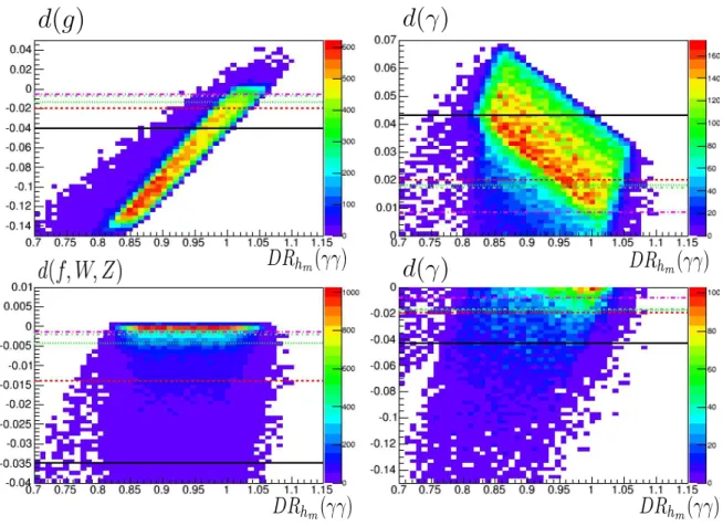
FIG. 1: (a) The distribution of the model points in d(γ) vs mr plane and (b) d(γ) vs ξ plane at Λφ=10 TeV.
The quantity we measure directly at the LHC is the detection ratio. The deviations of the detection ratios of the fermions, W boson and Z boson from the SM predictions are common as the d(A) case and depend on the Higgs-radion mixing and FqKK. We call it as DRhm(f f, W W, ZZ). The measurement of DRhm(γγ) gives independent information because it also depends on loop effects of the KK modes of fermions and gauge bosons. Currently, there is relatively large positive deviation from the SM prediction in the γγ detection ratio in the ATLAS, while that in the CMS is smaller than the SM prediction.
(a) (b)
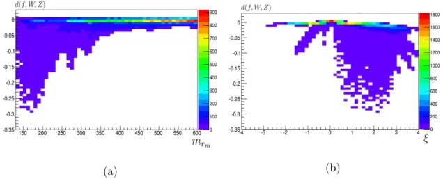
FIG. 2: (a) The distribution of the model points in d(f, W, Z) vs mr plane and (b) d(f, W, Z) vs ξ plane at Λφ=10 TeV.
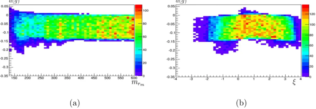
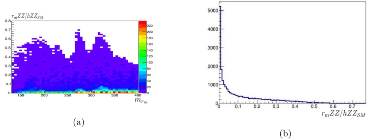
From now on, we show results of a parameter scan in the RS model. We generate model points which have uniform distribution between 130 GeV< mrm < 600 GeV, ξmin < ξ < ξmax,
0 < FtKK < 0.09, and 0 < FlKK < 0.083. Here, ξmaxand ξminare theoretical lower and upper bounds. We also fix Λφ=10 TeV and DRhm(γγ) > 0.7. Fig. 1, 2 and 3 show distribution of model points d(γ), d(f, W, Z) and d(g) vs (a) mass of radion-like state mrm and (b) the mixing parameter ξ respectively. In each figure, the color code represents the number of model points in the same bin. At the LHC, no other scalar boson for the 125 GeV Higgs boson has been discovered. Therefore, if the detection ratio of the mixed radion rm exceeds the 95% CL upper limit of the ATLAS and CMS Higgs searches [75, 76], we exclude those points from the figures. The discovery potential of rm at ILC will be discussed later.
The maximal value of d(γ) is about 0.06 in Fig. 1 and it is achieved for the small Higgs- radion mixing region (ξ ∼ 0). Most of the model points have |d(γ)| > 0.01, and the deviation may be detected if the ultimate sensitivity of δd(γ) = 0.83 % in Table II is achieved. The Higgs-radion mixing suppresses the coupling of hm to the SM particles. This can be seen in the d(f, W, Z) distribution in Fig. 2 where model points with large negative deviation are found for |ξ| * 0 and mrm < 250 GeV. In Fig. 1, 2, and 3 the lower limits of d(γ), d(f, W, Z), and d(g) are constrained by the condition that rm is not discovered by the current Higgs boson searches. In Fig. 3, we see that the KK quark contribution to d(g) is negative except at some exceptional points where mrm is close to mhm. Enhancement of d(g) for small mrm
is due to the trace anomaly contribution of g(rgg) through the Higgs-radion mixing. Indeed, the enhancement does not occur at ξ = 0, where the mixing is zero, and for very large |ξ| where the mixing reduces the Yukawa couplings significantly. For most of the parameter space, the deviation of the couplings is larger than the ultimate coupling sensitivity listed in Table. II.
d(g)
(a)
d(g)
(b)
FIG. 3: (a) The distribution of model points in d(g) vs mrplane, and (b) d(g) vs ξ plane at Λφ=10
TeV.