Vol. 5, 2011-20 | December 7, 2011 | http://dx.doi.org/10.5018/economics-ejournal.ja.2011-20
A New Method for Measuring Tail Exponents
of Firm Size Distributions
Shouji Fujimoto
Kanazawa Gakuin University
Atushi Ishikawa
Kanazawa GakuinUniversity
Takayuki Mizuno
University of Tsukuba
Tsutomu Watanabe
University of Tokyo
Abstract The authors propose a new method for estimating the power-law exponents of firm size variables. Their focus is on how to empirically identify a range in which a firm size variable follows a power-law distribution. On the one hand, as is well known a firm size variable follows a power-law distribution only beyond some threshold. On the other hand, in almost all empirical exercises, the right end part of a distribution deviates from a power-law due to finite size effects. The authors modify the method proposed by Malevergne et al. (2011). In this way they can identify both the lower and the upper thresholds and then estimate the power-law exponent using observations only in the range defined by the two thresholds. They apply this new method to various firm size variables, including annual sales, the number of workers, and tangible fixed assets for firms in more than thirty countries.
Special Issue
New Approaches in Quantitative Modeling of Financial Markets
JEL C16, C18, D20, E23
Keywords Econophysics; power-law distributions; power-law exponents; firm size variables; finite size effect
Correspondence Shouji Fujimoto, Kanazawa Gakuin University, The Department of Informatics and Business, 10 Sue-machi Kanazawa, Ishikawa, Japan;
e-mail: [email protected]; [email protected]
Citation Shouji Fujimoto, Atushi Ishikawa, Takayuki Mizuno, Tsutomu Watanabe (2011). A New Method for Measuring Tail Eponents of Firm Size Distributions. Economics: The Open-Access, Open-Assessment E-Journal, Vol. 5, 2011-20. http://dx.doi.org/10.5018/economics-ejournal.ja.2011-20
© Author(s) 2011. Licensed under a Creative Commons License - Attribution-NonCommercial 2.0 Germany
Introduction
Power-law distributions are frequently observed in social phenomena (e.g., Pareto (1897); Newman (2005); Clauset et al. (2009)). One of the most famous examples in Economics is the fact that personal income follows a power-law, which was first found by Pareto (1897) about a century ago, and thus referred to as Pareto distribution. Specifically, the probability that personal income x is above x0 is given by
P>(x)∝x−µ for x> x0 (1)
whereµ is referred to as a Pareto exponent or a power-law exponent.
As for the variables related to firm behavior, it is well known that there are several variables that follow a power-law, including firm sales for a particular period (e.g., annual sales), the number of workers employed by a firm, and the amount of fixed assets, like machinery equipments, held by a firm. The fact that the firm size variables mentioned above follow power-law distributions implies that the behavior of these variables at the aggregate level is dominantly affected by a very small number of firms that are extremely large in their size.
The purpose of this paper is to propose a new method for estimating the power- law exponent of a distribution. Our special focus is on how to empirically deter- mine a range in which a variable follows a power-law distribution. On the one hand, as shown in equation (1), a variable follows a power-law distribution only when it exceeds some threshold, for example x0in (1); the variable deviates from a power-law below that threshold. Thus we need to empirically specify where such a threshold exists. On the other hand, in almost all empirical exercises, the right end part of a distribution deviates from a power-law due to the limited number of observations. It is often the case that the right end part of a distribution exhibits a much quicker decay than implied by a power-law due to such a finite size effect. We need to eliminate that part of a distribution before estimating a power-law ex- ponent. Our strategy is to empirically specify the range of a variable, which is defined by a lower threshold x0 and an upper threshold x1, and then estimate a power-law exponent using only observations only in that range.
Our method is based on the one proposed by Malevergne et al. (2011).1 They propose to test the null hypothesis that, beyond some threshold, the upper tail of a distribution is characterized by a power law distribution against the alternative that the upper tail follows a lognormal beyond the same threshold.2It is important to note that their intention was to detect a lower threshold x0by conducting this test, and that they did not pay any particular attention to the presence of an upper threshold x1. However, as we will show later, in applying this method to firm size variables, one often encounters a situation that the threshold detected by this method is not x0but x1. Needless to say, this failure leads to an imprecise estimate of a power-law exponent.
In our method, we first apply the test by Malevergne et al. (2011) to detect a upper threshold, x1. We then repeat the test, but we “thin out” observations before conducting the second round test. Specifically, we discard observations above x1, which is detected by the first round test, and similarly we thin out observations below x1. Then we apply the test to the thinned out set of observations to detect x0.
The rest of this paper is organized as follows. In Section 1, we will provide detailed explanation on our new method. In Section 2, we will apply the new method to firm size variables, including annual sales, the number of workers, and tangible fixed assets for firms in more than thirty countries. Section 3 concludes the paper.
1 Methodology
Let us start by showing the empirical distributions for tangible fixed assets, which is denoted by K, the number of workers, L, and annual sales, Y . The cumulative distributions for these three variables for Japanese firms are shown in Figure 1 with horizontal and vertical axes being in logarithm. We see that dots are on a straight line in each of the three figures, indicating that each of the distributions is a power-law. However, dots deviate from a straight line when the firm size
1 See, for example, Hisano and Mizuno (2011) for an application of their method.
2 An alternative method to detect departures in the tails from the hypothesized probability distribu- tion is to use Anderson-Darling statistic (Coronel-Brizio and Hernandez-Montoya (2005, 2010)).
variables take very small or very large values. In other words, K, L, and Y follow power-law distributions only within some range. That is,
P>(K)∝K−µK for K0< K < K1, (2) P>(L)∝L−µL for L0< L < L1, (3) P>(Y )∝Y−µY for Y0< Y < Y1. (4) The main issue of this paper is how to estimate the range in which dots are on a straight line; namely,[K0, K1], [L0, L1], and [Y0,Y1].
10−6 10−4 10−2 100
100 102 104 106 108
P>(K)
P/AK(inthousandUSdollars )
2004 2005 20062007 20082009
(a) CDFs of tangible fixed as- sets in 2004–2009
10−6 10−4 10−2 100
100 102 104 106
P>(L)
TheNumberofEmployeeL 2000
20012002 20032004 2005 20062007 20082009
(b) CDFs of the number of workers in 2000–2009
10−6 10−4 10−2 100
100 102 104 106 108 P>(Y)
SalesY(inthousandUSdollars ) 2000
20012002 20032004 2005 20062007 20082009
(c) CDFs of annual sales in 2000–2009
Figure 1: Cumulative Distribution Functions of Firm Size Variables for Japanese Firms.
Our method is based on Malevergne et al. (2011), which propose a method to identify the boundary between a power-law and a lognormal. Consider a case described by equation (1). For each value of x, they test the null hypothesis that x follows a power-law distribution beyond that value against the alternative that x follows a lognormal distribution beyond the same value. They start this test for the maximum value of x, and repeat the test for the second largest, the third largest values, and so on, until the null is finally rejected.
Note that their test is equivalent to testing the null that the upper tail of the log of x follows an exponential distribution against the alternative that the log of x follows a truncated normal distribution. For this transformed test, del Castillo and Puig (1999) have shown that the clipped empirical coefficient of variation provides the uniformly most powerful unbiased test.
Specifically, let us consider a random variable z which follows a truncated normal distribution with truncation occurring at z= A. The probability density function P(z) is given by
P(z;α,β) = exp[−α(z − A) −β(z − A)2]/NC(α,β) (5) where NC(α,β) represents a scaling value, and it is defined by
NC(α,β) =
√π β exp
(α2 4β
)[ 1−Φ
( α
√2β )]
(6) whereΦ(·) is the CDF of a standard normal distribution. Note that it can be shown by using asymptotic expansion that P(z;α,β) →αexp[−α(z − A)] as (α,β) → (α, 0).
Suppose there are n observations for z (namely, z1, z2, ···, zn). The log likeli- hood is given by
l(θ) = l(α,β) = −α
∑
n i=1(zi− A) −β
∑
n i=1(zi− A)2− nlogNC(α,β) (7) and the maximum likelihood estimate forθ= (α,β) is characterized by
−γh(γ) +γ2+ 1/2
(h(γ) −γ)2 − 1 = c
2 (8)
whereγ and h(γ) are defined by
γ≡α/2√β; h(γ) ≡ exp(−γ2)
2√π(1 −Φ(√2γ)) (9)
and c2is the square of the coefficient of variation for(xi− A), which is defined by c2=⟨(x − A)
2⟩ − ⟨x − A⟩2
⟨x − A⟩2 =
⟨(x − A)2⟩
⟨x − A⟩2 − 1 (10)
where ⟨·⟩ represents the sample mean. For a give value of A, one can calculate c2 from the data, and then obtain a maximum likelihood estimate of γ from (8), which is denoted by ˆγ. Note that the expression on the left hand side of (8) is
monotonically increasing with respect toγ, so that one can obtain a solution just by applying a simple method like the Newton-Raphson method.
If z follows an exponential distribution rather than a truncated normal distribu- tion,β in equation (5) is equal to zero, and the log likelihood is given by
l(θ) = l(α, 0) = −α
∑
n i=1(xi− A) − nlog(α) (11)
The maximum likelihood estimate forθ is given by ˜θ= ( ˜α, 0) = (1/ ⟨x − A⟩, 0). Then the null hypothesis that z is exponentially distributed can be tested against the alternative that z follows a truncated normal distribution by conducting a like- lihood ratio test, in which the likelihood ratio is given by
W= 2(l( ˆθ) − l( ˜θ)) (12)
The random variable z is more likely to follow a truncated normal distribution if the value of W is above zero, and it is more likely to be exponentially distributed if W is below zero. Specifically, it is known that the asymptotic distribution of W around W = 0 is a 50-50 mixture of aχ2distribution with a degree of freedom of one, and a constant zero (see Self and Liang (1987) and Geyer (1994)). Therefore, the asymptotic distribution of W is given by W( ˆγ) = 0 if c is greater than unity, and
W( ˆγ) = n[2 log{2h( ˆγ)(h( ˆγ) − ˆγ)} + 2 ˆγ2− 2 ˆγh( ˆγ) + 1] (13) if c is less than unity. del Castillo and Puig (1999) adopts a more precise approxi- mation to W by using
W∗= W ( ˆγ) + 2L( ˆγ) + L2( ˆγ)/W ( ˆγ) (14) where L(·) is defined by
L( ˆγ) = 1 2log
[ 2 ˆγ3h( ˆγ) − 4 ˆγ2h( ˆγ)2+ ˆγh( ˆγ)(2h( ˆγ)2+ 3) − 3h( ˆγ)2+ 1 4(h( ˆγ) − ˆγ)2(W ( ˆγ)/n)
] (15) In sum, the procedure proposed by del Castillo and Puig (1999) and Malevergne et al. (2011) is as follows.
1. Pick up the largest n observations and take log. Set the threshold A equal to the log of the value for the largest observation.
2. Compute ˆγby solving (8).
3. Compute W∗and p-value associated with it by inserting the value of ˆγ into (14).
4. Repeat this procedure for n= 1, 2, 3, . . . until the p-value associated with W∗is sufficiently large to reject the null hypothesis.
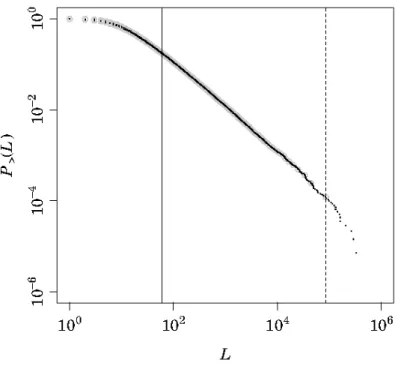
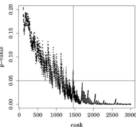
Let us show how the method proposed by Malevergne et al. (2011) works by applying it to the distribution for the number of workers employed by Japanese firms in 2004. The black dots in Figure 2 represent empirical CDF produced using actual observations. There are two vertical lines in the figure, but the dashed line represents the threshold identified by the procedure proposed by Malevergne et al. (2011), which corresponds to the 17th largest observation with the value (i.e., the number of workers) of 84,899. Figure 3a shows the p-value for each rank in this test. If their method works well, this result indicates that the number of workers follows a power-law beyond this threshold, but a lognormal below it. However, as one can clearly see from the figure, the black dots are on a straight line even below this threshold, implying that their method fails to detect a correct threshold. This failure happens because the right end part of the distribution decays quicker than the other part of the distribution due to the limited number of observations. The possibility of such a finite size effect is not seriously considered in Malevergne et al. (2011). It is important to note that this particular case is not an exception, but in fact we encounter similar failures quite often in estimating the power-law exponents of firm size distributions.
To cope with this problem, we propose to modify their procedure in the follow- ing way. Basically what we will do is to “thin out” observations so as to minimize the extent to which one suffers from the finite size effect. Specifically, after detect- ing the 17th largest observation as a (wrong) threshold, we discard 16 observations above it. We also discard the 18th, 19th, 20th,. . ., and 33rd largest observations, the 35th, 36th, 37th,. . ., and 50th largest observations, and so on. By repeating this procedure, we end up with a thinned out set of observations which consist of
Figure 2: Cumulative Distribution Function for the Number of Workers Employed by Japanese Firms in 2004. Black dots represent the original set of observations, while grey dots represent the thinned-out set of observations. The two vertical lines indicate the upper and lower thresholds, which are estimated using the method described in the text. The power-law exponent is estimated using only observations within the range defined by these two thresholds.
the 17th largest observation, the 34th largest observation, the 51st largest observa- tion, and so on. These thinned out observations are indicated by grey circles in Figure 2. Then we apply again the method by Malevergne et al. (2011), but this time not to the original set of observations but to the thinned out set of observa- tions. This second round test identifies a new threshold, which is represented by
(a) The p-value for each rank obtained from the first round test. The vertical line repre- sents the rank whose p-value falls below 5% threshold for the first time. The vertical line corresponds to the 17th largest observation.
(b) The p-value for each rank obtained from the second round test. The vertical line repre- sents the rank whose p-value is below the 5% threshold but the p-values associated with the ranks lower than that are all above the 5% threshold. The vertical line corresponds to the 1453rd largest observation.
Figure 3: The p-values obtained from the first and second round tests. The horizontal lines repre- sent the 5% threshold.
the vertical solid line in Figure 2. This corresponds to the 24701st largest among the original set of observations and the 1453rd largest among the thinned out set of observations. Figure 3b shows the p-value for each rank in this second round test. The number of workers corresponding to this second threshold is 60, which is substantially lower than the number corresponding to the first threshold. We see from the figure that dots, both black and grey, are on a straight line in the range indicated by the two vertical lines.
To see how our method works, consider a size-rank equation of the form
ln r= const −µln s (16)
where s represents a firm size, r is the rank associated with it, andµ is a power-law exponent. We assume that this size-rank equation holds for r∈ [r0, r1]. We know the value of r0 from the first round test (r0 is 17th in the above example). Let s0 represents the size associated with the rank r0. The constant term in equation (16) is equal to ln r0+µln s0. Therefore, equation (16) implies that
ln( r r0
)
= −µln( ss
0
)
(17) holds for r = r0, 2r0, 3r0, 4r0, . . . as far as r is smaller than r1. Thus we can estimate a power-law exponent µ using a thinned out set of observations {r0, 2r0, 3r0, 4r0, . . .}. Note that discarding only observations with higher ranks than r0 does not work, because, in this case, the rank in the new set of observa- tions is r− r0, rather than r/r0 in equation (17), and the log of r− r0 does not depend linearly on the log of s.
The procedure we propose is summarized as follows.
1. Apply the method proposed by Malevergne et al. (2011) to the original ob- servations to detect an observation (we refer to this as k-th largest observa- tion), above which the CDF is steeper than the other part due to finite size effect.
2. Create a new (thinned out) set of observations, consisting of the k-th largest observation, the 2k-th largest observation, the 3k-th largest observations, and so on.
3. Apply the method proposed by Malevergne et al. (2011) to the thinned out set of observations to detect a new threshold (we refer to this as K-th largest observations).
4. Estimate the slope of a straight line within the range defined by the value associated with the k-th largest observation and the value associated with the K-th largest observation.
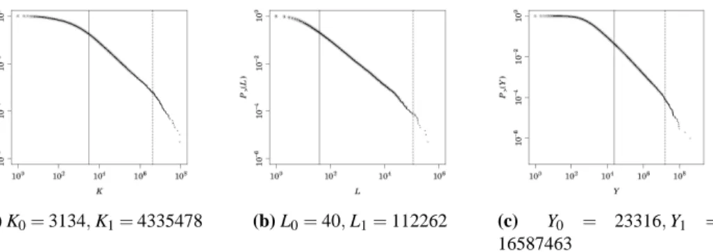
(a) K0= 3134, K1= 4335478 (b) L0= 40, L1= 112262 (c) Y0 = 23316, Y1 = 16587463
Figure 4: CDFs of K, L, and Y for Japanese Firms in 2007
(a) K0= 180, K1= 6167360 (b) L0= 4, L1= 119340 (c) Y0 = 12196, Y1 = 21357217
Figure 5: CDFs of K, L, and Y for French Firms in 2007
2 Empirical Results
In this section we apply the new method to firm size variables, including annual sales, the number of workers, and tangible fixed assets for firms in more than
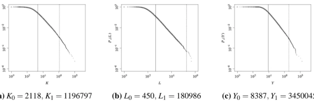
(a) K0= 2118, K1= 1196797 (b) L0= 450, L1= 180986 (c) Y0= 8387, Y1= 3450045 Figure 6: CDFs of K, L, and Y for Chinese Firms in 2007
thirty countries.3 The data comes from ORBIS provided by Bureau van Dijk, which contains B/S and P/L information for more than 60 million firms all over the world. The sample includes the period from 1999 until 2009.4
Figure 4 shows the CDFs for tangible fixed assets, the number of workers, and annual sales for Japanese firms in 2007. As emphasized in the previous sections, dots are not always on a straight line; namely, there is a range in which dots are on a straight line, but dots deviate from the straight line below the lower bound of the range, and they also deviate from the straight line beyond the upper bound of the range. Our estimation result indicates that, for tangible fixed assets, the lower bound of the range, K0, is 3,134 thousand USD, and the upper bound of the range, K1, is 4,335,478 thousand USD. The range is shown by two vertical lines, and we see that dots are on a straight line inside the range, but dots deviate from it outside the range, indicating that our estimation procedure works well in identifying upper and lower bounds. We confirm the same results for the number of workers as well as for annual sales. Figure 5 and Figure 6 show the results for French firms and
3 There is a long list of papers that investigate various aspects of firm size distributions, includ- ing Stanley et al. (1995), Okuyama et al. (1999), Ramsden and Kiss-Haypál (2000), Mizuno et al. (2006), Axtell (2001), Gaffeo et al. (2003), Fujiwara et al. (2004), and Zhang et al. (2009).
4 More detailed information on the dataset employed in this paper is available at http://www.bvdinfo.com/Home.aspx.
year µK µL µY
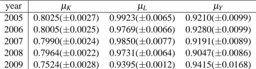
2005 0.8025(±0.0027) 0.9923(±0.0065) 0.9210(±0.0099) 2006 0.8005(±0.0025) 0.9769(±0.0066) 0.9280(±0.0099) 2007 0.7990(±0.0024) 0.9850(±0.0077) 0.9191(±0.0089) 2008 0.7964(±0.0022) 0.9731(±0.0064) 0.9047(±0.0086) 2009 0.7524(±0.0028) 0.9395(±0.0012) 0.9415(±0.0168)
Table 1: The estimates of power-law exponents for tangible fixed assets (µK), the number of work- ers (µL), and annual sales (µY) for Japanese firms
those for Chinese firms, indicating again that our estimation procedure works well in identifying upper and lower bounds of a range.
After identifying upper and lower bounds of a range, we estimate the slope of CDF by applying an OLS regression. The results for Japan is presented in Table 1. The table shows the power-law exponents for tangible fixed assets, the number of workers, and annual sales, each of which is denoted by µK, µL, and µY. For example, the power-law exponent for tangible fixed assets in 2005 is 0.8025 and its standard error is 0.0027, suggesting a high precision of the estimate. We also see that each of the three exponents is fairly stable over time.
One of the interesting findings we learn from the table is thatµK tends to be the smallest among the three, andµLtends to be the largest among the three. Put differently, there exists a relationship betweenµK,µL, andµY such that
µK<µY <µL (18)
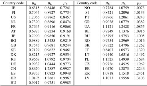
We conduct the same exercise for other countries, and the result is reported in Table 2. It shows that the estimates of power-law exponents differ across countries, but there still exist some tendency thatµK<µY<µLfor each country.
Why does equation (18) hold? One way to address this question is to start from a Cobb-Douglas production function, which is of the form
Y = AKαLβ (19)
Country code µK µL µY Country code µK µL µY
IE 0.6315 0.8446 0.7241 NO 0.7784 1.0759 1.0073
FI 0.7044 0.8927 0.7734 SI 0.8421 1.2096 1.0133
US 1.2056 0.8862 0.8457 PT 0.8966 1.2061 1.0243
NL 0.7390 0.8896 0.8474 GR 0.9028 1.0779 1.0382
FR 0.7645 0.9116 0.9068 UA 1.1121 1.2428 1.0855
AT 0.6925 0.8234 0.9168 BE 0.8249 1.1376 1.0916
JP 0.7990 0.9850 0.9191 RU 0.8795 1.5753 1.1005
BG 0.9889 1.5435 0.9219 RO 0.9754 1.2969 1.1016
GB 0.7545 0.9681 0.9244 SK 0.9322 1.4796 1.1262
SE 0.7129 0.9622 0.9461 IT 0.8403 1.0573 1.1320
DK 0.8215 0.9927 0.9554 LT 0.9440 1.6516 1.1492
RS 0.9668 1.0792 0.9704 PL 1.1525 1.4939 1.1684
DE 0.9932 1.0444 0.9773 CZ 0.9726 1.4525 1.1962
CN 0.8670 1.2887 0.9927 EE 1.0470 1.2875 1.2246
ES 0.9355 1.0823 0.9948 KR 1.0718 1.1518 1.2451
HR 1.0195 1.2881 0.9967 LV 1.1073 1.5558 1.3103
HU 0.9917 0.9751 0.9985
Table 2: The estimates of power-law exponents for tangible fixed assets (µK), the number of work- ers (µL), and annual sales (µY) for firms in 33 countries in 2007. Country Code: IE IRELAND, FI FINLAND, US UNITED STATES, NL NETHERLANDS, FR FRANCE, AT AUSTRIA, JP JAPAN, BG BULGARIA, GB UNITED KINGDOM, SE SWEDEN, DK DENMARK, RS SER- BIA, DE GERMANY, CN CHINA, ES SPAIN, HR CROATIA, HU HUNGARY, NO NORWAY, SI SLOVENIA, PT PORTUGAL, GR GREECE, UA UKRAINE, BE BELGIUM, RU RUSSIAN FEDERATION, RO ROMANIA, SK SLOVAKIA, IT ITALY, LT LITHUANIA, PL POLAND, CZ CZECH REPUBLIC, EE ESTONIA, KR KOREA, REPUBLIC OF and LV LATVIA.
whereαandβare positive (but less than unity) parameters.5 This equation simply says that the amount of output produced by a firm is determined by the amount of inputs, i.e., labor and capital inputs, employed by the firm, as well as the level of productivity of the firm, which is denoted by A in equation (19). Given that Y , K, and L all follow power-law distributions, equation (19) implies
µY = min
{µ
K
α ,µβL }
(20)
5 See Cobb and Douglas (1928) for more on the Cobb-Douglas production function.
if K and L are independent.6 A simple comparison of (20) and (18) suggests a way to know where (18) comes from. Suppose that the sum ofαandβ equals to unity as is often assumed in the literature in Economics. The value ofµK,µL, andµYfor
2005 in Japan is 0.8025, 0.9923, 0.9210, respectively. These empirical estimates of power-law exponent are consistent with (20) ifα = 0.87 andβ = 0.13.7 Note that this calculation is nothing more than an illustration since the assumptions adopted above may not necessary be satisfied in the actual data; namely, K and L may not necessarily be independent, and the sum ofαandβ may not necessarily be equal to unity. However, this calculation still suggests a way to reconcile the different empirical estimates of power-law exponents for tangible fixed assets, the number of workers, and annual sales. See Mizuno et al. (2011) for more empirical results and discussion along this line of research.
3 Conclusion
We have proposed a new method for estimating the power-law exponent of a firm size variable, such as annual sales. Our focus is on how to empirically identify a range in which a firm size variable follows a power-law distribution. It is well known that a firm size variable follows a power-law distribution only beyond some threshold. On the other hand, in almost all empirical exercises, the right end part of a distribution deviates from a power-law due to finite size effect. We modify the method proposed by Malevergne et al. (2011) so that we can identify both of the
6 Jessen and Mikosch (2006) provide a compact summary of various properties of power law distri- butions. One of them indicates that K/αfollows a power-law and its exponent isµK/α. Similarly, the power-law exponent for L/β isµL/β. Also we know from Jessen and Mikosch (2006) that the product of two power-law variables is again a power-law and its exponent is equal to the smaller one of the two exponents associated with the two variables. We obtain equation (20) by combining these properties. See Mizuno et al. (2011) for further discussions and empirical evidence on this property.
7 Given these parameter values, µαK= 0.921 andµβL = 7.633, so that min{µαK,µβL}= 0.921, which is identical to the empirical value ofµY.
lower and the upper thresholds and then estimate the power-law exponent using observations only in the range defined by the two thresholds.8
Malevergne et al. (2011) propose to test the null hypothesis that, beyond some threshold, the upper tail of a distribution is characterized by a power law distri- bution against the alternative that the upper tail follows a lognormal beyond the same threshold. It is important to note that their intention was to detect a lower threshold by conducting this test, and that no attention was paid to the presence of an upper threshold. In our method, we first apply the test by Malevergne et al. (2011) to detect a upper threshold. We then repeat the test, but we “thin out” observations before conducting the second round test. Specifically, we discard observations above the upper threshold, which is detected by the first round test, and similarly we thin out observations below the upper threshold. Then we apply the test to the thinned out set of observations to detect a lower threshold.
We have applied this new method to various firm size variables, including annual sales, the number of workers, and tangible fixed assets for firms in more than thirty countries. First, we find that our new method works well in identifying upper and lower thresholds. Second, we find that there exits robust tendency in each country that the exponent for tangible fixed capital is the lowest, the exponent of annual sales is the second lowest, and the exponent of the number of workers is the largest. We provide a tentative argument based on a Cobb-Douglas production function to explain the observed difference in the three power-exponents.
Details on Numerical Calculation
In this appendix we will provide more details about how to numerically solve equation (9) and the other related equations. Error functions built in programming languages sometimes fail to solve these equations due to underflow. To illustrate
8 In this paper, we identify upper and lower thresholds, and discard observations above and below the thresholds. However, the observations exceeding the upper threshold, i.e. the most extreme observations, may contain some useful information on firm size distributions, or more generally on firm dynamics. It is our future task to carefully examine the properties of these most extreme observations.
this, consider a function of the form f(x) = exp(x2){1−Φ(√2x
)}
∼ 1
2√π
∑
∞ k=0(−1)k(2k − 1)!!2k x2k+11
Note that the function f(·) is basically the same function as h(·) in (9). The second row of this equation is obtained by asymptotic expansion. Figure 7a compares the result obtained from a built-in error function and the result obtained using the equation resulting from asymptotic expansion (up to x to the 25th power). We see that the built-in error function is able to return a precise outcome up to x= 6, but unable to do so for the values greater than that due to underflow. To fix this problem, we use a built-in error function for up to x= 4, but use an equation obtained from asymptotic expansion for x> 4.
Turning to a function L(·) in equation (15), we compare in Figure 7b the result obtained from a built-in error function and the result obtained using asymptotic expansion up to x to the 25th power. Again we see that the built-in error function fails to return a precise outcome for x greater than 4. More importantly, there is a discontinuous jump around at x= 4, which cannot be completely eliminated even if we increase the order of expansion. To fix this, we use the built-in function for x< 4 and use an equation obtained from asymptotic expansion for x > 5, and adopt a linear extrapolation between the two. Also we set an approximate value of L(x) for x > 15 at zero since it can be shown analytically that L(x) → −0 as x→∞.
Finally, a similar problem occurs for L(x)2/W (x) in equation (14). We use the built-in function for x< 4 and use an equation obtained from asymptotic ex- pansion for x> 6, and adopt a linear extrapolation between the two. We also set an approximate value of L(x)2/W (x) at 64/9 for x > 10 since it can be shown analytically that L(x)2/W (x) → 64/9 as x →∞.
(a) Black line represents f(x) in (21) com- puted using a built-in error function; Gray line represents the same function f(x), but it is computed using an equation obtained from asymptotic expansion equation (up to x to the 25th power).
(b) Black line represents L(x) in (15) com- puted using a built-in error function; Gray line represents the same function L(x), but it is computed using an equation obtained from asymptotic expansion equation (up to x to the 25th power).
Figure 7: Comparison between the result from built-in error function and the result from asymp- totic expansion
References
Axtell, R. (2001). Zipf Distribution of U.S. Firm Sizes. Science, 293: 1818–1820.
URLhttp://linkage.rockefeller.edu/wli/zipf/axtell01.pdf.
Clauset, A., Shalizi, C., and Newman, M. (2009). Power-Law Distributions in Empirical Data. SIAM Review, 51: 661–703. URL http://arxiv.org/abs/arxiv: 0706.1062.
Cobb, C., and Douglas, P. (1928). A Theory of Production. American Eco- nomics Review, 18: 139–165. URLhttp://www.aeaweb.org/aer/top20/18.1.139- 165.pdf.
Coronel-Brizio, H., and Hernandez-Montoya, A. (2005). On Fitting the Pareto– Levy Distribution to Stock Market Index Data: Selecting a Suitable Cutoff Value. Physica A, 354: 437–449. URLhttp://arxiv.org/abs/cond-mat/0411161. Coronel-Brizio, H., and Hernandez-Montoya, A. (2010). The Anderson-Darling
Test of Fit for the Power Law Distribution from Left Censored Samples. Phys- ica A: Statistical Mechanics and its Applications, 389(3): 3508–3515. URL
http://arxiv.org/abs/1004.0417.
del Castillo, J., and Puig, P. (1999). The Best Test of Exponentiality against Singly Truncated Normal Alternatives. Journal of the American Statistical Association, 94(446): 529–532.
Fujiwara, Y., Guilmi, C. D., Aoyama, H., Gallegati, M., and Souma, W. (2004). Do Pareto–Zipf and Gibrat Laws Hold True? An Analysis with European Firms. Physica A, 335: 197–216. URLhttp://chemlabs.nju.edu.cn/Literature/ Zipf/Do%20Pareto-Zipf%20and%20Gibrat%20laws%20hold%20true-An% 20analysis%20with%20European%20firms%20.pdf.
Gaffeo, E., Gallegati, M., and Palestrinib, A. (2003). On the Size Distribu- tion of Firms: Additional Evidence from the G7 Countries. Physica A, 324: 117–123. URLhttp://www.mendeley.com/research/on-the-size-distribution-of- firms-additional-evidence-from-the-g7-countries/.
Geyer, C. (1994). On the Asymptotics of Constrained M-Estimation. The Annals of Statistics, 22: 1993–2010. URLhttp://www.jstor.org/stable/2242495.
Hisano, R., and Mizuno, T. (2011). Sales Distribution of Consumer Electronics. Physica A, 390: 309–318. URLhttp://arxiv.org/abs/1004.0637.
Jessen, A. H., and Mikosch, T. (2006). Regularly Varying Functions. Publications de l’Institut Mathematique, Nouvelle serie, 80(94): 171–192.
Malevergne, Y., Pisarenko, V., and Sornette, D. (2011). Testing the Pareto against the Lognormal Distributions with the Uniformly Most Powerful Unbiased Test Applied to the Distribution of Cities. Physical Review E, 83: 036111.URLhttp:
//www.mendeley.com/research/testing-pareto-against-lognormal-distributions- uniformly-most-powerful-unbiased-test-applied-distribution-cities/.
Mizuno, T., Katori, M., Takayasu, H., and Takayasu, M. (2006). Statistical and Stochastic Laws in the Income of Japanese Companies. In H. Takayasu (Ed.), Empirical Science of Financial Fluctuations: The Advent of Econophysics.URL
http://arxiv.org/ftp/cond-mat/papers/0308/0308365.pdf.
Newman, M. (2005). Power Laws, Pareto Distributions and Zipf’s law. Contempo- rary Physics, 46: 323–351. URLhttp://arxiv.org/PS_cache/cond-mat/pdf/0412/ 0412004v3.pdf.
Okuyama, K., Takayasu, M., and Takayasu, H. (1999). Zipf’s Law in Income Dis- tribution of Companies. Physica A, 269: 125–131. URLhttp://www.mendeley. com/research/zipfs-law-income-distribution-companies/.
Pareto, V. F. D. (1897). Cours d’Economique Politique. London: Macmillan. Ramsden, J., and Kiss-Haypál, G. (2000). Company Size Distribution in Different
Countries. Physica A, 277: 220–227.
Self, S., and Liang, K.-Y. (1987). Asymptotic Properties of Maximum Likelhood Estimatiors and Likelihood Ratio Test Under Nonstandard Conditions. Journal of the American Statistical Association, 82(398): 605–610. URLhttp://www. jstor.org/stable/2289471.
Stanley, M. H. R., Buldyrev, S. V., Havlin, S., Mantegna, R. N., Salinger, M. A., and Stanley, H. E. (1995). Zipf plots and the size distribution of firms. Economics Letters, 49: 453–457.URLhttp://ideas.repec.org/a/eee/ecolet/ v49y1995i4p453-457.html.
Zhang, J., Chen, Q., and Wang, Y. (2009). Zipf distribution in top Chinese Firms and an Economic Explanation. Physica A, 388: 2020–2024. URLhttp://www. sciencedirect.com/science/article/pii/S0378437109000806.
Please note:
You are most sincerely encouraged to participate in the open assessment of this article. You can do so by either recommending the article or by posting your comments.
Please go to:
http://dx.doi.org/10.5018/economics-ejournal.ja.2011-20
The Editor
© Author(s) 2011. Licensed under a Creative Commons License - Attribution-NonCommercial 2.0 Germany