he Importance of Understanding Bidirectional Relationships
to Uncover the Role of the Sex Gap in Life Expectancy in
National Happiness Indicators
Junji Kageyama
Acknowledgement
I wish to thank participants in both the Meikai Economic Workshop and International Conference
“Determinants of Unusual and Differential Longevity” at Austrian Academy of Sciences. I also wish to thank the Miyata Research Fund of Meikai University for financial support. Any remaining errors are my own.
Abstract
The relationships between happiness indicators and the sex gap in life expectancy are bidirectional and complex, causing national average happiness to positively correlate to the happiness gap between women and men in European countries. This paper assesses the importance of recognizing the bidirectional relationships between these happiness indicators and the life expectancy gap, and, thus, of controlling for the simultaneous effects, to reveal the role that the life expectancy gap plays in this positive correlation. For this aim, this paper employs regression analysis and compares the results under IV and OLS estimation. The results show that, without fully understanding the bidirectional relationships, we are unable to detect expected relationships in two out of three regression models, failing to uncover the role of the life expectancy gap. These results point to the existence of mutual interdependence between demography and happiness studies.
Key words: life expectancy, sex difference, subjective well-being, happiness
1. Background
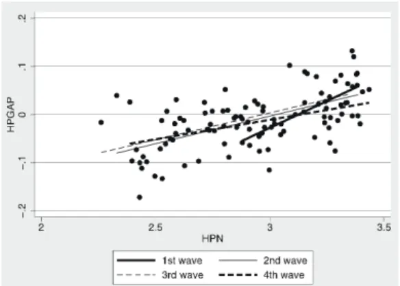
As presented in Figure 1, national average happiness (HPN) and the happiness gap between women and men (HPGAP) are positively correlated in European countries (European and World Values Surveys, Waves 1 to 4). In happier countries, women are, on average, particularly happier.
At the first glance, this correlation seems to be an issue relevant only in happiness studies. However, this is in fact a demographic issue since the intermediary connecting these two variables is the difference in life expectancy between women and men (LEGAP).
This is rooted in the findings in Kageyama
(2012), which empirically showed that the relationships between LEGAP and these happiness indicators are bidirectional. In one direction, LEGAP negatively affects both HPN and HPGAP. An increase in LEGAP raises women’s widowhood ratio, and, since widows are, on average, less happy, it lowers women’s average happiness, HPN, and HPGAP. We call this effect the “marital-status composition effect” as the marital-status composition plays a central role.
In the opposite direction, HPN and HPGAP individually affect LEGAP. HPN, on one hand, negatively influences LEGAP. Since men are more fragile in the sense that their mortality responds more elastically to stress than their female counterpart, a decline in HPN raises men’s mortality relative to women’s and widens LEGAP as long as the happiness data capture stress level.1 In this paper, we call this effect the “male-fragility effect”.
HPGAP, on the other hand, is expected to positively affect LEGAP. As previous studies have shown, happier individuals are healthier (see Pressman and Cohen 2005 and Veenhoven 2008 for reviews), and we can expect that the same relationship holds at the gender level. We call this effect the “happy- survival effect” in this paper. These three effects are summarized in the diagram in Figure 2.
By re-ordering these relationships, we can hypothesize that HPN and HPGAP are positively correlated. First, due to the male-fragility effect, a lower HPN leads to a greater LEGAP. Next, due to the marital-status composition effect, a greater LEGAP lowers HPGAP as well as HPN. By putting these effects together, we can expect that a lower HPN corresponds to a lower HPGAP, generating the positive correlation as demonstrated in Figure 1.
1 “Women get sick and men die (Nathanson 1977, p.14)” summarizes this effect. See also McKee and Shkolnikov 2001, Luy and Di Giulio 2006, and Phillips 2006 for how behavioral factors and lifestyle affect the sex difference in life expectancy.
Figure 1: The Relationship between HPN and HPGAP
Source: Kageyama(2013)
Figure 2: Causal Relationships
Kageyama (2013) tested this hypothesis. Employing regression analysis, it showed that, after accounting for repercussive effects, the hypothesis given above explains one-third of the correlation between HPN and HPGAP.
Kageyama (2013), however, did not assess the criticality of being aware of and, thus, of controlling for the simultaneous effects. To fill this gap, the present study tests the importance of understanding the bidirectional relationships. Specifically, it asks if we could detect the relationships among LEGAP, HPN, and HPGAP, and reveal the role of LEGAP in the correlation between HPN and HPGAP without controlling for the bidirectional relationships. By doing this, we can further assess the importance of demographic knowledge in happiness studies, and of the understanding of happiness in demography.
The results point to the importance of controlling for bidirectional relationships, without which, we are unable to find the expected relationships in two out of three regression models, resulting in the failure to uncover the role of LEGAP in the correlation between HPN and HPGAP. These results suggest that, to uncover the role of LEGAP, it is insufficient to know how LEGAP operates beneath HPN and HPGAP. We also need to understand how HPN and HPGAP affect LEGAP.
The remainder of the paper is organized as follows. The next section performs regression analysis. The information on the data, such as data sources and sample countries, are presented in the appendix. Section 3 concludes.
2. Regression analysis
2. 1. Data, variables, and strategies This study follows Kageyama (2013). The data set contains 82 country-periods (36 countries) across four periods, due to the limited availability
of happiness data. The number of countries in each period is, respectively, 7(Period 1), 26(Period 2), 20(Period 3), and 29(Period 4). As the data set is heavily unbalanced, we treat it as a pooled data set.2
The happiness data are taken from the European and World Values Surveys, Waves 1(1981-84), 2
(1989-93), 3(1994-99), and 4(1999-2004). Among others, one question asks, “Taking all things together, would you say you are: very happy (4), quite happy
(3), not very happy (2), or not at all happy (1)?” In this data set, the average number of respondents with personal data covering age, sex, and marital status that can be separated into the married, the separated or divorced, the widowed, and the never married, is 1,282(687 women and 595 men) per country-wave. The largest number is 4,072(2,180 women and 1,892 men) in Spain (Wave 2), and the least is 359(191 women and 168 men) in Malta (Wave 2).
This study treats the data as cardinal, following Ferrer-i-Carbonell and Frijters (2004). Their study showed that, whereas happiness data are, by nature, ordinal, assuming cardinality makes little difference to the results. This finding adds support for using the averages of respondents as national indicators of happiness.3 The cross-country averages of HPN and HPGAP are respectively 2.97 and -0.07.
As for LEGAP, we use the difference in life expectancy at birth between women and men. Although this is not a perfect measure to examine the relationship between longevity and happiness because life expectancy
2 The results obtained in the present study are consistent with previous studies, such as Pampel and Zimmer (1989) and Ram (1993), that employ panel data sets.
3 While the reliability of happiness data is still being de- bated, the accumulating evidence in happiness studies supports the use of these data for academic research. Hel- liwell (2007), for example, showed that there is a strong negative correlation between suicide rate and life satisfac- tion, indicating that life satisfaction correctly reflects the mental condition. See also Clark and Senik (2011) for a review.
at birth includes children while happiness data do not, the data on life expectancy of adult cohorts are limited to even fewer countries. Thus, we employ life expectancy at birth as its proxy.
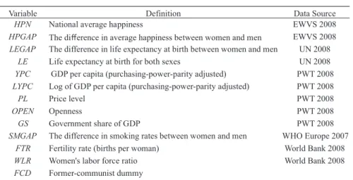
In addition, we need variables to control for cross-country differences in social and economic conditions. For this purpose, we incorporate the social and economic variables used in previous studies. These variables are presented in Table 1.
In terms of model specification, we employ three regression models. The first model aims to identify the marital-status composition effect and regresses HPGAP on HPN and LEGAP, controlling for social and economic variables. For the same purpose, the second model regresses HPN on HPGAP, LEGAP, and social and economic variables. Note that the second model does not intend to provide a thorough explanation for cross-country differences in HPN. The current data set is not suitable for this purpose as the sample size is too small. Finally, the third model aims to test the reverse effects of HPN and HPGAP on LEGAP to identify the male-fragility and happy-survival effects. Thus, it regresses LEGAP on HPN and HPGAP, controlling for social and economic variables.
For regressing these models, we depart from
Kageyama (2013) and use both the IV and OLS methods to evaluate the importance of controlling for the bidirectional relationships. The difference in results between these two methods shows the importance of such controls to find causal relationships.
With respect to instrumental variables, we use the sex difference in smoking rate (SMGAP) in the first two regression models to control for the reverse effects of HPN and HPGAP on LEGAP. While SMGAP is significantly correlated with LEGAP, it is not directly correlated with either HPGAP or HPN, making it a suitable instrument. Turning to the third regression model, we use happiness of the widowed and the happiness gap of the married for HPN and HPGAP. Controlling for marital status substantially reduces the marital-status composition effect running from LEGAP to HPN and HPGAP.4 In all regression models, the test scores for under- and weak- identification tests show no sign of
4 Among the four types of marital statuses, the ones for the widowed are the ideal instruments because the individuals in this category have already gone through the hardship of losing a spouse and LEGAP should not have any further impact on them. At the same time, however, the number of widows and widowers are very small in the survey. This makes the explanatory power of the happiness gap of the widowed weak in the first-stage regression, and, for this reason, we use the happiness gap of the married.
Variable Definition Data Source
HPN National average happiness EWVS 2008
HPGAP The difference in average happiness between women and men EWVS 2008 LEGAP The difference in life expectancy at birth between women and men UN 2008
LE Life expectancy at birth for both sexes UN 2008
YPC GDP per capita (purchasing-power-parity adjusted) PWT 2008 LYPC Log of GDP per capita (purchasing-power-parity adjusted) PWT 2008
PL Price level PWT 2008
OPEN Openness PWT 2008
GS Government share of GDP PWT 2008
SMGAP The difference in smoking rates between women and men WHO Europe 2007
FTR Fertility rate (births per woman) World Bank 2008
WLR Women's labor force ratio World Bank 2008
FCD Former-communist dummy
Table 1: Deinition of Variables
identification problems (Stock and Yogo 2005 and Kleibergen and Paap 2006), and support the validity of the instrumental variables.5
2. 2. Regression results
Table 2 presents the results for the HPGAP regression model. Whether or not control variables are included, LEGAP is significantly negative at least at the 10% level under IV estimation, supporting the existence of the marital-status composition effect.6 Under OLS estimation, however, LEGAP loses
5 The over-identification test (Hansen 1982) also supports the validity of the instruments. See Kageyama (2013) for details.
6 Period dummies are omitted in equations (1-3) because they are insignificant.
its explanatory power. Equation (1-1ols) shows that LEGAP is insignificant while HPN becomes significant. The same results hold in Equation (1- 2ols) in which the former-communist dummy
(FCD) and period dummies are included. Equation
(1-3ols) shows that, when social and economic variables are included, HPN loses its significance, but LEGAP remains insignificant. These results indicate that, without controlling for the happy- survival effect, i.e., the reverse effect of HPGAP on LEGAP, we are unable to detect the marital-status
(1-1) (1-2) (1-3)
IV OLS IV OLS IV OLS
HPN -0.006 0.088 0.053 0.124 0.005 0.039
-0.14 2.97 *** 1.13 3.19 *** 0.10 0.96
LEGAP -0.020 -0.005 -0.019 -0.006 -0.011 -0.005 -3.50 *** -1.30 -3.25 *** -1.48 -2.24 ** -1.51
YPC -0.0033 -0.0037
-2.66 *** -3.02 ***
PL 0.0016 0.0016
4.92 *** 5.02 ***
FTR 0.030 0.032
2.32 ** 2.36 **
OPEN 0.0002 0.0002
1.61 1.79 *
GS 0.0025 0.0019
2.66 *** 1.99 **
FCD 0.043 0.034 0.047 0.044
1.99 ** 1.84 * 2.36 ** 2.29 ** Period D excl. excl. incl. incl. excl. excl.
Under-ID 12.14 12.00 19.23
Test 0.00 0.00 0.00
Weak-ID 23.53 23.42 51.60
Test 16.38 16.38 16.38
R-sq 0.23 0.39 0.30 0.42 0.58 0.60
Note: The number of observation is 82. For the IV estimation, we use SMGAP as the instrument to contorl for the endogeneity related to LEGAP . The top figures are the estimated coefficients, and the bottom figures are heteroskedasticity-robust t-statistics. ***,
**, and * respectively indicate the significance level at p<0.01, p<0.05, and p<0.10. Under- ID test: Kleibergen-Paap rk LM statistic at the top, and the corresponding p-value at the bottom (Kleibergen & Paap, 2006). Weak-ID test: Kleibergen-Paap rk Wald F statistic at the top, the Stock-Yogo weak ID test critical value for the Cragg-Donald i.i.d. case for a 10% bias at the bottom (Kleibergen & Paap, 2006; Stock & Yogo, 2005). Eqs. (1-1iv) and (1-2iv) are from Kageyama (2013).
-3.50 ***
1.13
1.99 **
Table 2: Regression Results(Dependent Variable: HPGAP)
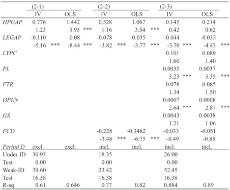
composition effect running from LEGAP to HPGAP. Table 3 presents the results for the HPN regression model. Under IV estimation, LEGAP is significantly negative at the 1% level in all equations, supporting the existence of the marital-status composition effect. Interestingly, the same is true under OLS estimation. These results suggest that the bias due to the endogeneity is not as obvious as the HPGAP regression model. Nevertheless, we are unable to draw any conclusions about the direction of the causality between HPN and LEGAP under OLS estimation as the expected effects are negative in both directions.
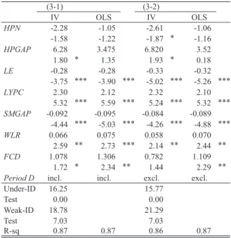
Finally, Table 4 presents the results for the LEGAP regression model. Equations (3-1) include period dummies, and equations (3-2) drop them as they are insignificant. In equation (3-2iv), both HPN and HPGAP are significant at the 10% level, supporting the existence of both the male-fragility and happy-survival effects and confirming the
existence of the reverse effects in the previous two regression models. Under OLS estimation, on the other hand, HPN and HPGAP become insignificant, and, instead, FCD increases its significance. These results indicate the importance of controlling for reverse causality. Without controlling for the marital- status composition effect, i.e., the reverse effects of LEGAP on HPN and HPGAP, we would conclude that the large life expectancy gaps in former- communist countries, at least partially, results from their unobservable social and political inheritance.
These results demonstrate that, without fully understanding the bidirectional relationships, we are unable to uncover the role that LEGAP plays in the correlation between HPN and HPGAP. Without controlling for the simultaneous effects, we cannot reject the null that LEGAP is neutral on HPGAP in the first regression model, or the nulls that HPN and HPGAP are neutral on LEGAP in the third regression model, resulting in the failure to connect
(2-1) (2-2) (2-3)
IV OLS IV OLS IV OLS
HPGAP 0.776 1.442 0.528 1.067 0.145 0.214
1.23 3.95 *** 1.16 3.54 *** 0.42 0.62
LEGAP -0.110 -0.08 -0.078 -0.035 -0.044 -0.035 -5.16 *** -8.44 *** -3.82 *** -3.77 *** -3.70 *** -4.43 ***
LYPC 0.101 0.089
1.60 1.40
PL 0.0035 0.0037
3.23 *** 3.35 ***
FTR 0.078 0.085
1.34 1.50
OPEN 0.0007 0.0008
2.64 *** 2.87 ***
GS 0.0043 0.0038
1.21 1.06
FCD -0.228 -0.3482 -0.033 -0.051
-3.48 *** -6.75 *** -0.49 -0.85 Period D excl. excl. incl. incl. incl. incl.
Under-ID 30.93 18.35 26.00
Test 0.00 0.00 0.00
Weak-ID 39.60 23.42 52.45
Test 16.38 16.38 16.38
R-sq 0.61 0.646 0.77 0.82 0.884 0.89
Note:Refer to Table 2. Eqs. (2-1iv) and (2-2iv) are from Kageyama (2013). Table 3: Regression Results (Dependent Variable: HPN)
LEGAP and HPGAP. In other words, to uncover the role of LEGAP, it is insufficient to know how LEGAP operates beneath HPN and HPGAP. We need to go step further and understand how HPN and HPGAP affect LEGAP.
3. Concluding remarks
This paper shows the importance of under- standing the bidirectional relationships between happiness and the sex difference in life expectancy to identify causal relationships running in between.
The results point to the existence of mutual interdependence between demography and happiness studies. Happiness indicators do not only depend on the sex gap in life expectancy, but also affect it. The same is true for the sex gap in life expectancy. This paper demonstrates that, to truly understand happiness, we need to study it in the context of demography, which,
in turn, requires an understanding of happiness. The importance of demography in happiness studies is particularly noteworthy. For one thing, demography addresses the relationships between demographic variables and happiness at the individual level. Examples of such studies include the relationship between health and happiness (e.g., Diener et al. 1999, Frey and Stutzer 2002, Helliwell 2003, Borooah 2006, Pressman and Cohen 2005, and Veenhoven 2008), and the relationship between happiness and fertility (e.g., Kohler et al. 2003, Clark et al. 2008, Parr 2010, Hansen 2012, and Myrskylä and Margolis 2012).
For another, demography plays a crucial role in understanding aggregate measures of happiness. As presented in this study, even to understand the relationship between national average happiness and its sex difference, we need demography. Demography operates beneath national indicators of happiness
(3-1) (3-2)
IV OLS IV OLS
HPN -2.28 -1.05 -2.61 -1.06
-1.58 -1.22 -1.87 * -1.16
HPGAP 6.28 3.475 6.820 3.52
1.80 * 1.35 1.93 * 0.18
LE -0.28 -0.28 -0.33 -0.32
-3.75 *** -3.90 *** -5.02 *** -5.26 ***
LYPC 2.30 2.12 2.32 2.10
5.32 *** 5.59 *** 5.24 *** 5.32 *** SMGAP -0.092 -0.095 -0.084 -0.089
-4.44 *** -5.03 *** -4.26 *** -4.88 ***
WLR 0.066 0.075 0.058 0.070
2.59 ** 2.73 *** 2.14 ** 2.44 **
FCD 1.078 1.306 0.782 1.109
1.72 * 2.34 ** 1.44 2.29 **
Period D incl. incl. excl. excl.
Under-ID 16.25 15.77
Test 0.00 0.00
Weak-ID 18.78 21.29
Test 7.03 7.03
R-sq 0.87 0.87 0.86 0.87
Note: The number of observations is 78. For the IV method, we use happiness of the widowed and the happiness gap of the married as the instruments to control for the endogeneity related to HPN and HPGAP. For other information, refer to Table 2. Eq. (3-1iv) is from Kageyama (2013).
Table 4: Regression Results (Dependent Variable: LEGAP)
due to their compositional nature.
Yet, this compositional issue is often overlooked in either demography or happiness studies. From a policy-making perspective, this gap needs to be addressed, as national happiness indicators have now become important considerations in policy- making. To implement effective policies, we need to understand the compositional nature of these indicators.
Appendix Data sources
HPN, HPGAP, and other happiness-related variables: European and World Values Surveys (2006). European and World Values Surveys four-wave integrated data file, 1981-2004, v. 20060423. Surveys designed and executed by the European Values Study Group and World Values Survey Association. File Producers: ASEP/JDS, Madrid, Spain and Tilburg University, Tilburg, the Netherlands. File Distributors: ASEP/JDS and GESIS, Cologne, Germany.
YPC, LYPC, PL, OPEN, and GS : Heston, A., Summers, R., & Aten, B. (2006). Penn World Table Version 6. 2. Center for International Comparisons of Production, Income and Prices, University of Pennsylvania.
SMGAP : WHO Regional Office for Europe (2007). Health for All database. (http://www.euro.who.int/ hfadb).
FTR and WLR: World Bank (2008). World development indicators 2008. Washington, DC.
LEGAP and LE: United Nations Population Division
(2007). World population prospects: The 2006 revision. (http://data.un.org/).
Sample periods
The sample periods consist of four periods: 1980-1984
(1), 1990-1994(2), 1995-1999(3), and 2000- 2004(4), following the data in UN. Happiness data are attached to these periods according to wave number. For the variables taken from PWT, WHO Europe, and the World Bank, the averages are calculated within each period.
Sample countries and sample periods
Albania (4), Austria (2), Belgium (1, 2, 4), Bosnia and Herzegovina (4), Belarus (3, 4), Croatia (3, 4), Czech Republic (2, 3, 4), Denmark (2, 4), Estonia (2, 3, 4), Finland (2, 3, 4), France (1, 2, 4), Germany (3, 4), Greece (4), Hungary (2, 3, 4), Iceland (2, 4), Ireland (1, 2, 4), Italy (2, 4), Latvia (2, 3, 4), Lithuania (2, 3, 4), Luxembourg
(4), Malta (2, 4), Republic of Moldova (4), Netherlands (1, 2, 4), Norway (1, 2, 3), Poland (2, 3, 4), Portugal (2), Romania (2, 4), Russia
(2, 3, 4), Slovakia (2, 3), Slovenia (2, 3, 4), Spain
(2, 3, 4), Sweden (1, 2, 3, 4), Switzerland (2, 3), Ukraine (3, 4), Macedonia (3), UK (1, 2, 3). Note that, for regressing LEGAP, Iceland (2), Latvia (2), Malta (2), and Netherlands (1) are excluded due to data limitation.
References
Borooah, V. K. 2006. How much happiness is there in the world? A cross-country study. Applied Economics Letters13: 483–488.
Clark, A. E., E. Diener, Y. Georgellis and R. E. Lucas 2008. Lags and leads in life satisfaction: A test of the baseline hypothesis. Economic Journal 118: F222–F243.
Clark, A. E. and C. Senik 2011. Will GDP growth increase happiness in developing countries? IZA Discussion Paper5595.
Diener, E., E. M. Suh, R. E. Lucas and H. L. Smith 1999. Subjective wellbeing: Three decades of progress. Psychological Bulletin125: 276–302.
Ferrer-i-Carbonell, A. and P. Frijters 2004. How important is methodology for the estimates of the determinants of happiness. Economic Journal 114: 641–659.
Frey, B. S. and A. Stutzer 2002. Happiness and economics: How the economy and institutions afect well-being, Princeton: Princeton University Press.
Hansen, L. P. 1982. Large sample properties of generalized method of moments estimators. Econometrica 50: 1029–1054.
Hansen, T. 2012. Parenthood and happiness: A review of folk theories versus empirical evidence. Social Indicators Research108: 29–64.
Helliwell, J. F. 2003. How’s life? Combining individual and national variables to explain subjective well-
being. Economic Modelling20: 331–360.
Helliwell, J. F. 2007. Well-being and social capital: Does suicide pose a puzzle? Social Indicators Research81: 455–496.
Kageyama, J. 2012. Happiness and Sex Difference in Life Expectancy. Journal of Happiness Studies 13: 947-967. Kageyama, J. 2013. Exploring the myth of unhappiness in former communist countries: The roles of the sex gap in life expectancy and the marital status composition. Social Indicators Research111: 327-339. Kleibergen, F. and Paap, R. 2006. Generalized reduced rank tests using the singular value decomposition. Journal of Econometrics127: 97–126.
Kohler, H. P., J. R. Behrman and A. Skytthe 2003. Partner + children=happiness? The effects of partnership and fertility on well-being. Population and Development Review31: 407–445.
Luy, M. and P. Di Giulio 2006. The impact of health behaviors and life quality on gender differences in mortality. In Gender und Lebenserwartung, Gender kompetent - Beiträge aus dem GenderKompetenzZentrum, Vol. 2, ed. J. Geppert and J. Kühl, 113–147. Bielefeld: Kleine.
McKee, M. and V. Shkolnikov 2001. Understanding the toll of premature death among men in Eastern Europe. British Medical Journal323: 1051–1055. Myrskylä M. and R. Margolis 2012. Happiness: Before
and After the Kids. MPIDR Working Paper2012-013.
Nathanson, C. A. 1977. Sex, illness, and medical care: A review of data, theory, and method. Social Science and Medicine11: 13–25.
Pampel, F. C., and C. Zimmer 1989. Female labour force activity and the sex differential in mortality: Comparisons across developed nations, 1950–1980. European Journal of Population5: 281–304.
Parr, N. 2010. Satisfaction with life as an antecedent of fertility: Partner + happiness = children? Demographic Research22: 635–662.
Phillips, S. P. 2006. Risky business: Explaining the gender gap in longevity. Journal of Men’s Health & Gender 3: 43–46.
Pressman, S. D. and Cohen, S. 2005. Does positive affect influence health? Psychological Bulletin131: 925–971. Ram, B. 1993. Sex differences in mortality as a social
indicator. Social Indicators Research29: 83–108. Stock, J. H. and Yogo, M. 2005. Testing for weak
instruments in linear iv regression. In Identiication and inference for econometric models: Essays in honor of homas Rothenberg, ed. D. W. K. Andrews and J. H. Stock, 80–108. Cambridge: Cambridge University Press.
Veenhoven, R. 2008. Healthy happiness: Effects of happiness on physical health and the consequences for preventive health care. Journal of Happiness Studies9: 449–469.