Article ＜EUSIPCO 2015＞総合研究大学院大学学術情報リポジトリ

(1)

RELAXATION OF RANK-1 SPATIAL CONSTRAINT IN OVERDETERMINED BLIND

SOURCE SEPARATION

Daichi Kitamura

^∗

, Nobutaka Ono

^†∗

, Hiroshi Sawada

^‡

, Hirokazu Kameoka

^‡§

, Hiroshi Saruwatari

^§

∗

SOKENDAI (The Graduate University for Advanced Studies), Kanagawa, Japan

†

National Institute of Informatics, Tokyo, Japan

‡

Nippon Telegraph and Telephone Corporation, Tokyo, Japan

§

The University of Tokyo, Tokyo, Japan

ABSTRACT

In this paper, we propose a new algorithm for overdetermined blind source separation (BSS), which enables us to achieve good separation performance even for signals recorded in a reverberant environment. The proposed algorithm utilizes extra observations (channels) in overdetermined BSS to estimate both direct and reverberant components of each source. This approach can relax the rank-1 spatial constraint, which corresponds to the assumption of a linear time-invariant mixing system. To confirm the efficacy of the proposed algorithm, we apply the relaxation of the rank-1 spatial constraint to conventional BSS techniques. The experimental results show that the proposed algorithm can avoid the degradation of separation performance for reverberant signals in some cases.

Index Terms— Blind source separation, overdetermined, nonnegative matrix factorization, rank-1 spatial constraint

1. INTRODUCTION

Blind source separation (BSS) is a technique for separating specific sources from a recorded sound without any infor- mation. In a determined or overdetermined case (number of microphones ≥ number of sources), independent component analysis (ICA) [1] is the method most commonly used, and many ICA-based techniques have been proposed [2, 3]. For an underdetermined case (number of microphones < number of sources), nonnegative matrix factorization (NMF) [4] has received much attention. BSS is generally used to solve speech separation problems [5], but recently the use of BSS for music signals has also become an active research area [6]. To solve the BSS problem even in an underdetermined case, multichannel NMF (MNMF) has been proposed [7, 8]. MNMF estimates a mixing system for the sources so that the decomposed bases (spectral patterns) can be clustered into specific sources. However, MNMF has a high computational cost and sometimes lacks robustness because of its dependence on the initial values.

This work was partially supported by Grant-in-Aid for JSPS Fellows Grant Number 26·10796.

For an overdetermined case, independent vector analysis (IVA) [9], which is an extension of frequency domain ICA (FDICA), has been proposed. We have also proposed an efficient algorithm of MNMF with the rank-1 spatial constraint (Rank-1 MNMF) [10]. These methods estimate a demixing matrix while assuming linear time-invariant mixing in the time-frequency domain. This assumption corresponds to the rank-1 spatial constraint. However, for reverberant signals, the separation performance of these methods markedly degrades because the rank-1 spatial assumption is not valid.

In this paper, we propose a new algorithm for overdetermined BSS, which enables us to achieve good separation performance even for reverberant signals. The algorithm utilizes extra observations (channels) to estimate the reverberant components of each source. The efficacy of the proposed algorithm is experimentally confirmed using music signals.

2. CONVENTIONAL METHODS 2.1. Linear time-invariant assumption

Let the numbers of sources and observations (channels) be N and M, respectively. The multichannel sources, observed signal, and estimated (separated) sources in each time-frequency slot are described as

si j=(si j,1· · ·si j,N)^T, (1)

xi j=(xi j,1· · ·xi j,M)^T, (2)

yi j=(yi j,1· · ·yi j,N)^T^, (3)

where i = 1, . . . , I; j = 1, . . . , J; n = 1, . . . , N; and m = 1, . . . , M are the integral indexes of the frequency bins, time frames, sources, and channels, respectively,^Tdenotes a vector transpose, and all the entries of the vectors are complex values. If we assume that the mixing system is linear time-invariant, we can define an M ×N mixing matrix Ai⁼(ai,1^{· · ·}ai,N) (ai,n

denotes a steering vector) at each frequency. The observed signal xi jis represented as

xi j =Aisi j. (4)

(2)

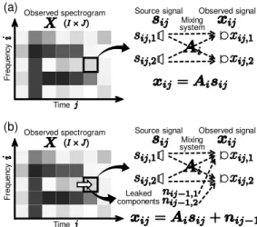
Frequency

Time Observed spectrogram

(a) Source signal

Mixing system

Observed signal

Source signal Mixing system

Observed signal

Frequency

Time Observed spectrogram

Leaked components

(b)

Fig. 1. Mixing system of each spectrogram slot when N = M = 2; (a) has a linear time-invariant mixing system and there is no reverberation; (b) has some leaked components from the previous frame because of reverberation.

Figure 1 (a) shows the mixing system corresponding to (4). In linear time-invariant mixing, all the time frames are independent of other time frames, meaning that they do not affect each other. However, for the case of reverberant recording, reverberant components can leak from the previous frame as shown in Fig. 1 (b), and the mixed signal xi j cannot be represented using only Ai. Therefore, the assumption of linear time-invariant mixing holds only when the lengths of all impulse responses between the sources and microphones are sufficiently shorter than the length of the window function in the short-time Fourier transform (STFT).

When the assumption is valid and M = N, the estimated source yi j can be represented by a demixing matrix Wi = (wi,1· · ·wi,N)^H(wi,ndenote demixing filters) as

yi j=Wixi j^, (5) where^Hdenotes a Hermitian transpose.

2.2. Principal component analysis for overdetermined BSS

When M > N, in a typical separation method using FDICA or IVA, principal component analysis (PCA) is applied in ad- vance and the dimension of xi jis reduced so that M = N. This preprocessing is performed with the expectation that the reverberant components in the observed signal are eliminated by the dimensionality reduction. Therefore, PCA is applied to make the assumption of linear time-invariant mixing valid even in a reverberant environment. However, if the purpose of source separation is to obtain each source image including the reverberation, PCA degrades the separation performance by removing the reverberation components. Moreover, if the source powers in mixtures are unbalanced (e.g., music signals), PCA can even remove direct components of weak sources, which leads to a greater risk of poor separation.

The assumption of linear time-invariant mixing is made valid by using a sufficiently long window function in the STFT. However, if we use a too long window function for FDICA or IVA, the independence assumption collapses in each frequency band [11]. Therefore, the separation performance has a trade-off based on the length of the window function in terms of the assumptions of linear time-invariant mixing and the independence of sources.

2.3. MNMF with rank-1 spatial constraint

In MNMF [8], the decomposition model of an observed signal Xi j=xi jx^H_{i j}is represented as

Xi j≃ ˆ_Xi j=^∑_k^(∑_n_Hi,nznk) tikvk j, (6) where k = 1, . . . , K is the integral index of the NMF bases (spectral patterns),Hi,nis an M × M spatial covariance matrix for frequency i and source n, znk (∈ R[0, 1]) is a latent variable that clusters K bases into N sources and satisfies^∑n^znk=1, and tik(∈ R≥0) and vk j (∈ R≥0) are the elements of the basis matrix T (∈ R^I×K≥0 ) and activation matrix V (∈ R^K×J≥0 ^{), respec-}

tively. MNMF estimates the spatial covariance matrixH corresponding to each source and the source components T V . The estimated source y is obtained by clustering T V intoH using cluster indicator Z (∈ R^N×K[0, 1]). The variablesH, Z, T , and V are estimated by minimizing the divergence between Xi j and ˆXi j [8]. However, this optimization has a high computational cost, and the separation results strongly depend on the initial values.

As an efficient optimization method for MNMF, Rank-1 MNMF has been proposed [10]. In this method, we assume an overdetermined case, M ≥ N, and the spatial covariance Hi,nis approximated by a rank-1 matrix. This approximation corresponds to the assumption of linear time-invariant mixing. Rank-1 MNMF can estimate the demixing matrix Wi

using fast IVA update rules [12] and the NMF variables T and V using simple NMF update rules. When N = M, the fast update rules of IVA are obtained as [12]

Vi,n= J⁻¹^∑_j⁽^∑_ltil,nvl j,n

)−1

xi jx^H_{i j}, ₍₇₎ wi,n← (WiVi,n⁾⁻¹en^, (8) wi,n←wi,n

(w^H_i,nVi,nwi,n

)−¹₂

, ₍₉₎

yi j,n=w^H_i,nxi j, (10)

where en denotes the unit vector with the nth element equal to unity. The update rules of NMF are obtained as

til,n←til,n

vu uu

t^∑_j_|y_{i j,n}_|²_v_{l j,n}⁽^∑_l_′_t_il′_,n_v_l′_j,n

)−2

∑

j^vl j,n

(_∑

l^′^til^′,nvl^′j,n

)−1 ^, ⁽¹¹⁾

vl j,n←vl j,n

vu uu

t^∑_i_|y_{i j,n}_|²_t_il,n (_∑

l^′^til^′,nvl^′j,n

)−2

∑

i^til,n

(_∑

l^′^til^′,n^vl^′j,n

)−1 ^, ⁽¹²⁾

(3)

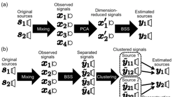
(b) Original sources

Observed signals

Estimated sources PCA

Mixing BSS

Dimension- reduced signals (a)

Original sources

Observed signals

Mixing

Clustered signals Estimated

sources

Reconstruction BSS

Separated signals

Clustering Source 1

Source 2

Fig. 2. Algorithms of (a) conventional and (b) proposed methods (N = 2, M = 4, P = 2).

where l = 1, . . . , L is the integral index of the NMF bases for each source, and til,nand vl j,nare the basis and its activation that represent only source n, respectively. Similarly to (6), we can extend Rank-1 MNMF so that the bases for each source are adaptively determined by the latent variable Z [10].

In Rank-1 MNMF, we can optimize all the variables Wi, T , and V faster and more robustly than in conventional MNMF. However, if the reverberation time of the recorded environment increases, the separation performance markedly degrades because the approximation of the rank-1 spatial model collapses. Conventional MNMF can achieve a certain level of separation even for reverberant signals because this method can estimate full-rank spatial covariance matrixHi,n.

3. PROPOSED METHOD

3.1. Relaxation of rank-1 spatial constraint utilizing extra observations

To relax the constraint of the rank-1 spatial model in Rank- 1 MNMF, we propose the utilization of extra observations for modeling the reverberant components. In this method, we consider that the number of observations M is P times the number of sources N, namely, M = PN. In conventional overdetermined BSS, PCA is applied before the separation so that M equals N as shown in Fig. 2 (a). In the proposed algorithm, we estimate M separated signalsy as shown in Fig. 2_˜ (b). In this approach, the leaked component from previous frames (ni j−1 in Fig. 1 (b)) of each source is modeled as an additional new source, namely, each original source is represented with rank-P spatial model. To obtain an estimate of the source including both direct and reverberant components, the separated signals must be clustered using some criteria, which is a kind of permutation problem. The clustered separated signaly is represented as follows:_˜

˜ yi j⁼

(˜yi j,11 ^{· · ·} ˜yi j,1P ˜yi j,21 ^{· · ·} ˜yi j,2P ^{· · ·} ˜yi j,NP

)T

, (13)

yi j,n=^∑_p˜yi j,np^, (14)

where ˜yi j,n1^{, . . . ,}˜yi j,nPcorrespond to the direct and reverberant components of one source n. Finally, each estimated source yi j,nis reconstructed by summing of the clustered components as represented by (14).

3.2. Clustering with spectral correlations

In Sect 3.1, the complex-valued spectrograms of the sources are estimated by assuming the independence between them. However, we can expect that the power spectrograms of the direct and the reverberant components for the same source have a correlation. Based on this assumption, we propose to use cross-correlation between the power spectrograms ˜Y_{i j,np}=

|˜yi j,np^|²to determine which separated signal ˜yi j,npcorresponds to the direct or reverberant component of which source:

C(A∥B) = max^({^∑i, j^ai j^bi j+τ^{| τ =}0, 1, . . . , τmax

}) , (15) where A (∈ R^I×J≥0) and B (∈ R≥^I×J0) are the power spectrograms, ai jand bi jdenote the elements of A and B, respectively, and τis an index of the delay in the time frame. For clustering, we first calculate (15) between all separated signals ˜yi j,np. Then, the signals are merged in descending order of C until the number of clusters becomes N, with all the clusters (signal sets) required to have the same number of signals (see Fig. 3). 3.3. Auto-clustering with basis-shared Rank-1 MNMF For Rank-1 MNMF, we can consider another approach for clustering the signals ˜yi j,np. Since the reverberation consists of a sum of time-delayed versions of the direct component, it is represented by the convolution. Even in the power spectrogram domain, this model is approximately valid [13]. If we assume that the impulse response in the power spectrogram domain is identical over all frequency bins, the direct and reverberant components of the same source can be modeled by the same bases Tn(spectral patterns) and different activations Vnp(time-varying gains) as follows:

Yñ1 ≃TnVn1^, Y^ñ2≃TnVn2^, ^{. . . ,} Y^ñP≃TnVnP^, (16) where ˜Ynp(∈ RÎ×J_≥0) is the power spectrogram of signal ˜yi j,np, Tn (∈ RÎ×L≥0) is a shared basis matrix whose elements are ti1,n, . . . ,tiL,n, and Vnp (∈ R^L×J≥0) is an activation matrix whose elements are v1 j,np^{, . . . ,}vL j,np. This basis sharing leads to the separated signals ˜yi j,n1^{, . . . ,}˜yi j,nP representing the direct and reverberant components of one source n. The cost function of basis-shared Rank-1 MNMF can be defined as

Q =^∑_{i, j} [

∑

n,p

|˜yi j,np^|²

∑

l^til,nvl j,np

−2 log | det Wi| +^∑_n,plog^∑l^til,nvl j,np

]

. ₍₁₇₎ The update rules of Wifor minimizing (17) are the same as (7)–(10) if we consider N ← M = NP, and the update rules of the NMF variables are obtained as follows:

til,n←til,n

vu uu

t^∑_j,p_|y_{i j,np}_|²_v_{l j,np}⁽^∑_l_′_t_il′_,n_v_l′_j,np

)−2

∑

j,p^vl j,np

(_∑

l^′^til^′,nvl^′j,np

)−1 ^, ⁽¹⁸⁾

vl j,np←vl j,np

vu uu

t^∑_i_|y_{i j,np}_|²_t_il,n (_∑

l^′^til^′,nvl^′j,np

)−2

∑

i^til,n

(_∑

l^′^til^′,n^vl^′j,np

)−1 ^. ⁽¹⁹⁾

(4)

Sort in descending order.

1. 2. 3. 4.

Merge and as a set . already has two components. (do not merge into )

Merge and as a set . already has two components. (do not merge into ) Calculate for all

combinations of spectrograms .

Cluster the signals .

Fig. 3. Hierarchical clustering using correlation C (N = 2, M = 4, P = 2), where all sets must have the same number of signals.

Reverberation time: 470 ms

2 m Source 1

80 JR2 impulse

response from RWCP database

60 Microphone

interval: 2.83 cm

Source 2

Fig. 4. Recording conditions of room impulse response. However, the clustering result fluctuates depending on the initial values of the variables. To avoid this problem, we used IVA and the clustering method described in Sect 3.2 to obtain initial value of demixing matrix Wi.

4. EXPERIMENT 4.1. Conditions

To confirm the efficacy of the proposed algorithm, we con- ducted an evaluation experiment using professional music signals. In this experiment, we produced observed signals with M = 4 channels and N = 2 sources by convoluting the impulse response JR2 (see Fig. 4) from the RWCP database [14] with each source. Table 1 shows the songs and sources used, which were obtained from SiSEC [15]. We compared IVA with PCA (PCA+IVA) and Rank-1 MNMF with PCA (PCA+Rank-1 MNMF), which both assume the rank-1 spatial constraint. In addition, two types of conventional MNMF [8] were also evaluated: MNMF w/o MWF and MNMF+MWF. In MNMF w/o MWF, the maximum SNR beamformer [16], which is calculated from the estimated spatial covarianceHi,n, was used for separation. MNMF+MWF utilizes multichannel Wiener filtering (MWF) to enhance the estimated sources. As the proposed methods, constraint-relaxed IVA with the clustering method in Sect. 3.2 (Proposed IVA) and constraint- relaxed Rank-1 MNMF with basis sharing (Proposed Rank-1 MNMF) were evaluated, where the pretrained and clustered demixing matrix was used for the initial value in Proposed Rank-1 MNMF. Moreover, we evaluated the limit separation performance of linear filtering (Ideal linear filter), which is the maximum SNR beamformer calculated using the ideal spatial covariances of each source. It is necessary to apply a back-projection technique [17], except for in MNMF+MWF, to the estimated sources. The characteristics of each method are shown in Table 2 and the other conditions are described in Table 3. Note that we used a 128-ms-long window in the STFT for the signals that have 470-ms-long reverberation,

Table 1. Music sources

ID Song Source (1/2)

1 bearlin-roads snip 85 99 acoustic guit main/piano 2 fort minor-remember the name snip 54 78 drums/vocals 3 ultimate nz tour snip 43 61 guitar/vocals

Table 2. Characteristics of each method

Method # of filters per source Postfilter

PCA+IVA 1 None

PCA+Rank-1 MNMF 1 None

MNMF w/o MWF 1 None

MNMF+MWF 1 MWF

Ideal linear filter 1 None

Proposed IVA 2 None

Proposed Rank-1 MNMF 2 None

which means that the rank-1 spatial model collapses. As the evaluation scores, we used the signal-to-distortion ratio (SDR) [18], which indicates the total separation performance. 4.2. Results

Figure 5 shows the average scores and their deviations in 10 trials with various initializations. The methods using PCA cannot achieve good separation because they require the rank- 1 spatial approximation. The scores of MNMF w/o MWF indicate poor separation accuracy and strong dependence on the initial values because it is difficult to estimate the full- rank spatial covarianceH. However, MWF with NMF variables can greatly enhance the estimated sources. Proposed Rank-1 MNMF separates the sources with high accuracy. In particular, this method outperforms the limit performance of linear filtering (Ideal linear filter) as shown in Figs. 5 (b) and (c). This is because ground truth sources include reverbera- tions, which can span more than two dimensional space, and the proposed algorithm can effectively relax the rank-1 spatial constraint. Table 4 shows actual computational times for the separation of song ID3, where the calculations were performed using MATLAB 8.3 (64-bit) with an Intel Core i7- 4790 (3.60 GHz) CPU. The computational time of Proposed Rank-1 MNMF includes the initialization time for Wi, which is the same as that of Proposed IVA. We confirm that Pro- posed Rank-1 MNMF can maintain efficient optimization and achieve good separation performance.

5. CONCLUSION

In this paper, we proposed a new relaxation method for the rank-1 spatial constraint. This method utilizes extra observations to estimate reverberant components while maintaining the rank-1 model. The efficacy of the proposed method was confirmed with IVA and Rank-1 MNMF, and they achieved a good separation performance even for reverberant signals.

REFERENCES

[1] P. Comon, “Independent component analysis, a new concept?,” Signal Processing, vol.36, no.3, pp.287– 314, 1994.

(5)

Table 3. Experimental conditions

Sampling frequency Downsampled from 44.1 kHz to 16 kHz

FFT length 128 ms

Window shift 64 ms

Number of bases L =15 (K = 30)

Maximum delay in time frame τ_max=2

Number of iterations 200

12 10 8 6 4 2 0 -2 ]eB[dt nemvSropm iRD -4

Source 1 Source 2

(b)

PCA+IVA PCA+Rank1

MNMF w/o MWF^MNMF ^MNMF+MWF linear filter^Ideal ^ProposedIVA Rank-1 MNMF^Proposed

16 14 12 10 8 6 4 2 ]eB[dt nemvSropm iRD 0

Source 1 Source 2

(c)

PCA+IVA PCA+Rank1

12 10 8 6 4 2 0 -2 ]eB[dt nemvSropm iRD -4

Source 1 Source 2 PCA+IVA PCA+Rank1

(a)

Fig. 5. Average SDR improvements for (a) song ID1, (b) song ID2, and (c) song ID3.

Table 4. Computational times for separation of song ID3 (s)

PCA+IVA ^PCA+Rank-1 MNMF+MWF ^Proposed ^Proposed

MNMF IVA Rank-1 MNMF

23.4 29.4 3611.8 60.1 143.9

[2] P. Smaragdis, “Blind separation of convolved mixtures in the frequency domain,” Neurocomputing, vol.22, pp.21–34, 1998.

[3] H. Saruwatari, T. Kawamura, T. Nishikawa, A. Lee and K. Shikano, “Blind source separation based on a fast-convergence algorithm combining ICA and beam- forming,” IEEE Trans. ASLP, vol.14, no.2, pp.666–678, 2006.

[4] D. D. Lee and H. S. Seung, “Algorithms for nonnegative matrix factorization,” Proc. NIPS, vol.13, pp.556–562, 2001.

[5] S. Makino, T.-W. Lee and H. Sawada, “Blind Speech Separation,” Springer, 2007.

[6] H. Kameoka, M. Nakano, K. Ochiai, Y. Imoto,

K. Kashino and S. Sagayama, “Constrained and regu- larized variants of non-negative matrix factorization in- corporating music-specific constraints,” Proc. ICASSP, pp.5365–5368, 2012.

[7] A. Ozerov and C. F´evotte, “Multichannel nonnegative matrix factorization in convolutive mixtures for audio source separation,” IEEE Trans. ASLP, vol.18, no.3, pp.550–563, 2010.

[8] H. Sawada, H. Kameoka, S. Araki and N. Ueda, “Multi- channel extensions of non-negative matrix factorization with complex-valued data,” IEEE Trans. ASLP, vol.21, no.5, pp.971–982, 2013.

[9] T. Kim, H. T. Attias, S.-Y. Lee and T.-W. Lee, “Blind source separation exploiting higher-order frequency de- pendencies,” IEEE Trans. ASLP, vol.15, no.1, pp.70– 79, 2007.

[10] D. Kitamura, N. Ono, H. Sawada, K. Kameoka and H. Saruwatari, “Efficient multichannel nonnegative matrix factorization exploiting rank-1 spatial model,” Proc. ICASSP, pp.276–280, 2015.

[11] S. Araki, R. Mukai, S. Makino, T. Nishikawa and H. Saruwatari, “The fundamental limitation of frequency domain blind source separation for convolutive mixtures of speech,” IEEE Trans. SAP, vol.11, no.2, pp.109–116, 2003.

[12] N. Ono, “Stable and fast update rules for independent vector analysis based on auxiliary function technique,” Proc. WASPAA, pp.189–192, 2011.

[13] H. Kameoka, T. Nakatani and T. Yoshioka, “Robust speech dereverberation based on non-negativity and sparse nature of speech spectrograms,” Proc. ICASSP, pp.45–48, 2009.

[14] S. Nakamura, K. Hiyane, F. Asano, T. Nishiura and T. Yamada, “Acoustical sound database in real envi- ronments for sound scene understanding and hands-free speech recognition,” Proc. LREC, pp.965–968, 2000. [15] S. Araki, F. Nesta, E. Vincent, Z. Koldovsk´y, G. Nolte,

A. Ziehe and A. Benichoux, “The 2011 signal separation evaluation campaign (SiSEC2011):-audio source separation,” Proc. LVA/SS, pp.414–422, 2012.

[16] H. L. Van Trees, “Detection, Estimation, and Modula- tion Theory, Optimum Array Processing (Part IV),” Wi- ley Interscience, 2002.

[17] N. Murata, S. Ikeda and A. Ziehe, “An approach to blind source separation based on temporal structure of speech signals,” Neurocomputing, vol.41, no.1–4, pp.1– 24, 2001.

[18] E. Vincent, R. Gribonval and C. F´evotte, “Performance measurement in blind audio source separation,” IEEE Trans. ASLP, vol.14, no.4, pp.1462–1469, 2006.