Study of Feature Extraction for
Motor-Imagery EEG Signals
Hiroshi Higashi
DISSERTATION
Submitted to The Graduate School of Engineering of Tokyo University of Agriculture and Technology
in Electronic and Information Engineering for The Degree of
DOCTOR OF PHILOSOPHY
TOKYO UNIVERSITY OF AGRICULTURE AND TECHNOLOGY December 2013
Abstract
This study proposes signal processing methods to presume or classify brain state of a human by using signals observed by electrodes installed on a scalp (EEG; Electroencephalogram). The issue of classifying the brain states from EEG signals is important for realization of brain computer/machine interface (BCI/BMI) and its applications (e.g. rehabilitation). Target states of the brain to be classified in the study are brain states when the human is imaging movements of he/she own hands and feet. The task performing the imaginations is called motor-imagery (MI) task. The goal in this classification is to classify EEG signals into classes corresponding to motor-imagery parts of body (e.g. right/left hand, feet)
As features in the EEG signals associated with the MI tasks, the variation in energy of certain bands observed around motor cortex is known. For extracting the features, we can use a spatial filter that weights with different coefficients to each electrode, a frequency filter that extracts the certain bands, and a time window that removes periods not including feature components. In many cases, the parameters such as the coefficients of the filters and the window are empirically determined based on knowledge of neuroscience. For instance, the electrodes are installed around motor cortex, the passband of the frequency filter is set to 7 to 30 Hz including the band of the so-called mu rhythm the energy of which decrease by MI tasks, and the time window extracts signals observed from a start cue having
i
a subject perform a task to an end cue. However, the optimal parameters for the filters highly depend on measurement environments and individuals. Therefore, a decision method for the parameters adapted for data is needed.
This study proposes methods to determine the parameters by learning ob- served samples. The proposed methods expand the concept of the common spatial patterns (CSP) method that is well-known for designing effective spatial filters for classification in 2-class MI-BCI. The proposed methods extract a signal from a raw observed signal by the following way. First, we adopt an FIR filter as the frequency filter. Second, we use linear combination of a multi-channel signal and weight coefficients as the spatial filter. Finally, we apply a time window with binary coefficients to a signal after the start cue. To determine the parameters composed of three elements (frequency, space, time), we take advantage of EEG signals with class labels as a learning dataset. In the learning, the parameters are determined in such a way that the ratio of the energy of the extracted signals between two classes is maximized. We propose an approximate solution using a method that maximizes alternately parameters of each element. Moreover, we introduce an orthogonal constraint over the coefficient vectors of the multiple FIR filters. We propose a sequentially optimizing method for the optimization problem including the orthogonal constraint. In this way, the proposed method designs a set of the filters (filterbank) that have different characteristics in each other. Even in the situation that some components are associated with the MI task, the proposed method is able to extract separately the components by the use of the filterbank.
Moreover, collecting EEG signals takes a long time and small sample prob- lem in the parameter learning can happen. It causes overfittings and ill-posed problems. To address the problem, we propose regularizations for optimization
iii problems of the spatial filters. At first, we make an assumption that the electrodes that are located close to each other observe an electric activity of the same neu- rons. Under the assumption, the proposed regularizations work in such a way that the weight coefficients or the weighted signals for the nearby sensors take similar values in the optimization problems. By adding spatial information of an electrode arrangement as a prior information, the robust coefficients of the spatial filter can be found.
Experimental analysis for the proposed methods is conducted with artificial signals. Moreover, we show the EEG classification experiments of the MI tasks. The results show the proposed methods improve accuracy of the classification.
Acknowledgements
This work would not have been possible without the guidance of my academic supervisor, Dr. Tohihisa Tanaka. I am very grateful for his advice and support that have opened new gates of opportunities. My deepest gratitude also goes to the doctoral committee members, Dr. Hitoshi Kitazawa, Dr. Masatoshi Sekine, Dr. Akinobu Shimizu, and Dr. Toshiyuki Kondo. Their questions, comments, and suggestions have greatly helped in the improvement of this work.
I would like to extend my grateful acknowledgement to the Japan Society for the Promotion of Science (JSPS) and RIKEN. They have helped me with financial support throughout my academic life.
I would like to thank to Dr. Cichocki Andrzej, the head of the Laboratory for Advanced Brain Signal Processing, Brain Science Institute, RIKEN, and members of his laboratory. He has given me opportunities for collaborations with his lab- oratory. Especially, I am grateful to ex-researchers in the laboratory, Dr. Tomasz M. Rutkowski who is now an assistant professor, The University of Tsukuba, and Dr. Yoshikazu Washizawa, who is now an assistant professor, The University of Electro-Communications.
I would like to represent gratitude to the Machine Learning Group, Berlin Institute of Technology. Dr. Klaus-Robert M¨uller, the head of the group, and Dr. Benjamin Blankertz accepted my request to stay in their laboratory for three
v
months. The members of the laboratory gave me useful advices and showed some advanced researches that encourage me to study hard. The experience in Berlin made me grow up as a researcher.
I am grateful for professors and fellows who have given me valuable advices at conferences. To the members of Toshihisa Tanaka’s laboratory, I would like to thank for a good time with you and your valuable supports.
Last, thank my family. I am very grateful to your financial and moral supports to me.
Contents
1 Introduction 1
1.1 Background . . . 1
1.2 Problems . . . 5
1.3 Solutions . . . 6
1.4 Organization of Thesis . . . 10
1.5 List of Symbols . . . 11
2 EEG-Based Brain Machine Interfaces 13 2.1 Fundamentals of Brain Machine Interfaces . . . 13
2.2 Methods for Measuring Brain Activity . . . 16
2.2.1 Functional Magnetic Resonance Imaging . . . 16
2.2.2 Near-Infrared Spectroscopy . . . 16
2.2.3 Magnetoencephalography . . . 17
2.2.4 Electroencephalography . . . 17
2.3 Variety of EEG-based Brain Machine Interfaces . . . 20
2.3.1 Perception of Random-Displayed Stimuli . . . 20
2.3.2 Gazing at Flicker Stimuli . . . 23
2.3.3 Imagination of Muscle Movements . . . 26 vii
3 Feature Extraction for Motor-Imagery EEG 31
3.1 Features Associated with Motor-Imagery Task . . . 31
3.2 Discrete Fourier Transform . . . 32
3.3 Common Spatial Pattern . . . 33
3.4 Common Spatio-Spectral Pattern . . . 35
3.5 Common Sparse Spectral Spatial Pattern . . . 36
3.6 Spectrally Weighted CSP . . . 37
3.7 Filter Bank Common Spatial Patterns . . . 39
4 Common Spatio-Time-Frequency Patterns 41 4.1 Signal Extraction Model . . . 42
4.2 Optimization for Sets of Parameters . . . 43
4.3 Feature Vector Definition . . . 48
4.4 Convergence of Cost Function in Optimization . . . 48
4.5 Search Space for FIR Filter Coefficients . . . 49
4.5.1 Subspace Spanned by Filter Coefficients Vectors . . . 49
4.5.2 Subspace Spanned by Filter Coefficients Vectors and Its Shifted Vectors . . . 49
4.6 Simulation by Artificial Signal . . . 50
4.7 Classification Experiment of BMI Datasets . . . 56
4.7.1 Data Description . . . 58
4.7.2 Result . . . 59
4.8 Conclusion . . . 66
5 Regularization with Sensor Positions 73 5.1 Distance Between Electrodes . . . 73
CONTENTS ix
5.2 Regularization . . . 75
5.3 CSP with Regularization with Sensor Positions . . . 76
5.4 Simulation by Artificial Signals . . . 77
5.5 Classification Experiment of BMI Datasets . . . 78
5.5.1 Data Description . . . 78
5.5.2 Features for Classification . . . 79
5.5.3 Results . . . 79
5.6 Conclusion . . . 82
6 Conclusions and Open Problems 87 6.1 Conclusions . . . 87
6.2 Open Problems . . . 88
6.2.1 Adaptive System for Unstationary Feature Components . . 89
6.2.2 Application to Self-Paced BMIs . . . 89
6.2.3 Application to Rehabilitation . . . 90
A Proofs 109 A.1 Proof of Theorem 1 . . . 109
A.2 Proof of Proposition 1 . . . 111
B List of Publications 113
List of Tables
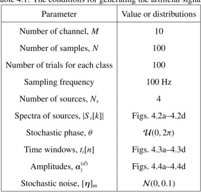
4.1 Conditions for generating artificial signals . . . 52 4.2 Description of the datasets. . . 57 4.3 Parameters decided by nested CV . . . 62 4.4 Classification accuracy rates given by 5×5 CV in dataset IVa from
BCI competition III . . . 63 4.5 Classification accuracy rates given by 5×5 CV in dataset 1 from
BCI competition IV . . . 64 4.6 Classification accuracy rates given by 5×5 CV in original dataset . 65 5.1 The settings for generating artificial signals . . . 78 5.2 Classification accuracy rates given by 100 training samples . . . . 81 5.3 Classification accuracy rates given by 5 training samples . . . 82
xi
List of Figures
2.1 Fundamental structure of BMI . . . 14
2.2 Electrode arrangement of International 10-20 method and Inter- national 10-10 method . . . 18
2.3 Waveform of P300 . . . 21
2.4 Interface of BMI system making telephone call . . . 22
2.5 Procedure for stimuli in telephone call BMI . . . 23
2.6 Power spectrum of signals observed when subject gazes at flicker stimulus. . . 25
2.7 Interface for SSVEP-based BMI . . . 26
2.8 Monochrome inversion in checkerboard . . . 27
2.9 ERD by motor imagery tasks of left and right hand . . . 28
3.1 Sensory and motor cortex and associated body regions . . . 32
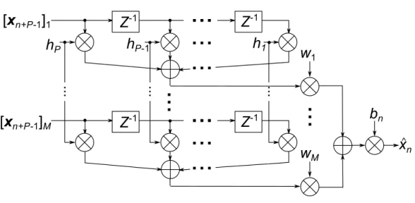
4.1 Signal extraction with temporal filter, spatial weights, and time window . . . 42
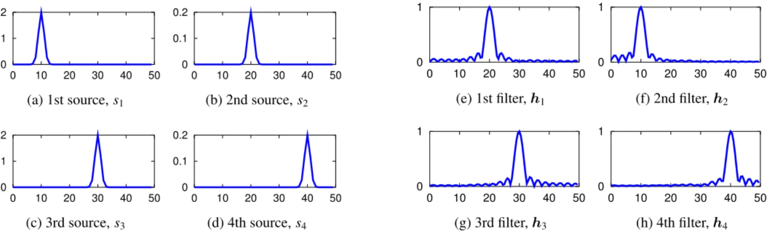
4.2 Frequency patterns of sources and frequency filters . . . 53
4.3 Time patterns of sources and time window . . . 54
4.4 Spatial patterns of sources and spatial weights . . . 55 xiii
4.5 Variation of accuracy rates by various T1in CSP . . . 66
4.6 Variation of accuracy rates by various T1in each method . . . 67
4.7 Variation of accuracy rates by various regularization parameters in BCI competition III dataset IVa . . . 68
4.8 Variation of accuracy rates by various regularization parameters in BCI competition IV dataset 1. . . 69
4.9 Examples of spatio-time-frequency patterns in subject aa . . . . . 70
4.10 Examples of spatio-time-frequency patterns in subject av . . . . . 71
5.1 3-dimensional plot of International 10-20 method . . . 74
5.2 Source signals in artificial signal . . . 79
5.3 Spectrum of source signals in artificial signals . . . 80
5.4 Spatial distributions of source signals in artificial signals . . . 81
5.5 Examples of observed signals in artificial signals . . . 82
5.6 Topographical maps of spatial weights in experiment of artificial signals . . . 83
5.7 Topographical maps of the spatial weights for subject ay . . . . . 84
Chapter 1
Introduction
1.1 Background
Decording brain activity from brain signal is an important and challenging tech- nology. The applications of the technology are detection of diseases [1, 2], design of an interface [3] and research for brain function [4–7], etc. An interface us- ing brain signal is called a brain machine interface (BMI). BMI is an interface connecting a human brain and an external device. Especially, BMIs to send com- mands to the device is called output-type BMIs. A brain activity that is evoked by certain tasks is allocated to an output of the interface. A user of the interface performs the allocated tasks to generate the output. The tasks inducing the brain activities are not limited to just tasks with muscular movements. Certain mental tasks such as turning attention to external stimuli and imagination of something can be used as the tasks for BMIs. Therefore BMIs realize non-muscular com- munication and control channel for conveying messages and commands to the external world [3, 8, 9].
BMI is a challenging technology of nueroscience, signal processing, and pat- 1
tern recognition. From the neuroscience point of view, they explore mental tasks and responses to stimuli that can be observed in brain signals. People who are in signal processing and pattern recognition societies are interested in how to extract the features evoked by the tasks from the observed signals and how to classify the extracted features to the task. Above all, this study mainly tackles problems of how to extract features associated to the tasks.
For acquisition of the brain signals in BMI, there are invasive and noninvasive methods [10]. Electrocorticogram (ECoG), electrosubcorticogram (ESCoG), and electroventriculogram (EVG) are typical invasive measurement methods. They need surgeries for installing electrodes on a cortex or a cerebral ventricle and measure electrical activities of brain neurons. The invasive methods can measure the brain activities with noise much less than that in the noninvasive methods. BMIs with the invasive measurements have realized without muscle movements a control of a lever by a rat [11], a control of a robot arm by a monkey [12], and a control of a computer cursor by a patient suffering from motor disorders [13]. On the other hand, the noninvasive methods do not require such medical surg- eries. The noninvasive methods are considered that they impose a less load on subject and are more practical methods for realizing BMIs than the invasive meth- ods [14]. Noninvasively measured data such as electroencephalogram (EEG) [15], magnetoencephalogram (MEG) [16], and functional magnetic resonance imag- ing (fMRI) [17], and near-infrared spectroscopy [18] are widely used to the BMI research. The details of these noninvasive methods are shown in Chapter 2.2. Among them, because of its simplicity and low cost, EEG is practical for use in engineering applications [19, 20]. Moreover, EEG can achieve higher temporal resolution than the other invasive methods [8]. In this study, we use EEG as the
1.1. BACKGROUND 3 measurement method for BMI. Although EEG is considered to be practical for BMI, decrease of desired components, high noise, and low spatial resolution are significant problems. The BMI systems with EEG (EEG-based BMI) such as an input of letters [21–23] and controls of an object in a monitor [24, 25], a wheel chair [26], and a robot [19, 27] have been developed.
BMIs can be categorized by the tasks which a subject performs. The frame- works composed of the tasks and feedbacks to the subject are often called paradigms. Typical BMI paradigms are perception of random-displayed stimuli, gazing at flicker stimuli, and imagination of muscle movements. The details of these paradigms are shown in Chapter 2.3. This paradigm of imagination of muscle movements is called the motor-imagery (MI) paradigm and the BMI using MI is called MI- based BMI (MI-BMI) [3, 9]. In MI-BMI, an observed brain signal is classified into classes corresponding to a body part which a subject imagines movement of. For example, the right hand, the left hand, feet, and tongue of the MI tasks are widely used for realizing BMI [28, 29].
This study addresses problems for feature extraction in the BMI using the paradigm of imagination of muscle movements. The reasons why we focus on the MI paradigm are as follows. As merits as an interface, unlike the paradigms that make use of responses to some stimuli, MI-BMIs do not need stimuli because a subject performs the MI tasks voluntarily. Moreover, the subject needs at least a perception out of visual, auditory, tactile, olfactory, and gustatory perceptions in order to respond to the stimuli. On the other hand, the MI paradigm can be used by patients suffering from sense disorders and even for locked-in patients. Re- cently, some researches explore a new field of application of MI-BMI in medical rehabilitation area [30, 31]. The rehabilitation of the application aims to recover
motor function in patients who have damages in brain regions that play a role in the motor function. Typically, the rehabilitation asks the patient to try to move its paralyzed limb. Then, the motor function can be gradually recovered as the patient tries it repeatedly. The recovery makes use of neuroplasticity that is a property of changes in neural pathways and synapses which are resulted by stimuli such as behavior, environment and neural processes [32]. Thanks to neuroplasticity, the disabled motor function is recovered in the different region from the damaged re- gion. In the process of trying the movement, it has been suggested that physical feedbacks to the paralyzed part promote neuroplasticity [33]. For instance as the feedbacks, a robot gives force to the paralyzed part and moves the part. Some researches suggest that the use of BMI for the control of the feedbacks is effective for promotion of neuroplasticity [31, 34, 35]. BMI is used for detecting patterns of MI or an intention of movements in a brain signal and makes the feedbacks when it the patterns is detected. The feature patterns in the brain signal according to MI and the intention of movement are thought to be similar [36]. As we mentioned, the application areas of MI-BMI are widespread, and classification of brain states of MIs is an important issue in these applications.
Different MI tasks (e.g. imaginations of movements in a left hand, a right hand, feet, and a tongue) evoke different feature patterns in EEG [3, 37]. Espe- cially, the change in energy of a certain frequency band called mu band [8] is well known as a feature related to MI. The mu band is the name of the frequency band of 10–15 Hz in EEG and MEG signals and there are some bands named such as alpha, beta, and theta bands (waves) in brain science [38]. The energy in the mu band observed in a motor cortex decreases while a subject performs the MI tasks. This decrease of the energy is called event related desynchronization (ERD) and
1.2. PROBLEMS 5 the location observing ERD depends on the body part of which a subject imag- ines the movement [8, 39–41]. Extraction of these changes from the measured EEG signals enables us to classify the EEG signal associated with the different MI tasks.
1.2 Problems
For classification of some MI tasks, we have to extract the features in the presence of measurement noise and spontaneous components which are related to the other brain activities because the features, noise and the other components are mixed in the observed EEG signals. For the extraction of the features, signal processing techniques such as bandpass filtering and spatial weighting are used [3]. For the processing, finding the parameters such as coefficients of the filters and weights that accurately extract the related components is a crucial issue. The knowledges in neuroscience have been often used to design the parameters. However, the opti- mum parameters in classification are highly dependent on users and measurement environments [42]. In order to determine the parameters, data-driven techniques that exploit observed data are widely used [3, 8]. The observed data essentially include class labels corresponding to the tasks. The dataset of the data with the class labels refers to a learning dataset in machine learning literacy. The data- driven techniques try to find the parameters that extract discriminative features as much as possible. To this end, it would be simple to apply cross validation (CV) for searching these parameters that give the best classification accuracy for the learning dataset among several candidates of the parameters. However, the clas- sification performance depends on the choice of the candidates and the selected filter is not always “optimal.” Moreover, a large size of the candiate set leads to
high computational cost.
As the data-driven methods, common spatial pattern (CSP) method is widely used for design of the spatial weights in MI-BMIs. The method finds the spatial weights by using the observed signals [3, 42, 43] in such a way that the variances of the signal extracted by the linear combination of a multichannel signal and the spatial weights differ as much as possible between two classes. The standard CSP method has been extended to methods to estimate the other parameters such as the frequency bands [44–49], and methods to select the CSP features extracted with various parameters [50, 51]. The feature extraction procedures in these methods can be modeled by a model applying spatial weights, frequency filters, and time windows to EEG signals.
The study focuses on three problems regarding to the design of the parameters in the model;
1) simultaneous design of spatial weights, frequency filters, and time windows is impossible,
2) extraction of multiple feature components modeled with different spatial patterns, frequency patterns, and time patterns for each other is impossible, 3) overfitting of the designed parameters for the spatial weights often happens.
1.3 Solutions
We propose a method to solve the problems 1) and 2) in Chapter 4 and a method to solve the problem 3) in Chapter 5.
Chapter 4 proposes common spatio-time-frequency patterns (CSTFP). This method is one of the extensions of CSP. The different points from the existing
1.3. SOLUTIONS 7 methods, which design the spatial weights and frequency filters, are that CSTFP can simultaneously design sets of the spatial filter, the frequency filter, and the time window. The reasons of the importance of design of the sets of the filters are described in the following two paragraphs.
The first reason relates to the problem 1). A kind of BMIs is implemented based on cues which a user follows. In this BMI, the user begins to perform a task when the cue is given. Therefore, the time when the user begins to perform the task is known. However, when the brain activity associated to the task occurs is unknown. The time windows working to remove samples that do not contain the brain activity will not match the period when the cues are showed. For in- stance, the samples for a few hundreds milliseconds after the cues are assumed not to be used to extract the features in previous works [46, 50, 52, 53], which heuristically determined the time window. Contrary to these works, this study hy- pothesizes that an optimal observation period in classification depends on users. For example, reaction time defined as the elapsed time between the presentation of a sensory stimulus and the subsequent behavioral response is strongly associ- ated with age [54]. The reaction time can be related to the time to response to the cues. Therefore, the time window should also be designed by using the observed signals or data-driven.
The second reason relates to the problem 2). It is suggested that the feature components evoked by performing the MI tasks are observed in the mu and beta bands [37]. Therefore, a bandpass filter with a passband of 7–30 Hz including the mu and beta bands is widely used in feature extraction in MI-BMI [42, 43, 55]. These two components in the mu and beta bands are considered to have different frequency bands, different spatial patterns, and different time patterns [3,
9]. Because of the suggestion about the mu and beta bands, we suggest that the features associated to the MI task are in various patterns. Therefore, multiple filter sets that separately extract each patterns are needed.
Moreover, the CSTFP method does not have the following problems that the existing methods have. Common spatio-spectral pattern (CSSP) [44] and common sparse spectral spatial pattern (CSSSP) [45] are the methods that obtain coeffi- cients of a finite impulse response (FIR) filter by applying CSP to the combination of observed signals with the time-delayed signals. However, CSSP provides very poor frequency selectivity due to the limitation of a single delay. Unlike CSSP that provides different spectral patterns for each channel, CSSSP can provide a com- mon spectral pattern for all channels. However, CSSSP needs the computationally expensive optimization because the optimization problem for the filter involves a sparsity cost and an extensive parameter tuning is needed. Spectrally weighted CSP (SPEC-CSP) [46] and iterative spatio-spectral patterns learning (ISSPL) [56] use iterative procedures for optimizing spatial weights and a filter, where the spa- tial weights are optimized by CSP and the filter parameterized by weights for the spectrum is found by an optimization problem based on other criteria. These two optimization problems are alternately solved, however this alternating iteration is not guaranteed to be converged, because the cost functions for these two prob- lems are different. Recently proposed sub-band CSP (SBCSP) [57] and filter bank CSP (FBCSP) [50] are based on subband decomposition with multiple filters that have different passbands. As reported in BCI competition III [29] and IV, FBCSP achieves a high classification accuracy. In these methods, EEG signals are de- composed into multiple frequency components and CSP is separately applied for each frequency component. By using multiple filters such as these methods, fea-
1.3. SOLUTIONS 9 tures associated to brain activities such as mu and beta rhythms can be separately extracted. The result of FBCSP suggests that feature extraction using subband de- composition is an effective method to increase classification accuracy of MI-BCI. The methods using frequency decomposition need selection of feature values to achieve accurate classification. In order to select the feature values, the methods based on mutual information have been proposed [50, 51]. The other methods for selecting efficient filters also proposed in [58] and [59]. In these methods, the filters in the filter bank have to be designed in advance and the fixed filter bank is independent of dataset. Although the parameters for the filters such as the passbands that accurately extract the feature components can change by users and measurement environments, the method using the fixed filter bank cannot use the filters optimized for a specific user.
Chapter 5 proposes a regularization method to prevent overfitting in the opti- mization of the spatial weights. The data-driven methods for design of the spatial weights like CSP need a large amount of the learning data. Collecting enough amount of the learning data takes long time and a subject will feel fatigue. There- fore, the optimization can be ill-posed and the optimized parameters can be over- fitting because of limited numbers of the learning data. To prevent overfitting or to solve an ill-posed problem in signal processing and machine learning for learning parameters, regularization is widely used [60, 61]. The regularization for an optimization problem is to add to an original cost function a penalty term which represents additional information such as smoothness or bounds of the vec- tor norm of parameters to be optimized. In this way, the regularization can help design more robust spatial weights against ill-posed problems [53]. We propose a regularization to add information of an EEG electrode arrangement to an opti-
mization problem. The regularization is proposed based on the assumption: the signals measured by the electrodes that are located near each other (the nearby sensors) are similar and also the observed components are similar. To describe the assumption, consider a measurement device of EEG where electrodes installed on scalp observe faint electrical difference. The EEG signal reflects the summation of the synchronous activity of thousands or millions of neurons [9,62]. Therefore, the nearby sensors likely observe activities which are induced from the same neu- rons. For the reason, the spatial filters such as the Laplacian filter that averages the signals observed in the nearby sensors are often used for improving SNR in EEG signal processing [8]. Based on the assumption, we propose the regulariza- tion that works in the optimization problems such that the signals weighted by each coefficient of the spatial weights are similar to each other if these signals are observed in the nearby sensors.
The CSTFP method and the regularization are evaluated in their performances by experiments using artificial signals and BMI datasets in each chapter.
1.4 Organization of Thesis
This thesis is divided into six chapters. In Chapter 1, the background regarding this work, the problems, the ideas of the proposed method is discussed. Chapter 2 introduces the foundation of BMIs. Chapter 3 describes feature components in EEG associated with the MI tasks and some methods to extract these features. We introduce the CSTFP method and its experimental results in Chapter 4. The regularization with information of sensor arrangement is introduced Chapter 5. The study is concluded in Chapter 6.
1.5. LIST OF SYMBOLS 11
1.5 List of Symbols
• R: the set of all real numbers
• C: the set of all complex numbers
• Z: the set of all integers
• An italic letter: a scalar, e.g. x and X
• An italic bold lower-case letter: a scalar, e.g. x
• [·]i: the ith entry of a vector
• An italic bold upper-case letter: a matrix. e.g. X
• [·]i, j: the ith row and the jthe column of a matrix
• ·T: transposes for a vector and a matrix, e.g. xT and XT
• | · |: the absolute value of a scalar, e.g. |x|
• ∥ · ∥p: the p-norm of a vector defined as∥x∥p = !"i=1N |[x]i|p
#1/p
• ∥ · ∥: the l2-norm of a vector
• Span{· · · }: the subspace spanned by vectors
• ⊕: an operator to give the direct sum of two subspaces
• ·⊥: the ortognal complement of a subspace
• δi j: the Kronecker delta defined as 1 for i = j and 0 otherwise
• a mod b: an operator to take a residue of dividing a by b.
• ℜ: an operator to take a real part of a complex number.
• N (m, σ2): a Gaussian distribution with a mean, m, and a variance, σ2
• U(a, b): a uniform distribution whose minimum and maximum values are denoted by a and b, respectively
Chapter 2
EEG-Based Brain Machine
Interfaces
In this chapter, we describe EEG-based brain machine interfaces. We describe fundamental structures of BMI in Sec. 2.1. Section 2.2 lists some methods for measuring brain activities of human. Section 2.3 shows principal paradigms for EEG-based BMI.
2.1 Fundamentals of Brain Machine Interfaces
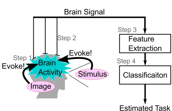
BMIs are interfaces directly connecting brains and external worlds without muscle movements of hands, feet, and a tongue. Figure 2.1 shows a fundamental structure of BMI [9, 14]. As shown in the figure, a procedure of BMI system can be divided into the following four steps.
Step 1 A subject performs certain tasks to induce brain activity in its brain. The certain tasks are mental tasks such as imagination of something or turning attention to a visual/auditory/tactile stimulus.
13
Figure 2.1: A fundamental structure of BMI
Step 2 Brain signal is acquired by measurement systems. Because subsequent signal processing is applied to the digitized signal, the acquired signals are converted to the digital signal by an A/D converter after amplification and filtering are applied.
Step 3 Feature components are extracted from the signal. The signal mixed with components associated to various brain activities and noise are observed. In this step, we remove the noise and extract the components that are associ- ated with the task and are important for the estimation of the tasks.
Both of classical and statistical signal processing techniques (e.g. discrete Fourier transform, FIR/IIR filtering, averaging, principal component analy- sis (PCA), regression analysis, and independent component analysis (ICA)) [63, 64] are used for extracting the feature components. Depending on the tasks,
2.1. FUNDAMENTALS OF BRAIN MACHINE INTERFACES 15 the feature components to be extracted are different. Therefore, we should adopt suitable techniques for this step [8, 65].
Step 4 The task that the subject performs is estimated by recognition of the ex- tracted feature components. The feature components extracted in Step 3 are given as a vector. Hence we can use pattern recognition techniques that are used in the research areas such as speech recognitions and image recog- nition. Classifiers with machine learning (e.g. linear discriminant analy- sis, support vector machine, artificial neural network, and Bayesian classi- fier) [61, 66–68] are widely used for recognizing the tasks with the feature value (vector).
Through these steps, we obtain the task that the subject is performing. The rec- ognized task is used for analysing the subject’s emotions and brain state or is converted to a command to control the device. The BMI system used for inputting the device commands is called an output type of BMI. Because the output type of BMI does not need any muscle movements to send the commands to the devices, the output type of BMI is expected as a communication tool for patients suffer- ing from motor disorders caused by amyotrophic lateral sclerosis, brain stroke, brian or spinal cord injury, cerebral palsy, muscular dystrophies, multiple scle- rosis, and numerous other diseases [9]. BMI is also expected as an interface for virtual reality systems and video games [69]. The application of BMIs spreads to the area of rehabilitation for patients suffering from motor disorders caused by a stroke [30, 31, 33, 70].
2.2 Methods for Measuring Brain Activity
Neurons composing a brain generate spikes (change of electrical potential at short- term) when they accept input stimulus and convey information to the other neu- rons [71]. We capture this kind of changes of electrical potentials and/or blood flows by measurement devices. The information of these changes is used for es- timation of brain state. In this section, we introduce some of the measurement devices. In this study, we focus on EEG with scalp electrodes. This section also shows reasons why we focus on this devices.
2.2.1 Functional Magnetic Resonance Imaging
Functional magnetic resonance imaging (fMRI) is one of neuroimaging proce- dures using magnetic resonance imaging (MRI) [72]. When neuron activates, oxygen is consumed and the blood flow increases in the capillary around the neu- ron [73]. FMRI measures brain activity in the brain or spinal cord of humans or other animals by detecting associated changes in the blood flow.
FMRI is able to obtain high spatial resolution images. However, the change of blood flow is slower than neuron activations and the temporal resolution is poor.
2.2.2 Near-Infrared Spectroscopy
Near-infrared spectroscopy (NIRS) is a spectroscopic method [74]. NIRS uses the near-infrared spectrum (about 800 nm) that reaches inside of a skull through a scalp and a skull. By measuring the reflected light, we can observe the change of amount of hemoglobin and information of exchange of oxygen in the brain.
2.2. METHODS FOR MEASURING BRAIN ACTIVITY 17
2.2.3 Magnetoencephalography
Magnetoencephalography (MEG) is a imaging technique that uses superconduct- ing quantum interference device (SQUID) [75]. SQUID measures magnetic field generated by electrical activities of brain neurons.
2.2.4 Electroencephalography
Electroencephalography (EEG) is a measurement device observing electrical ac- tivity of neuron by using electrodes [76]. The electrical activity that is observed by an electrode is the summation of activities of the group of neurons around the electrode. The electrodes are located on scalp, on cerebral cortex, under cere- bral cortex, and in ventricle and the measurement methods are called scalp EEG, electrocorticography (ECoG), electrosubcorticography (ESCoG), and Electroven- triculography (EVG), respectively. The scalp EEG is an noninvasive measurement method. ECoG, ESCoG, and EVG are invasive measurement methods. This study focuses on the scalp EEG and addresses problems in signal processing for the sig- nal observed by the scalp EEG systems. In the remaining of the thesis, we call the scalp EEG simply EEG unless otherwise specified.
In the EEG measurement, the electrodes are installed on the scalp by using conductivity pastes and special caps. For the BMI application, the EEG signal is usually observed by multiple electrodes [9, 14, 37].In the case of the multi- electrode measurement, International 10-20 [62], Extended 10-20 [77], Interna- tional 10-10 [78], and 10-5 [79, 80] methods have stood as the de-fact standard of the electrode arrangement. In these systems, locations on a head surface are described by relative distances between cranial landmarks over the head surface. For an example, we show how to decide the locations of the electrodes according
Fz
Cz
Pz
Fp1 Fp2
F3 F4
F7 F8
C3 C4
P3 P4
O1 O2
T7 T8
P7 P8
Nz
Fpz
AFz
FCz
CPz
POz
Oz
Iz
F1 F2
F5 F6
F9 F10
FC1 FC2
FC3 FC4
FC5 FC6
FT7 FT8
FT9 FT10
C1 C2
C5 C6
CP1 CP2
CP3 CP4
CP5 CP6
P1 P2
P5 P6
P9 P10
AF3 AF4
AF7 AF8
PO3 PO4
PO7 PO8
T9 T10
TP7 TP8
TP9 TP10
F9 F10
N1 N2
PO9 PO10
I1 I2
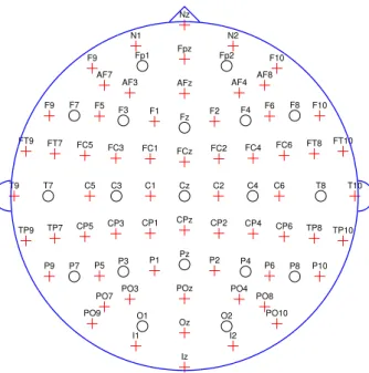
Figure 2.2: The electrode arrangement of the International 10-20 method and the International 10-10 method. The circles show the electrodes defined by the Inter- national 10-20 method. The circles and the crosses show the electrodes defined by the International 10-10 method.
to the International 10-20 method. The landmarks are a nasal point located in the middle point of eyes, the height of eyes, and a inion which is the most prominent point at the back of the head [62]. We drew the line connecting these landmarks along the head surface and moreover make marks that divide the line into short lines of 10% and 20% length of the line. Each electrode point is defined at the intersection point of the lines connecting these marks along the head surface. An examples of the electrode arrangement are shown in Fig. 2.2.
The EEG systems record the electrical potential difference between a two elec- trodes [62]. Referential recording is a method recording the electrical potential difference between a target electrode and a reference electrode and the reference
2.2. METHODS FOR MEASURING BRAIN ACTIVITY 19 electrodes are common to all electrodes. Earlobes that are considered to be elec- trically inactive are widely used as the reference electrode. In contrast, bipolar recording records the electrical potential difference between electrodes located on head surface.
The EEG system can be more compact than the system of fMRI, NIRS, and MRI. Temporal resolution of EEG is higher than fMRI and NIRS [3]. However, it is difficult to make the electrodes for EEG smaller and spatial resolution of EEG is very low comparing with other devices. Moreover, the high frequency compo- nent of electrical activity of neuron decreases in the observed signal because the barriers such as a skull work as a lowpass filter. Additionally, noise caused by poor contacting of the electrode, muscle movements (EMG; electromyography) and eye movements (EOG; electrooculography) contaminates the signal.
The tasks that induce discriminative features in the scalp EEG signal and are available for BMI are limited. The typical tasks for BMI are;
• concentration and meditation,
• perception of random-displayed stimuli,
• gazing at flickering stimulus,
• imagination of muscle movement.
The details of these BMIs are shown in Sec. 2.3.
2.3 Variety of EEG-based Brain Machine Interfaces
2.3.1 Perception of Random-Displayed Stimuli
BMI using perception induces a brain activity called event-related potential (ERP) in a brain by perception to a stimulus. This type of BMIs is widely studied for letter input [3]. The BMI has achieved the input speed of around 1.5 letters per minute [23, 81, 82].
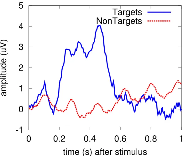
ERPs are electrical changes in EEG signal and they occur when a human per- ceives something. P300 is one of the ERPs. P300 is observed as a positive change of potential after 300 ms from the perception of stimulus [83]. Visual, auditory, tactile, olfactory, and gustatory stimuli are available for inducing P300. An ex- ample of the waveform of P300 is shown in Fig. 2.3. We use the dataset, Dataset II that is an open data in BCI Competition III [28, 84, 85]. The signal labeled
“Targets” is the averaged signal observed in the period 0–1 secs after displaying a stimulus when the subject perceived the stimulus. The signal labeled “Non- Targets” is the averaged signal observed in the period 0–1 sec after displaying a stimulus when the subject does not perceived the stimulus. We can observe the difference of the potentials between “Targets” and “NonTargets” in the period of 0.2–0.4 sec.
In particular, the task called oddball paradigm can induce high potential of P300 [86, 87]. In the oddball paradigm, the subject is asked to react either by counting or by button pressing incidences of target stimuli that are hidden as rare occurrences amongst a series of more common stimuli, that often require no re- sponse. As BMI with the oddball paradigm, BMIs making input of letters have been proposed [3, 88–90]. This kind of BMIs is called P300-spellers. As an
2.3. VARIETY OF EEG-BASED BRAIN MACHINE INTERFACES 21
-1
0
1
2
3
4
5
0 0.2 0.4 0.6 0.8 1
amplitude (uV)
time (s) after stimulus
Targets
NonTargets
Figure 2.3: The waveform of P300. The signals averaged over 85 trials. “Targets” is the observed signal with the subject’s perception after displaying a stimulus.
“NonTargets” is the observed signal without the subject’s perception.
Figure 2.4: An Interface of a BMI system making a telephone call.
example for a BMI using the oddball paradigm, we show an interface of a BMI system making a telephone call. The interface to be presented to a user by a mon- itor is Fig. 2.4. Each row and line flashes during 50–500 ms in random order and the interval between successive flashes is 500 to 1000 ms [89]. The procedure for displaying flash stimuli is illustrated in Fig. 2.5. The user gazes at a target symbol in the interface and counts incidences of the flash of the target symbol. Because P300 happens after 300 ms of the flash of the target, BMI detects whether P300 happens or not for each flash. The BMI decides which symbol the user wants to input.
For detection of P300, recording some trials to input one symbol is often needed due to low signal to noise ratio [88]. Averaging over some trials, low- pass filtering, stepwise linear discriminant analysis (SWLDA) [23, 91, 92] based on linear discriminant analysis (LDA) [61, 93] are used as signal processing for this type of the BMIs.
2.3. VARIETY OF EEG-BASED BRAIN MACHINE INTERFACES 23
Figure 2.5: The procedure for the stimuli in the telephone call BMI. According to the order indicated by the arrows, each row and line flashes.
2.3.2 Gazing at Flicker Stimuli
BMIs using flicker stimuli is an interface where a user inputs a command by gaz- ing at a stimulus flickering at flash frequency of 3–70 Hz [94–96]. This type of BMI does not realize many number of the commands, but achieves higher input speed [3, 14]. However, the flicker stimuli can cause attacks of epilepsy and you should be careful for use [97, 98].
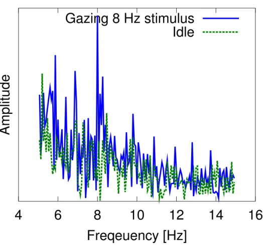
The BMI systems use light emitting diodes (LEDs) [99] or monitors for dis- playing the flicker stimuli [100]. When the subject gazes at the stimuli flickering at 3–70 Hz, steady-state visually evoked potential (SSVEP) is observed in an EEG signal recorded at a visual cortex [98]. Figure 2.6 shows the power spectra of the signals observed when the subject had gazed at the stimuli flickering at 8 Hz for
15 seconds and when the subject had not gazed at it. When the subject gazes at the stimulus, the power spectrum has a peak at 8 Hz. Additionally, there are the other steady state evoked potentials evoked by turning attention to the repeat of a short- term stimulus such as a flicker. The repeat of tactile [101] and auditory [102, 103] stimuli can evoke such potentials.
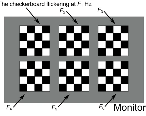
BMI paradigms using SSVEP are as follows. As flicker stimuli, we arrange some checkerboards as in Fig. 2.7 on a monitor. We make monochrome inversion (Fig. 2.8) in the checkerboards at different frequencies for each checkerboard. When the user gazes at the left-top stimulus in Fig. 2.7, SSVEP of F1Hz happens in a recorded EEG signal. By estimating the frequency of SSVEP, BMI decides the stimulus which the user gazes at. Taking a simple way, we can assign the commands to each flicker stimulus and design BMI having six commands with an interface of Fig. 2.7.
The SSVEP-based BMIs have following problems. First, the power of SSVEP is very weak when the flicker frequency is more than 25 Hz [104]. Second, SSVEP of harmonics frequency of a gazed stimulus are also evoked. Therefore, the use of harmonics frequency of a stimulus as the other stimulus frequency can let clas- sification accuracy decrease [100, 105]. Third, in the case of the use of a monitor for displaying the stimuli, available flicker frequencies depend on the refresh rate of the monitor. Due to the above reasons, it is difficult to realize many commands.
To detect SSVEP frequency, discrete Fourier transform can be used. And, canonical correlation analysis (CCA) [106,107] is also widely used for processing for multi-channel EEG signal [108].
2.3. VARIETY OF EEG-BASED BRAIN MACHINE INTERFACES 25
4 6 8 10 12 14 16
Amplitude
Freqeuency [Hz]
Gazing 8 Hz stimulus
Idle
Figure 2.6: The power spectrum of the signals observed when the subject gazes at a flicker stimulus for 15 seconds.
Figure 2.7: An interface for SSVEP-based BMI. Each checkerboard makes monochrome inversion at different frequency.
2.3.3 Imagination of Muscle Movements
BMIs using imagination of muscle movements is an interface where a user inputs a command by imaging movement (motor imagery) of body parts such as hands, feet, and tongue. [3]. This type of BMIs is called the motor-imagery based BMI (MI-BMI). As an example of the MI-BMIs, a task of the motor imagery of right hand and a task of the imagination of the motor imagery of left hand are the tasks to be classified from brain signals.
The tasks of the motor imagery decrease the energy in the certain bands called mu (8–15 Hz) and beta (10–30 Hz) bands in EEG signals observed by the elec-
2.3. VARIETY OF EEG-BASED BRAIN MACHINE INTERFACES 27
Figure 2.8: Monochrome inversion in a checkerboard.
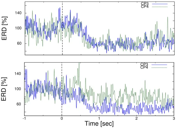
trodes located on (sensory) motor motor cortices. The decrease of the energy is called event related desynchronization (ERD) [8, 39]. Moreover, the location observing ERD depends on the body part of which a subject imagines the move- ment [39–41]. Therefore, we can estimate which body part the subject imagines the movement of from EEG signals by detecting the location where ERD hap- pens. ERD can be observed in not even healthy subject and paralyzed patients. ERD is induced by motor imagery tasks performed by healthy subjects and also paralyzed patients [109]. An example of ERD we can observe in EEG signals is shown in Fig. 2.9. The EEG signals were recorded while a subject performed the tasks of motor imagery of left and right hands [110]. After the recording, the EEG signals that is bandpass filtered with 8–30 Hz. Then these squared signals shown in Fig. 2.9 are averaged over the 100 trials for each motor imagery task of the left or right hand and normalized by a base energy which is averaged over squared signals observed before performing motor imagery tasks. The symbol 0 on the horizontal axis is the time when the subject started performing the tasks. We can observe a decrease in the energy while the subject performs the tasks.
One of the merits of MI-BMI against the BMIs using perception or flicker stimuli is that an instrument for displaying stimuli is unnecessary. Moreover, it
60 100 140
ERD [%]
CP3CP4
60 100 140
-1 0 1 2 3
ERD [%]
Time [sec]
CP3CP4
Figure 2.9: ERD by the motor imagery tasks of left (top) and right (bottom) hands.
2.3. VARIETY OF EEG-BASED BRAIN MACHINE INTERFACES 29 has been reported recently that the detection of the motor imagery tasks and a feedback is useful for rehabilitation for patients who suffer from motor disorders caused by brain damages [30, 31, 33, 70]. MI-BMI will be utilized in the reha- bilitation to recover of the motor functions as follows. One of the rehabilitation procedures for the recovery of the motor functions is to make a subject perform movements of a disabled body part by a cue and give a visual or physical feed- back [30]. The rehabilitation takes advantage of the plasticity of the brain. The plasticity of the brain is an intrinsic property. The plasticity enables the nervous system to adapt the environmental pressures, physiologic changes, and experi- ences [111]. The coincident events of the intention of the movement that the sub- ject has and the corresponding feedback to the subject are supposed to promote the plasticity of the brain. Because of the plasticity of the brain, the other parts of the brain with no damage take over the functions disabled by the damages. In the rehabilitation, to generate the feedback coincidentally with intention is considered to be significant. In the general procedure of the rehabilitation illustrated in above, the cues control generating the intention and the feedback. Using the MI-BMIs for the rehabilitation, the feedback generation is controlled by BMI. MI-BMI enable the rehabilitation system to detect the intention of the movements and generate the feedback at an appropriate time. The some researches have suggested that the rehabilitation with the MI-BMIs can promote the plasticity of the brain more efficiently than the conventional system based on the cue [30, 31, 33, 70].
Chapter 3
Feature Extraction for
Motor-Imagery EEG
In this chapter, we illustrate feature patterns observed in EEG associated with the MI tasks in more detail than Sec. 2.3.3. Next, we show some of methods to extract these features. Especially, we show the CSP method [42, 43] which is a well-known method for the feature extraction and classification in two class MI-BMI and its variants [44–46, 50].
3.1 Features Associated with Motor-Imagery Task
As we show in Sec. 2.3.3, the features of the MI tasks are observed as the energy changes of certain frequency bands. Moreover, spatial patterns of the changes depend on the kind of the MI tasks [8]. For example, it is said that the MI of a left hand evokes energy changes in the right side of a motor cortex. The MI of a right hand evokes energy changes in the left side of a motor cortex.
The differences of the spatial pattern of the features are caused by differences 31
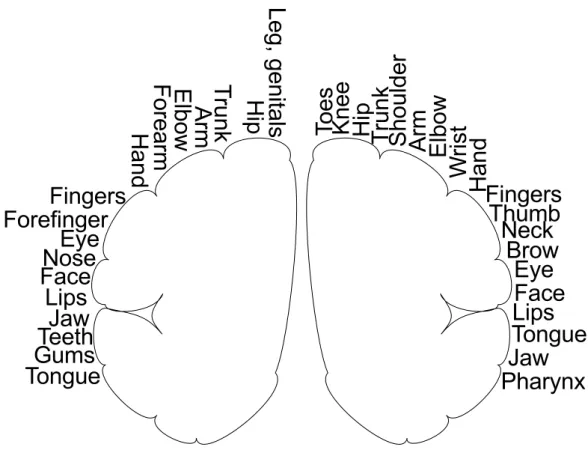
Figure 3.1: Sensory and motor cortex and associated body regions
of brain regions that work for each muscle. Figure 3.1 illustrates which region works for a body region [112].
As shown in Fig. 2.9, the differences in ERD between the different MI tasks are observed. By finding in spatial patterns of ERD, we can associate an observed EEG signal with the MI tasks which a subject performs.
3.2 Discrete Fourier Transform
The features of the MI are observed in frequency domain. Therefore, the signal transformed to the frequency domain can be used as useful features. Discrete Fourier transform (DFT) is the simplest way to obtain the signal in frequency
3.3. COMMON SPATIAL PATTERN 33 domain. Let x∈ RN be a signal observed by an electrode, where N is the number of discrete samples. DFT of x is represented as
[f ]j =
$N k=1
[x]kexp% −2πi( j − 1)(k − 1) N
&
, j =1, . . . , N, (3.1)
where i denotes an imaginary unit defined as i2= −1.
For BMI use, multichannel EEG measurement systems in which many elec- trodes located in different places are used are widely used for improving SNR. Therefore, in case of forming a feature vector with some DFTs, the dimension of the feature vector is large and it causes some problems such as overfitting and an ill-posed problem in classification process.
3.3 Common Spatial Pattern
CSP is a spatial filter. In the definition in the study, the spatial filter works as
y =
$M m=1
wmxm, (3.2)
where, x is a sample observed in the mth channel at a discrete time, wmis a weight coefficient for the signal observed in the mth channel, y is the spatial-filtered signal at the time. The CSP is denoted the vector as w = [w1,w2, . . . ,wM]T.
CSP is found the spatial filter, w ∈ RM, in such a way that the variance of a signal extracted by linear combination of X is minimized in a class [42, 43]. In BCI application, we do not directly use X, but use the filtered signal described as ˆX = H(X) in CSP, where H is a bandpass filter which passes the frequency components related to brain activity of motor imagery. Denote the components of ˆX by ˆX = [ ˆx1, . . . ,xˆN], where ˆxn ∈ RM and n is the time index. The time
average of the observed signal is given by
µ = 1 N
$N n=1
xˆn. (3.3)
Then, the time variance of the extracted signal of ˆX is given by
σ2(X, w) = 1 N
$N n=1
|wT( ˆxn− µ)|2. (3.4)
We assume sets of the learning data, C1and C2, where Cdcontains the signals belonging to class d, d ∈ {1, 2} is a class label, and C1 ∩ C2 = ∅. CSP finds the weight vector that minimizes the intra-class variance in Ccunder the normalization of samples, where c is a class label. More specifically, for c fixed, CSP finds wc by solving the following optimization problem [42, 43];
minw EX∈Cc[σ
2(X, w)],
subject to $
d=1,2
EX∈Cd[σ2(X, w)] = 1,
(3.5)
where EX∈Cd[·] denotes the expectation over Cd. Then, (3.5) can be rewritten as minw w
TΣcw,
subject to wT(Σ1+Σ2)w = 1,
(3.6)
where Σd, d = 1, 2, are defined as
Σd = EX∈Cd
⎡
⎢⎢
⎢⎢
⎢⎣ 1 N
$N n=1
( ˆxn− µ)( ˆxn− µ)T
⎤
⎥⎥
⎥⎥
⎥⎦. (3.7)
The solution of (3.6) is given by the generalized eigenvector corresponding to the smallest generalized eigenvalue of the generalized eigenvalue problem described as
Σcw = λ(Σ1+Σ2)w. (3.8)
3.4. COMMON SPATIO-SPECTRAL PATTERN 35 Although the solution of (3.6) is given by the eigenvector corresponding to the smallest eigenvalue in (3.8), we can use the other eigenvectors for classifica- tion [55]. The M eigenvectors can be obtained by solving (3.8) as ˆw1, . . . ,wˆM,
where ˆwi is the eigenvector corresponding to the ith smallest eigenvalue of (3.8). We assume that the 2r eigenvectors are used for classification of unlabeled data, X. Then we obtain the feature vector, y ∈ R2r, from X defined as
y =[σ2(X, ˆw1), . . . , σ2(X, ˆwr),
σ2(X, ˆwM−r+1), . . . , σ2(X, ˆwM)]T. (3.9)
For classification, y is an input to a classifier such as linear discriminant analysis (LDA) [61].
3.4 Common Spatio-Spectral Pattern
CSSP is a method where a weight vector is obtained by applying the combination of observed signals with time-delayed signals to CSP [44]. Let X ∈ M×N be an observed signal with M channels and N samples. Let X1and X2be the subsignals included in X. The components of X1 and X2 are defined as [X1]m,n = [X]m,n and [X2]m,n = [X]m,n+τ, respectively, where m = 1, . . . , M, n = 1, . . . , N− τ, τ is a sample delay, and [·]i, j denotes the entry in ith row and jth column of a matrix. Then the τ-delay embedded signal is defined as
Xτ=
⎡
⎢⎢
⎢⎢
⎢⎢
⎢⎢
⎢⎣ X1
X2
⎤
⎥⎥
⎥⎥
⎥⎥
⎥⎥
⎥⎦
∈ 2M×(N−τ). (3.10)
CSSP uses Xτto seek the spatial weight vector.
For classification, CSSP can give the feature vector as follows. We obtain 2M
eigenvectors, ˆwi ∈ 2M,i = 1, . . . , 2M, from (3.8) using Xτ. We compose the feature vector, y∈ 2r, in a way similar to (3.9).
In CSSP, the weight vector, ˆwi, can be regarded as a set of FIR filters cor- responding to channels in the following way [44]. Let w0 and wτ be the weight coefficients for the original signal and the delayed signal corresponding to the jth channel in the ith weight vector given by w0 = wˆi[ j] and wτ =wˆi[ j + M], where a[i] denotes the entry of a. Then, the set, {w0,0, . . . , 0
-!!./!!0
τ−1
,wτ}, is regarded as the coefficients of the FIR filter.
3.5 Common Sparse Spectral Spatial Pattern
The CSSSP [45] method obtains a weight vector and an FIR filter by using de- layed signals like CSSP. The main difference between both methods is that CSSSP achieves design of an FIR filter with order more than 2. When CSSSP designs an FIR filter with order T , the optimization problem of CSSSP has the optimization parameters consisting of M spatial weight coefficients and T − 1 coefficients for the FIR filter. Let b1, . . . ,bT be the coefficients of the FIR filter that we want to design. The optimization problem of CSSSP is
max
b2,...,bT
maxw w T
⎛
⎜⎜
⎜⎜
⎜⎜
⎝
T−1
$
τ=0
⎛
⎜⎜
⎜⎜
⎜⎜
⎝
T−τ
$
j=1
bjbj+τ
⎞
⎟⎟
⎟⎟
⎟⎟
⎠Σ
τ c
⎞
⎟⎟
⎟⎟
⎟⎟
⎠w + C T∥b∥1, subject to wT
⎡
⎢⎢
⎢⎢
⎢⎢
⎣
T−1
$
τ=0
⎧⎪
⎪⎨
⎪⎪
⎩
T−τ
$
j=1
bjbj+τ
⎫⎪
⎪⎬
⎪⎪
⎭>Σ
τ 1+Στ2
?
⎤
⎥⎥
⎥⎥
⎥⎥
⎦w = 1,
(3.11)
where b1 is fixed to 1, b is a coefficient vector defined as b = [b1, . . . ,bT]T, Στc is a correlation matrix between the signal, X, and the τ delayed signal, Xτ, defined as
Στc = EX∈Cc
@XXτT +XτXTA, τ > 0, (3.12)