Progressive 3D Animated Models for Mobile & Web Uses
Bing-Yu Chen* Sheng-Yao Cho
†Henry Johan
‡Tomoyuki Nishita
‡*
†National Taiwan University
‡The University of Tokyo
*[email protected]
†[email protected]
‡{henry, nis}@is.s.u-tokyo.ac.jp
Abstract
To date, more high resolution 3D animated models are required to present important details and fine structures, however, sometimes such high resolution models are un- necessary and undesired, especially on web and mobile phone environments. Though there are many well-known algorithms dealing well on simplifying 3D models, most of them are limited to static ones. Applying these mesh sim- plification methods to 3D animated models, a good sim- plified model in a specified pose can be obtained. How- ever, some features of the original animated model, which can be shown in other poses, may be destroyed. In this paper, we propose an automatic method to simplify a 3D animated model which takes the features shown in every poses into account and preserves the geometry details of them. Therefore, a progressive 3D animated model can be generated for mobile or web uses.
Keywords: Progressive Animated Models, Animated Model Simplification, Level-of-Details.
1. Introduction
Progressive Meshes (PM) [9] is a famous method for constructing a sequence of 3D models with continuous level-of-detail (LOD) based on recursive edge collapse operations. It can be used widely not only for displaying a 3D model with continuous LOD, but also for transmitting the 3D model over the Internet. The 3D model here only means a static 3D model without motion data. However, the 3D model with motion data, or so-called 3D animated model, is more widely used in many fields, like on-line games, animations, etc. Therefore, how to provide a method similar with PM but for the 3D animated model is necessary. In this paper, we present a novel scheme to construct a sequence of 3D animated models with LOD based on PM and the mesh simplification method pre- sented by Garland and Heckbert [6], which is known as the Quadric Error Metric (QEM) method. The generated progressive 3D animated model can be used for web presentation or showing on hand-held devices.
In general, most of the mesh simplification methods are based on the error approximation of a 3D model in a sin- gle pose, since most of the 3D models are static. These methods can result good simplified models in a neutral pose. However, when applying these methods to an ani-
Figure 1, it may destroy some features of the cat model in some particular poses. As an example shown in Figures 2 (a) and (b), which are the first and third frames of the sim- plified animated model of Figure 1. The simplified ani- mated model is obtained by using the QEM method which only references the first pose of the animated model and applies the simplification process to all of the poses. Hence, the features which can be detected at the first frame can be reserved, but the features which are hidden at the first frame are ignored.
(a) (b) (c) (d) (e) Figure 1. Five poses of an original 3D animated model, which is composed of 31 3D models and every model is deformed from the same cat model. (a) ~ (e) shows the poses at the first, third, sixth, eighth, and tenth frame, re- spectively.
(a) (b)
(c) (d) Figure 2. (a) (b) The simplified models of the first and
third frames when simplifying the animated model by only considering the first frame. (c) (d) The simplified models of the first and third frames when using our method. Ob- viously, the shape of the cat’s tail shown in (b) and (d) are different. The carved shape of the cat’s tail is preserved in our method.
The simplified models shown in Figures 2 (c) and (d)
Figures 2 (b) and (d), although the two models have the same number of triangles, the curved shape of the tail part is preserved in Figure 2 (d) as Figure 1 (b), but that is not preserved in Figure 2 (b).
The major contribution of our method is that we pro- pose a mesh simplification method for 3D animated model while preserving the features of the model, even the fea- tures are only shown in a few frame. This paper has been presented in NICOGRAPH International 2005. [4]
2. Related Work
PM provided by Hoppe [9]is a famous method for 3D mesh simplification and is based on the edge collapse or edge contraction operation. Although this method could result in an almost optimized simplified model, it is well known to be time-consuming. A derived method, QEM[6], has been provided to make the calculation faster. Instead of using edge collapse or edge contraction operation for edge or vertex removal, it uses vertex-pair collapse opera- tion which is also similar with edge collapse or edge con- traction operation. The heuristic function used by QEM is geometry-based, since it calculates the geometric distance between the newly generated vertex and the faces which are deformed before generating it. Both of them are good methods for simplifying static 3D models for continuous LOD.
For simplifying 3D animated models, Alexa and Müller [1] proposed an approach to represent time-varying ge- ometry by principal components. Through their method, a matrix composed of consistent meshes of original key-frames is build at first. The vertices of each frame of this matrix are then decomposed to the bases and weights after a Singular Value Decomposition (SVD) operation. By adapting different number of the basis, the LOD can be achieved. It also supports progressive animation compres- sion with spatial, as well as temporal. However, the com- putational time for SVD decomposition is expensive and the view-dependent property cannot be fulfilled with this approach. Kircher and Garland also provide a method for this problem [11].
Houle and Poulin presented a very similar algorithm as ours on skeletal meshes [10]. They combined the PM con- cept and skeletal models to produce animation with con- tinuous LOD. Their contribution is major for game indus- try, especially on-line games; however, it is limited to the models with skeleton, e.g. human or animals. Furthermore, they simplify the articulated mesh by taking only one sin- gle static model into account without considering the all poses contained in the animation sequences, so they had to adjust the model to a special pose by hand for better sim- plification effect.
Shamir and Pascucci proposed a scheme for creating LOD models for time-dependent meshes [12]. It supports
both temporal and spatial LOD. They divided temporal variation into factors with low and high frequencies. In their definition, low-frequency factor stands for global affine transformation while high-frequency factor stands for local vertex deformations. They had different and good LOD effects by applying different updates (e.g. spatial and temporal); however, the size of the encoded data is much larger than the original mesh.
Based on "Geometry Images" [7], Briceno et al. pro- posed "Geometry Videos" [3] as a new representation for 3D animation. For each key-frame model, it uses global cut algorithm and parameterization method to create con- sistent geometry images. It inherits many advantages from Geometry Images and provides meshes in each frame with regular connectivity, LOD, and allows for applying nu- merous processing and compression methods targeted at videos to animated models. Though it has several advan- tages over previous techniques; however, for models with high-genus, it will cause high distortion due to the defeats of Geometry Images.
3. Animated Model Simplification
3.1 3D Animated Model
In this paper, we describe an animation comprised of a sequence of 3D animated models which are denoted as
ˆ ˆ0
i i
M =M + ∆M for the i-th key-frame, where Mˆ0 is a generic triangle mesh; each animated model is deformed from it, and it can also be the model at the first key-frame, i.e., Mˆ1=Mˆ0. ∆Mi means the geometric difference of the i-th key-frame between Mˆi and Mˆ0, which is gen- erated by the object’s skeleton or other deformation meth- ods like other animation generating methods. Then, the state of the object can be calculated by interpolating two in-between models on two consecutive key-frames. There- fore, if the number of polygons of the object is large, to generate the model sequence is a time-consuming task. 3.2 Simplification Scheme
To decrease the number of polygons of the object is a good idea to solve the problem. However, if we simplified the 3D animated models by simplifying each pose sepa- rately using traditional mesh simplification method, the interpolation of two in-between models may be an artifact. To make the simplified animated models consistent as the original model sequence, we only simplify the initial mesh
0 0
ˆ n
M =M into a coarser mesh M00 by applying a se- quence of n successive edge collapse operations. Since edge collapse operations are invertible, Mˆ0 can therefore
be denoted as its simplified mesh M00 with a sequence of n vsplit records as described in [9], where vsplit is a ver- tex split operation which is the inverse operation of edge collapse. Hence, Mˆ0 =M0n can be denoted as
0
0 0 0 1
ˆ n n
j j
M =M =M +
∑
= vsplit .Then, the pose of the animated model at the i -th key-frame can be defined as
0
0 0 1
0 1
ˆ ˆ n
i i j j i
n n
i j j i
M M M M vsplit M
M vsplit M
=
=
= + ∆ = + + ∆
= + =
∑ ∑
.Therefore, by applying some vsplit records to Mi0, we can get multiresolution animated models for each key-frame.
Figure 3. The features which are only appeared in some certain frames can be detected by considering their QEM values.
3.3 The QEM Function
To simplify the initial mesh Mˆ0, we use the algorithm modified from the QEM method. The original QEM method simplifies the mesh by considering the quadric error metrics Q( )v of each vertex v of the mesh. If
( )v
Q is large, that means the vertex v is located at a bumpy surface and it might be a feature and will be re- moved later. Otherwise, it will be removed earlier. Since the initial mesh Mˆ0 is deformed to be other poses to per- form the animated model, to simplify it, it is necessary to take other poses of the animated model into account at the same time.
In Figure 3, we show the variance of two QEM values of two vertex-pairs along the time. During the animation playing, the QEM values of some vertices might be
changed. That means a vertex will be the feature at certain frame, but it can be removed at other frames since it is not the feature in these frames. If we do not consider this situation and just remove it since it is not the feature in most frames, the feature will be disappeared like the curved shape of the tail part shown in Figure 2 (b).
Hence, we modified the quadric error metrics Q( )v of each vertex v of the initial mesh Mˆ0 to be
( )v =max i( )v
Q Q , where Q( )v is the quadric error met- rics of the corresponding vertex v of the animated mod- els Mˆi for the i-th key-frame. The value of Q( )v is used to select a proper vertex v with the minimum
( )v
Q to remove. Hence, we use the maximum Q( )v , among the key-frames to guarantee the removed vertex is the proper one for all of the models which composed the animated model. To drive M0j by adding ∆Mi, i.e.,
0
j j
i i
M =M + ∆M , a deformed model at the i -th key-frame and j-th level can be achieved. The geometric difference ∆Mi is generated by the model’s skeleton or some deformation methods, so when applying ∆Mi to
0
Mj, if some parts or vertices of the model has been sim- plified, this geometric difference will be ignored. That means if a part of the model has been removed, the motion of this part should also be ignored.
The reasons that we use this QEM function are based on the following two heuristics: (1) The decimation cost of the original features of the initial model are certainly high within all frames. (2) Features caused by the deformation will introduce the peaks of the QEM value as shown in Figure 3. From the first heuristic, we can still preserve the original features of the animated model because those fea- tures are motion independent, and the second one takes the features caused by some specific motions into account whether those motions are frequent or not. If the motion is frequent in this animation, it will introduce many peaks of QEM value in the chart.
4. Result
Figure 4 shows the simplification result of an angry cat animation which is composed by 31 cat models with dif- ferent poses. Obviously, even the number of triangles is much decreased; the features of the animation can still be recognized, such as the curved shape of the tail part and the variance of the cat’s back.
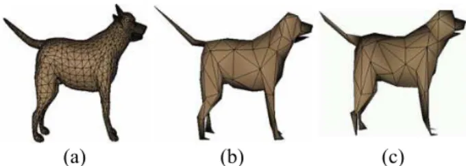
The lower row of Figure 5 shows a dog walking animation which is generated by 20 deformed dog models. Since the entire animated dog models are generated by deforming the same initial dog model, these models are vertex-wise correspondence. Simplifying the initial dog model while
considering the quadric error metrics of the other poses, the multiresolution dog walking animation can be obtained as the upper and middle rows of Figure 5. Applying the deformation data to the simplified dog models, multireso- lution dog walking animations can be obtained. To sim- plify the dog models, it costs about 3.76sec. on a desktop
PC with an Intel Pentium 4 2.6GHz CPU. The perform- ance of simplification depends on the number of vertices of the initial model and the key-frame number of the ani- mation. To display our progressive 3D animated model, we provide the viewers on several platforms including web environments and mobile phones.
Figure 4. An angry cat animation. The lower row shows five poses of the original animated model. The model consists of 5,400 triangles. The middle and upper rows show the corresponding simplified results, which consist of 1,000 and 100 triangles, respectively.
Figure 5. A walking dog animation. The lower row shows five poses of the original animated model. The model consists of 8,136 triangles. The middle and upper rows show the corresponding simplified results, which consist of 1,000 and 150 triangles, respectively.
To compare our method with other simplification schemes, we use two kinds of quadric error metrics:
( )v = 0( )v
Q Q and Q( )v =
∑
mi=−01Qi( ) /v m, where m is the number of frames and Q1( )v =Q0( )v . We call the two kinds of QEM functions as single pose approach and average poses approach. The result of us- ing single pose approach is like the result of [10], since both of single pose approach and [10] only consider the features appeared in one certain frame. Hence, as shown inFigure 2 (b), the curved shape of the tail part of the cat model will be simplified since that part was not a feature at the initial model. Someone may want to use the average QEM value for simplification as average poses approach. As shown in Figure 6 (c), compare to Figure 6 (b), the back feet part of Figure 6 (c) becomes strange, since av- erage poses approach makes the importance of that part decreased. This is because that part is not always the fea- ture.
To measure the statistic differences of these simplifica- 150 triangles
1000 triangles
8135 triangles 100 triangles
1,000 triangles
5,400 triangles
tion schemes, we use Metro [5] as a measuring tool to compare the simplified models to the original ones. It is designed to compensate for a deficiency in many simplifi- cation methods proposed in literature. It allows one to compare the difference between a pair of surfaces (e.g. a triangulated mesh and its simplified representation) by adopting a surface sampling approach. It has been de- signed as a highly general tool, and it does no assumption on the particular approach used to build the simplified representation. It can also return both numerical results (meshes areas and volumes, maximum and mean error, etc.) and visual results, by coloring the input surface ac-
cording to the approximation error.
(a) (b) (c) Figure 6. (a) The original dog model which is the first pose of a dog animation sequence. (b) The simplified dog model generated by our method. (c) The simplified dog model generated by using average poses approach.
(a) (b) (c) Figure 7. RMS distance between the simplified animated model and the original one for (a) our method, (b) simplification
due to the first frame as single pose approach, and (c) simplification using average poses approach.
(a) (b) Figure 8. Progressive animated model viewer on (a) a mo-
bile phone and (b) a Java-enabled browser.
For each simplified model (in different level and dif- ferent frame), we measure the root mean square (RMS) distance from its surface to the corresponding model (in the same frame but full resolution). Then Matlab1 is used to make charts for observation: x-axis stands for the level (from 10 to 1) of the simplified model, where level-10 is the full resolution and level-1 contains 10% faces of the original model; y-axis stands for the frame number, and z-axis stands for the measured error approximations.
1 http://www.mathworks.com/
Figure 7 shows the RMS distance approximation of all simplified models generated by three different simplifica- tion approaches. RMS distance is a better measurement or metric than mean distance, because it is two-norm dis- tances and it considers the space-relationship of distances between sampled points on original model and simplified model. From Figure 7, we find out that the RMS distance between the original model and the simplified model are smaller if we use our method or average poses approach. Another observation is that the surface of the chart created by our method is much smoother than those by other sim- plification approaches. That means some features are sim- plified in other two approaches, so at some certain frames, the differences between the simplified model and the original one become large and it makes the chart becomes bumpy.
Since the target of our method is to provide a progres- sive animated model for web and mobile uses, we there- fore provide two kinds of viewers as shown in Figure 8. One is developed for mobile phones and the other is for Java-enabled browsers.
5. Conclusions and Future Work
In this paper, a fully automatic simplification scheme, which preserves the deformation features of objects, for animated models is proposed. 3D animated models, either key-framing or skeletal models, can be inputs of our sys-
tem, and a progressive animated model is generated. The scheme we proposed takes every pose of the animated model into account, and determines a better decimation sequence to simplify it. We can find out that our method really produce better simplified models than other schemes from the visualized results. Moreover, we can conclude that our method can generate a smooth animated model from the statistic results, though the evaluation of error approximation of our method is slightly higher than the average scheme.
Currently our simplification method does not consider the attributes of the vertices, like colors, textures, and even the binding weights of the skeletal models. Though the animated model is scalable, the storage space is huge. We would like to propose a well-organized data structure to store those data in the near future. The TDAG (Temporal Directed Acyclic Graph) structure used by Shamir and Pascucci in [10] is a good reference for us to start.
Acknowledgements
This work was partially supported by the National Sci- ence Council of Taiwan under the numbers: 92-2218-E- 002-056, 93-2213-E-002-084, and 94-2213-E-002-097. The third author, Henry Johan, is supported by the Japan Society for the Promotion of Science (JSPS) Postdoctoral Fellowship for Foreign Researchers.
References
[1] M. Alexa and W. Müller. Representing animations by principal components. Computer Graphics Forum (Eurographics 2000 Conference Proceedings), 19(3):411–418, 2000.
[2] C. L. Bajaj, V. Pascucci, and G. Zhuang. Progressive compressive and transmission of arbitrary triangular meshes. In IEEE Visualization 1999 Conference Pro- ceedings, pages 307–316, 1999.
[3] H. M. Briceno, P. V. Sander, L. McMillan, S. Gortler, and H. Hoppe. Geometry videos: a new representation for 3D animations. In Proceedings of ACM Sympo- sium on Computer Animation 2003, pages 136–146, 2003.
[4] B.-Y. Chen, S.-Y. Cho, H. Johan, and T. Nishita. Pro- gressive 3D animated models for mobile & web uses. In NICOGRAPH International 2005 Conference Pro- ceedings, pages 135-140, 2005.
[5] P. Cignoni, C. Rocchini and R. Scopigno. Metro: measuring error on simplified surfaces. Computer Graphics Forum, 17(2):167–174, 1998.
[6] M. Garland and P. S. Heckbert. Surface simplification using quadric error metrics. In ACM SIGGRAPH 1997 Conference Proceedings, pages 209–216, 1997. [7] X. Gu, S. J. Gortler, and H. Hoppe. Geometry images.
ACM Transactions on Graphics (SIGGRAPH 2002 Conference Proceedings), 21(3):355–361, 2002. [8] A. Gueziec, G. Taubin, B. Horn, and F. Lazarus. A
framework for streaming geometry in VRML. IEEE Computer Graphics and Applications, 19(2):68–78, 1999.
[9] H. Hoppe. Progressive meshes. In ACM SIGGRAPH 1996 Conference Proceedings, pages 99–108, 1996. [10] J. Houle and P. Poulin. Simplification and real-time
smooth transitions of articulated meshes. In Graphics Interface 2001 Conference Proceedings, pages 55–60, 2001.
[11] S. Kircher and M. Garland. Progressive Multiresolu- tion Meshes for Deforming Surfaces. In Proceedings of ACM Symposium on Computer Animation 2005, 2005.
[12] A. Shamir and V. Pascucci. Temporal and spatial level of details for dynamic meshes. In Proceedings of ACM Symposium on Virtual Reality Software and Technology 2001, pages 77–84, 2001.
[13] M. Soucy and D. Laurendeau. Multiresolution surface modeling based on hierarchical triangulation. Com- puter Vision and Image Understanding, 63(1):1–14, 1996.
[14] J. Rossignac and P. Borrel. Multi-resolution 3D ap- proximations for rendering complex scenes. In Pro- ceedings of Geometric Modeling in Computer Graph- ics, pages 455–465, 1993.