本文 Thesis 総合研究大学院大学学術情報リポジトリ A1669本文

The Graduate University for Advanced Studies

School of High Energy Accelerator Science

Department of Particle and Nuclear Physics

Higgs interactions

in physics

beyond the standard model

Yohei Kikuta

A dissertation submitted in partial fulfillment

of the requirement for the degree of

Doctor of Science in Physics

Abstract

In this thesis we study the Higgs interactions in physics beyond the Standard Model. After the discovery of the Higgs boson at the LHC, it is the time to study the Higgs interactions from various aspects. The precise measurement of the Higgs boson properties provides tests of the Standard Model, and perhaps the first signal of new physics beyond the Standard Model can be indirectly found in Higgs physics. In this thesis we concentrate on the following two issues: the scattering amplitudes of the longitudinal gauge bosons and the Higgs boson, and the couplings of the Higgs boson to other particles. The first one is related to the perturbative unitarity of a theory with spontaneously broken symmetries and expected to be important information for the scalar sector, especially the origin of the electroweak symmetry breaking. The second one reflects the structure of the Higgs interactions and gives a clue for the mass generation of the particles. Various new physics models show the deviations of these properties from the Standard Model prediction, which may be investigated at the future collider experiments. We examine the unitarity violation caused by the dimension-six derivative interactions of the Higgs doublets, which indicates the new physics scale associated with an extended Higgs sector. We compute the strongest unitarity bound for several models and find it gives rather low cut-off scale compared with that of the naive dimensional analysis. We also examine the possible deviations of the Higgs couplings in agreement with the experimental constraints, focusing on the three models: the minimal composite Higgs models, the Randall-Sundrum model, and the extra singlet Higgs model. It is found that the correlation of Higgs couplings is quite powerful to discriminate models at the future collider experiments.

This thesis is composed of five chapters. In chapter 1 we give an overview of the current status of phenomenological particle physics, especially about Higgs physics. While all the particles of the Standard Model are observed, we know the phenomena the Standard Model seems not to cover; hence there are many proposals for new physics beyond the Standard Model. In chapter 2 we provide a brief overview of Higgs physics in the Standard Model. The Higgs sector is introduced to account for the low energy breaking of the SU (2)_L×U(1)Y electroweak gauge symmetry to the U (1)_EM, and all of the interactions including the Higgs boson is determined by its mass value. In chapter 3 we analyze the perturbative unitarity bound given by the dimension-six derivative interactions consisting of the Higgs doublets. The bound is obtained by diagonalizing the scattering amplitude matrix of two-body to two-body scattering processes which include the longitudinal gauge bosons and the Higgs boson. We formulate it in terms of the parameters of the Lagrangian. In chapter 4 we present the deviations of the Higgs couplings in some models, compared with the Standard Model prediction, mainly focusing on the minimal composite Higgs model. In order to classify the features of the models we consider, we elucidate the correlation of the coupling deviations. The future experiments are able to distinguish the models well by using both the tree level and loop induced Higgs couplings. In the concluding remarks we summarize our results and give an outlook for the future prospects of Higgs physics.

Contents

1 Introduction 1

2 Higgs physics in the Standard Model 3

2.1 Lagrangian including the Higgs field 3

2.1.1 Higgs potential part 4

2.1.2 Higgs kinetic part 4

2.1.3 Yukawa interaction part 5

2.2 Higgs interactions with other particles 7

2.2.1 Tree level interactions 8

2.2.2 One-loop level interactions 9

2.2.3 Experimental sensitivity to the Higgs couplings 11

2.3 Theoretical aspects of Higgs physics 14

2.3.1 Perturbative unitarity 14

2.3.2 Custodial symmetry 17

2.3.3 Equivalence theorem 18

2.3.4 Higgs low energy theorem 20

2.3.5 Fine tuning problem 22

3 Perturbative unitarity of Higgs derivative interactions 23 3.1 Unitarity of derivative interactions on one Higgs doublet models 24 3.1.1 Formulae and general properties of the unitarity bound 25

3.1.2 The minimal composite Higgs model 28

3.1.3 The littlest Higgs model with T-parity 28

3.2 Unitarity of derivative interactions on two Higgs doublet models 29 3.2.1 Formulae and general properties of the unitarity bound 29

3.2.2 The bestest little Higgs model 30

3.2.3 The UV friendly little Higgs model 32

3.2.4 Inert doublet models with odd scalars 34

3.3 Conclusions 37

4 Higgs couplings beyond the Standard Model 38

4.1 The minimal composite Higgs model 38

4.1.1 The Lagrangian 39

4.1.2 Experimental constraints 45

4.1.3 Decay widths and couplings: numerical result 50

4.2 Other models 56

4.2.1 Randall-Sundrum model 57

4.2.2 Extra singlet Higgs model 62

4.3 Model discrimination using the correlation of Higgs couplings 63

4.4 Conclusions 67

5 Concluding remarks 68

A Loop functions and special functions 70

B Unitarity matrices and other bounds 73

B.1 Neutral two-body states 73

B.2 Singly charged two-body states 75

B.3 Doubly charged two-body states 76

C Custodial symmetry of derivative interactions 77

1 Introduction

The Higgs boson which is predicted by the Standard Model (SM) has been discovered by the ATLAS and CMS experiments at the LHC in 2012 [1]. This observation means that the spontaneous symmetry breaking (SSB) by the condensation of the scalar field, Brout-Englert-Higgs mechanism [2], occurs in the real world. The vacuum expectation value (VEV) of the Higgs field gives the masses of W/Z bosons, quarks, charged leptons and the Higgs boson itself; the strength of the interaction with the Higgs field is completely determined by the mass of the interacting particle. Although we have observed only the gauge interactions as a fundamental interaction so far, the discovery of the Higgs boson and the SSB strongly implies the existence of the yukawa interaction (at least the top yukawa interaction) and the Higgs self interaction. Now the experiments shed light on the Higgs sector, and the SM is being confirmed; the establishment of the SM is one of the greatest achievement of human intellect.

While the SM can explain extraordinarily well physical phenomena observed at the microscopic scale, there exists a number of the experimental and the theoretical problems which the SM cannot answer: neutrino masses and oscillations, dark matter, baryon asym- metry of the universe, inflation, fine tuning problems, impossibility of the unification of the gauge couplings, and so forth. We have to introduce a new element into the theory to solve these problems: symmetries, particles, mechanisms. Such extensions of the SM probably leave traces of physics beyond the SM; we try to find them by means of direct and indirect measurements. A direct measurement is the method to search new phenomena which are undoubtedly signals of new physics. An indirect measurement is the method to investigate the deviations from the SM prediction, which can be more powerful than a direct one in some cases. These two ways are complementary, and they allow us to investigate various features and properties of the model we consider.

With regard to the Higgs sector, one of the important problems is the mystery of why the electroweak (EW) symmetry is spontaneously broken. This mystery is deeply connected with the Higgs fine tuning problem which requires unnatural adjustment of the dimension- full Higgs mass parameter to produce the correct EW scale. Since the EW symmetry is

broken by hand via the negative mass-squared term in the case of the SM, the model does not tell us the origin of the SSB and cannot avoid the unacceptable fine tuning of the Higgs mass parameter. It would be undesirable for the fundamental theory of nature, and we expect that some mechanism or dynamics naturally explains the EW symmetry breaking and stabilizes the EW scale. In order to provide the natural description of the Higgs sector at the EW scale, we have to construct a TeV-scale theory that will replace the SM.

Many models describing the physics beyond the SM have been proposed: supersym- meric (SUSY) models, composite Higgs models and models with extra dimensions, etc. The Higgs sector of these models is extended as it is naturally responsible for the EW symmetry breaking with a certain dynamics or mechanism. Such an extension of the Higgs sector causes the modification of Higgs physics from that of the SM. The modification can affect various observables at the collider experiments; maybe its effect could be firstly observed as deviations from the SM prediction at the energy scale which is lower than a typical new physics scale (such as the dynamical scale or the masses of new resonances). From the perspective of the effective theory, we can examine these deviations in terms of higher dimensional operators including the Higgs field. Higgs physics is therefore important not only for the establishment of the SM Higgs sector but also for the indirect search of the new physics. After the discovery of the Higgs boson, it is becoming more important and interesting to investigate the phenomena beyond the SM by focusing on Higgs physics. In this thesis we concentrate on Higgs physics as a window to new physics and especially study the following two subjects.

One of the topics we study is the perturbative unitarity of the scattering amplitudes of the longitudinal gauge bosons and Higgs bosons [3]. Since the massive gauge boson has the longitudinal polarization state whose wave function is proportional to the four momentum in the high energy limit, the massive gauge boson scattering amplitudes grow as the center of mass energy increases. In the case of the SM the contribution from the Higgs boson cancels the positive power dependence of energy on the amplitudes, and the amplitudes are expressed as a function of the Higgs mass; hence the unitarity of the theory is ensured [4]. This is the striking feature of the renormalizable spontaneously broken gauge theory. However, if there is a deviation of the coupling between the gauge bosons and the Higgs boson, such a cancellation would be lost. The amplitudes therefore keep growing until the energy scale where the perturbative unitarity breaks down, which suggests that some new physics has to appear at this energy scale and recover the unitarity of the theory. Typically, the dimension-six derivative interactions of the Higgs field give rise to the unitarity violation in the high energy region [5]. It is meaningful to estimate the energy scale of the unitarity violation within the effective theory in which heavy particles are integrated out and only the SM particles including the Higgs bosons are treated as a dynamical degrees of freedom (DOF). According to the Ref [6], the general form of the dimension-six derivative interactions including any number of the Higgs doublets is constructed. With this consequence we examine the condition of the tree level unitarity violation in terms of the coefficients of the dimension-six Higgs derivative operators for the one Higgs doublet and two Higgs doublets cases. By way of example, we show the typical unitarity violation scales in various composite Higgs models; however our result can be

applied to any theory where the dimension-six Higgs derivative interactions are generated. The other topic is the couplings of the Higgs boson to other particles. For the SM the strength of the couplings is expressed in terms of the particle mass and the VEV of the Higgs field, and we already know all of the mass parameters in the theory. Hence the deviation of the couplings from those of the SM is undoubtedly evidence of new physics. In most cases new physics models predict the modified Higgs couplings at tree or loop level. These modified couplings are good observables for the search of new physics. At this stage, the Higgs couplings begin to be observed at the LHC [7]. At the future collider experiments we can measure the various couplings with high accuracy, ≤ O(1)%, which is a powerful tool for probing new physics; the more precise the experiment, the higher scale physics we can probe. In addition, the correlations of the modified Higgs couplings are useful to discriminate new physics models because they tend to show different features for each model. In this work we especially study the partial decay widths and the couplings of the Higgs boson in the minimal composite Higgs model (MCHM) [8] in detail. It is notable that we compute all of the loop induced effective couplings, hgg, hγγ and hZγ, including exact mass dependences of the heavy resonances and show their correlations. Then the result is compared with those of other models, the Randall-Sundrum (RS) model [9] and the extra singlet Higgs model. Using the correlations of the deviations of the Higgs couplings, we clarify how we can discriminate each model in the future experiments.

2 Higgs physics in the Standard Model

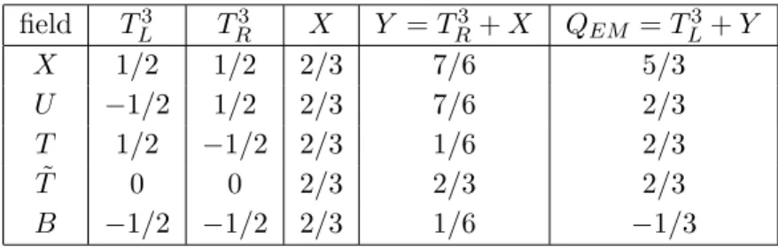
In this chapter we briefly review the Higgs physics in the SM. The Higgs field is introduced as (1, 2, +1/2)¹ under SU (3)_{C× SU(2)L× U(1)Y}, and its VEV breaks SU (2)_{L× U(1)Y} down to U (1)_EM [10]. The Higgs interactions are completely determined by the masses of the interacting particles.

2.1 Lagrangian including the Higgs field

The Lagrangian including the Higgs field is divided into three parts:

L ⊃ LV ⁺LHkin⁺Lyukawa^{, (2.1)}

where _LV,_LHkin and _Lyukawa are Higgs potential part, Higgs kinetic part and yukawa interaction part. The Higgs field can be parametrized using four real DOFs as

H(x) = _√¹ 2

(h₁(x) + ih₂(x) h₃(x) + ih₄(x)

)

. (2.2)

1We define the hypercharge as Y = Q − TL³.

2.1.1 Higgs potential part

Higgs potential is described by two parameters: LV ^{= µ2}|H|²− λ|H|⁴⁼−λ

(

|H|²− ^µ

2

2λ )2

+^µ

4

4λ^{. (2.3)}

The VEV reads _{⟨|H|⟩ ≡ v/}^√2 =√µ²/2λ. This non-trivial VEV is essential for the EW symmetry breaking; the trigger is the sign of the mass parameter µ² which is chosen by hand and the reason cannot be explained in the SM. After expanding around the VEV and using an SU (2)_W rotation, the Higgs doublet can be expressed as

H(x) = U (x)_√¹ 2

( 0

v + h(x) )

, (2.4)

where U (x) is a gauge transformation of SU (2)_W. We can always rotate away this U (x) by transforming H(x)_{→ U}⁻¹(x)H(x), which means that only one DOF remains physical after the SSB. The other three DOFs are called Nambu Goldstone (NG) bosons and ”eaten” by gauge bosons as we will see.

In the basis where U (x) is rotated away, so-called unitary gauge, we are able to rewrite LV^:

LV ⁼−λv^2h2− λvh³−^λ 4^h

4

=₋¹ 2^m

2h^h2− ^m

2h

2v ^h

3₋ ^m2h

8v^2h

4_{, (2.5)}

where m_h is the Higgs mass. Now we have measured the value of the mass of the Higgs boson:

m_h= 125.9± 0.4 [GeV]. ^(2.6)

Note that we drop the vacuum energy term in the Eq. (2.5); we need not care about it as long as neglecting the gravity.

2.1.2 Higgs kinetic part The Higgs kinetic term reads

LHkin ^{= (D}µ^{H)†DµH, D}µ^{= ∂}µ− igWµ^a

σ^a 2 ^{− i}

g^′

2^{BµI2×2, (2.7)} where σ^a (a=1,2,3) is the Pauli matrices. We then move to the electromagnetic eigenbasis since U (1)_EM gauge symmetry still remains after the EW symmetry breaking:

W_µ^± = _√¹ 2^(W

µ1∓ iWµ^{2), (2.8)}

Z_µ= ¹

√g²+ g^′2(gW

µ3− g^′Bµ^{) = cos θ}W^Wµ³− sin θW^Bµ^{, (2.9)}

A_µ= ¹

√g²+ g^′2(g

′_W³

µ^{+ gB}µ^{) = sin θ}W^Wµ^{3+ cos θ}W^Bµ^{, (2.10)}

where θ_W is the Weinberg angle. In this basis we get

LHkin ⁼

1 2^∂µh∂

µ_{h +}^(gv

2 )2

W_µ⁺W^−µ (

1 +^h v

)2

+

( √g²+ g^′2v 2

)2

ZµZ^µ 2

( 1 +^h

v )2

= ¹ 2^∂µh∂

µ_{h + m}2

W^Wµ^+W−µ

( 1 +^h

v )2

+ m²_Z^ZµZ

µ

2 (

1 +^h v

)2

. (2.11)

2.1.3 Yukawa interaction part

The yukawa interaction Lagrangian is the following: Lyukawa⁼−

3

∑

I,J

L¯^g_Iy_IJ^l,ge^g_JH₋

3

∑

I,J

Q¯^g_Iy_IJ^d,gd^g_JH₋

3

∑

I,J

Q¯^g_Iy_IJ^u,gu^g_JH + (h.c.),^˜ (2.12)

where superscript g means the gauge eigenbasis, and l, d and u stand for lepton, down quark and up quark respectively. We also define

H = iσ˜ ²H^∗, (2.13)

L_I = (ν_e

e )

L

, (ν_µ

µ )

L

, (ν_τ

τ )

L

, (2.14)

Q_I = (u

d )

L

, (c

s )

L

, (t

b )

L

, (2.15)

e_I = e_R, µ_R, τ_R, (2.16)

d_I = d_R, s_R, b_R, (2.17)

uI = uR, cR, tR. (2.18)

Here L(R) denotes the left (right) handedness. It is notable that in the Eq. (2.12) only the left handed neutrino is introduced; hence the neutrinos are massless in the SM. Let us count the DOFs of the yukawa couplings. If y = 0, the Lagrangian is invariant under the chiral transformations:

L^g_{I → FLIJ}L^g_J, e^g_{I → FeIJ}e^g_J, (2.19) Q^g_{I → FQIJ}Q^g_J, d^g_{I → FdIJ}d^g_J, u^g_{I → FuIJ}u^g_J, (2.20) where F is 3× 3 unitary matrix acting on flavor space. The yukawa couplings break these symmetries explicitly. Let us treat the yukawa couplings as spur ions transforming as follows:

y^lg_{IJ → FLII}′y_I^lg_′J′F_eJ^† _′J, (2.21) y^dg_{IJ → FQII}′y^dg_I′J′F_dJ^† _′J, (2.22) y^ug_{IJ → FQII}′y^ug_I′J′F_uJ^† _′J. (2.23)

The Lagrangian is still invariant under these transformations. Note that if we choose F_Q= F_u = F_d = e^iB and F_L= W diag(e^iα, e^iβ, e^iγ), F_e = W diag(e^iα, e^iβ, e^iγ) where W^†y^lgW = diag(y₁, y₂, y₃), the yukawa Lagrangian remains invariant. These are corresponding to the baryon number conservation and the lepton number conservation for each generation. Similarly to the NG boson case, we could write the physical DOF of the yukawa couplings as

N_{y phys}= N_{y− NG}+ N_G′, (2.24)

where a chiral symmetry G is broken explicitly by the yukawa sector to a group G^′. For the lepton sector, G = U (3)_{L⊗ U(3)e} and G^′= U (1)³. Then we get

moduli : Ny phys= 3²_{− 2}^{3(3− 1)}

2 ^{= 6, (2.25)}

phases : N_{y phys}= 3²_{− 2}^{3(3 + 1)}

2 ^{+ 3 = 0. (2.26)}

The half of moduli is related to masses, and the others are corresponding to physical yukawa couplings. For the quark sector, G = U (3)_{Q⊗ U(3)u⊗ U(3)d} and G^′= U (1)_B, leading to

moduli : N_{y phys}= 2_{× 3}²_{− 3}^{3(3− 1)}

2 ^{= 9, (2.27)}

phases : N_{y phys}= 2_{× 3}²_{− 3}^{3(3 + 1)}

2 ^{+ 1 = 1. (2.28)}

The moduli are divided into three masses, three mixing angles and three yukawa couplings. We have one phase DOF in the quark sector which is the unique source of the CP-violation in the SM.

In order to get the mass eigenstates we perform the singular value decomposition (SVD) by defining the following unitary matrices:

3

∑

I,J=1

(U_iI^l )^†y^l,g_IJV_Jj^l = δijy_i^l, (2.29)

3

∑

I,J=1

(U_iI^d)^†y_IJ^d,gV_Jj^d = δ_ijy_i^d, (2.30)

3

∑

I,J=1

(U_iI^u)^†y_IJ^u,gV_Jj^u = δ_ijy_i^u. (2.31) The relations between the gauge eigenstates and the mass eigenstates are

e^g_I = V_Ii^lei, (2.32)

d^g_I = V_Ii^dd_i, (2.33)

u^g_I = V_Ii^uu_i, (2.34)

L¯^g_I = ¯L_i(U_iI^l )^†, (2.35)

Q¯^g_I = (¯u_i(U_iI^u)^†, ¯d_i(U_iI^d)^†)_L= (¯u_i, ¯d_j(V_ji^CKM)^†)_L (U_iI^u)^†

= (¯ui, ¯d^′i)_L (U_iI^u)^†= ¯Q_I(U_iI^u)^†, (2.36)

where we define the Cabibo-Kobayashi-Maskawa (CKM) matrix as V_ij^CKM = (U_iJ^u)^†U_Jj^d. The fit results for the magnitudes of all nine CKM elements are

V_CKM =







0.97427± 0.00015 0.22534 ± 0.00065 0.00351^+0.00015_−0.00014 0.22520± 0.00065 0.97344 ± 0.00016 ^{0.0412+0.0011}_−0.0005

0.00867^+0.00029_−0.00031 0.0404^+0.0011_−0.0005 0.999146^+0.000021_−0.000046





^{. (2.37)}

The CP phase is often represented by the Jarlskog invariant J defined by Im[V_ijV_klV_il^∗V_kj^∗] = J^∑

m,n

ϵ_ikmϵ_jln. (2.38)

This is a base-independent, and its fitted value is

J = 2.91^+0.19_{−0.11× 10}⁻⁵. (2.39) In the mass eigenbasis _Lyukawa is rewritten as

Lyukawa⁼−

3

∑

i=1

y_i^lL^¯_iHe_i−

3

∑

i,j=1

y_i^dQ^¯_jV_ji^CKMHd_i−

3

∑

i=1

y_i^uQ^¯_iHu^˜ _i+ (h.c.). (2.40)

The CKM matrix appears in the second term. The reason is that the up quarks and the down quarks cannot be simultaneously diagonalized since the left handed up and down quarks form the SU (2)_L doublets. Interactions between the down quarks and the neutral components of the Higgs field, however, are diagonal due to the cancellation of the CKM matrix. This means the CKM matrix, especially the CP violation, appears in the charged current interaction of the quarks.

In the unitary gauge we get Lyukawa⁼− ^∑

l=e,µ,τ

y_lv

√2 (

1 +^h v

)

¯ll − ∑

d=d,s,b

y_dv

√2 (

1 +^h v

)

dd¯ ₋ ^∑

u=u,c,t

y_uv

√2 (

1 +^h v

)

¯ uu

=₋ ^∑

l=e,µ,τ

m_l (

1 +^h v

)

¯ll − ∑

d=d,s,b

m_d (

1 +^h v

)

dd¯ ₋ ^∑

u=u,c,t

mu

( 1 +^h

v )

¯ uu.

(2.41)

2.2 Higgs interactions with other particles

As we saw in the previous section, the interactions of the physical Higgs field with other particles (as well as itself) are determined by the masses of the particles. We summarize the Higgs interactions at the tree and one-loop levels. We also show the accuracies on Higgs coupling measurements that experiments are capable of reaching in the future collider experiments.

2.2.1 Tree level interactions

The Higgs boson interacts with all massive particles at tree level via mass dependent couplings. We parametrize the couplings as follows:

L ⊃ −^∑

f

g_{h ¯f f}h ¯f f +^∑

V

g_{hV V}h ^{V V} 1 + δ_{V Z} ⁺

∑

V

g_{hhV V} ^h

2

2! V V

1 + δ_{V Z} ^{− ghhh} h³

3! ^{− ghhhh} h⁴

4!^, (2.42) where f runs all species of the massive fermions, V = W^±/Z and δV Z is introduced to denote the symmetric factor for the Z boson. In the case of the SM we get the following couplings from the result of previous section.

g_{h ¯f f} = ^mf

v ^{, (2.43)}

g_{hV V} = ^2m

2V

v ^{, (2.44)}

g_{hhV V} = ^2m

2V

v^{2 , (2.45)}

g_hhh= ^3m

2h

v ^{, (2.46)}

g_hhhh= ^3m

2h

v^{2 , (2.47)}

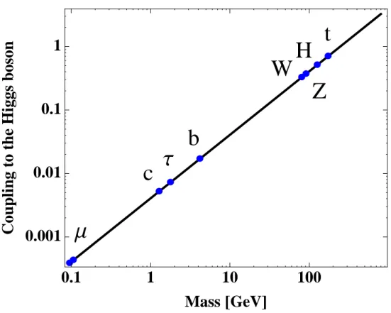
The important feature is that the Higgs couplings are controlled by the masses of the in- teracting particles. In particular, the couplings g_{h ¯f f},√g_{hhV V}/2 and√g_hhhh/3 are aligned on the linear line as we can see in the Fig. 1.

We can compute the decay widths of the Higgs boson to two vector bosons and two fermions; for the vector boson modes one vector boson is on-shell and the other is off-shell because m_h < 2mV. The results are the following:

Γ(h_{→ ¯}f f )_SM =

√2G_FN_c

8π ^m

2f^mh

√

1₋^4m

2f

m²_h ^{, (2.48)}

Γ(h_{→ W W}^∗)_SM = ^3α

2_m h

32 sin⁴θ_W^G ( m_W

m_h )

, (2.49)

Γ(h_{→ ZZ}^∗)_SM = ^α

2_m h

128π sin⁴θ_W(1_{− sin θW})² (

7₋⁴⁰

3 ^{sin θW +} 160

9 ^sin

2_θ W

)

G^{( mZ} m_h

) , (2.50) where N_c is the color factor, and we define the function G(x) as

G(x) =_{− |1 − x}²_|^{( 47} 2 ^x

2₋¹³

2 ⁺ 1 x²

)

− 3(1 − 6x^{2+ 4x4)}| ln x| + 3^{1− 8x + 20x}

4

√4x²_{− 1} ^arccos

( 3x²_{− 1} 2x³

)

. (2.51)

æ

æ æ

æ

æ

æ

æ^æ æ

H t

Z

W

b

c Τ

Μ

0.1 1 10 100

0.001

0.01

0.1

1

Mass @GeVD

Coupling to the Higgs boson

Figure 1. The strength of the Higgs coupling to other particles as a function of the masses of the interacting particles. The Higgs couplings are linearly dependent on the particle mass. A similar figure is seen in the Refs. [11,12].

2.2.2 One-loop level interactions

The quantum number of the Higgs field forbids the Higgs couplings with gg, γγ and Zγ at tree level. At loop level, however, the Higgs boson can decay into these particles. The loop induced decay modes are also important to clarify the Higgs properties; in some cases, the loop induced decays are fairly sensitive to new physics because the smallness of the SM effect leads to identifying easily a contribution from new physics.

First we consider the decay of the Higgs boson into two gluons. Since the gluon is SU (3)_c gauge boson, in the SM only the quarks appear in the loop; top and bottom quarks give large contribution to this process, and the other quarks are negligible due to their small masses, namely, small couplings to the Higgs boson. We here represent the formula including spin-0, 1/2 and 1 contributions for the sake of generality. The decay width is given by

Γ(h_{→ gg) =} ^α

s2^m3h

128π³    

δ_RT (V )^{ghV V}

m²_V ^{A1(τV) + δRT (f )} 2g_{h ¯f f}

m_f ^{A1/2(τf) + δRT (S)} g_hSS

m²_S ^A0(τS)    

2

. (2.52)

In the above the notation V ,f and S refer to spin-1, spin-1/2 and spin-0 particles, respec- tively. The loop functions are defined in the App.A, and the argument of the loop function is defined as τ_i = ^(2m_mⁱ

h

)2

. T (i) is the Dynkin index of the matter representation defined by the following relation on the group generators:

Tr[T^aT^b] = T (i)δ^ab. (2.53)

For SU (N ) fundamental representations and adjoint representations T (i) = ¹₂ and N , respectively. In addition, δR= ¹₂ for real matter fields and 1 otherwise. In the case of the SM, we can rewrite the coupling as

2g_{hf ¯f} m_f ⁼

2

v^{, (2.54)}

and the width becomes

Γ(h_{→ gg)SM} =

√2G_Fα²_sm³_h 128π³

A_1/2(τ_t) + A_1/2(τ_b)

2

∼ 2.0 × 10^{−4 [GeV], (2.55)}

where we use α_s= 0.119, m_t= 173 [GeV] and m_b = 4.8 [GeV].²

Next we provide the decay width of the Higgs boson into two photons. In this process the particles which get mass from the Higgs field and are electrically charged can enter the loop; W^±, quarks and charged leptons for the SM case. The decay width is expressed as

Γ(h_{→ γγ) =} ^α

2_m3 h

1024π³    

g_{hV V} m²_V ^Q

2V^A1^(τV^{) +}

2g_{h ¯f f} m_f ^Nc,fQ

2f^A1/2^(τf^{) +}

g_hSS m²_S ^Nc,SQ

2S^A0^(τS⁾

2

, (2.56) where Qi is the electric charge in |e| unit, Nc,i is the number colors for each particle. For the SM case

g_{hW W} m²_W ⁼

2g_{hf ¯f} m_f ⁼

2

v^{, (2.57)}

and the width is Γ(h_{→ γγ)SM} =

√2G_Fα²m³_h 256π³

1²A₁(τ_W) + 3^{( 2} 3

)2

A_1/2(τ_t) + 3^{( −1} 3

)2

A_1/2(τ_b)     

2

∼ 1.1 × 10^{−5 [GeV], (2.58)}

where we use α⁻¹ = 129 and m_W = 80.4 [GeV].

Finally we also consider the Higgs to Z photon decay mode. The particles appearing in the loop are the same as those of h → γγ. In this mode, however, there could be two particles with different masses inside the loop. Let us consider the case that the theory

2 Of course the QCD correction is significant in such a calculation, and we have to care about the renormalization scheme, see e.g. [13]. In this section we just put the pole mass into the equation.

includes the SM W^± boson and the fermions which are interacting with the Higgs boson and the Z boson with off-diagonal couplings in the mass eigenbasis. The Lagrangian is described as

L ⊃ m²W^Wµ^{+W−µ+ g}hW W^hWµ^+W−µ− mi^ψ¯i^ψi^{+ Q}i|e| ¯^ψi^γµψi^Aµ

− ¯^ψi^(cLij^PL^{+ cR}ij^PR^)ψj^{h + ¯ψ}i^γµ(λLij^PL^{+ λ}ij^RPR^)ψj^Zµ^{, (2.59)}

where P_L and P_R are the projection operators defined by P_L,R = ^1∓γ₂ ⁵. The decay width of this mode is expressed by the following:

Γ(h_{→ Zγ) =}^α

2_m3 h

512π³ (

1₋^m

2Z

m²_h )3

g_{hW W}

sin θ_Wcos θ_W^AV(mW) + ^2Nc

g sin θ_W

∑

i,j

Q_im_i(c^L_ij+ c^R_ij)(λ^L_ji+ λ^R_ji)A_F(m_i, m_j)      

2

. (2.60)

For the SM case we get Γ(h_{→ Zγ)SM} =

√2G_Fα²m³_h 128π³

( 1₋^m

2Z

m²_h )3

m²_W

sin θ_Wcos θ_W^AV(mW)

+ ^{2× 3}

sin θ_W cos θ_W {( 2

3 )

m²_t^{( 1}

2^{− 2 sin}

2_θ W ^{( 2}

3 ))

AF(mt, mt) + ^{( −1}

3 )

m²_b (

−¹

2^{− 2 sin}

2_θ

W^{( −1}

3 ))

A_F(m_b, m_b) }

2

∼7.0 × 10^{−6 [GeV]. (2.61)}

There doesn’t appear to be the off-diagonal contributions in the SM.

2.2.3 Experimental sensitivity to the Higgs couplings

It is important to precisely measure the Higgs couplings in order not only to confirm the SM, but also to investigate the physics beyond the SM. For the SM case, as we looked, the decay widths of the Higgs boson are determined by the mass of the particles and the EW parameters. The total decay width, Γ_H = ^∑_{all modes}Γ, is dependent on the Higgs mass and the result is shown in the Fig. 2. The total width sharply changes around the two vector boson threshold, and in the high mass region the width becomes too broad to be identified as a particle. For m_h = 126 [GeV], total width is Γ_H = 4.2_{× 10}⁻³ [GeV] which is too small to be experimentally measurable from the shape of the resonance.

The branching ratio (BR) for a particular decay mode is defined by Γ/Γ_H. The result of various modes is shown in the Fig.3. We can see the BR is sensitive to the Higgs mass. For m_h = 125.9 [GeV], the branching ratios are BR(bb) = 0.563, BR(W W^∗) = 0.229, BR(gg) = 0.0849, BR(τ τ ) = 0.0617, BR(ZZ^∗) = 0.0287, BR(cc) = 0.0284, BR(γγ) = 0.00228 and BR(Zγ) = 0.00162 [12]. Fortunately it is possible to measure various modes at the collider

[GeV] MH

100 200 300 1000

[GeV]HΓ

10-2

10-1

1 10 102

103

LHC HIGGS XS WG 2010

500

Figure 2. The total decay width as the function of the Higgs mass. The width is monotonic increasing with the Higgs mass. This figure is taken from the Refs. [14].

[GeV] MH

80 100 120 140 160 180 200

Higgs BR + Total Uncert

10-4

10-3

10-2

10-1

1

LHC HIGGS XS WG 2013

b b τ

τ

µ µ c c

gg

γ

γ Zγ

WW

ZZ

Figure 3. The branching ratio of the Higgs decay modes. In the light mass region (below the W W threshold) the main decay mode is bb. If the Higgs boson is sufficiently heavy the decay mode is dominated by W W and ZZ modes. This figure is taken from the Ref. [14].

experiments; the Higgs coupling is interesting target for the future physics.

Many studies of the Higgs coupling measurements are done. For example, the accura- cies that can be achieved by experiments at the LHC and at the ILC are estimated by the Refs. [15, 16]. The Fig. 4 show the 1σ experimental sensitivities to the Higgs couplings. At the LHC, due to the QCD back ground, the hbb and hτ τ couplings are difficult to be determined well. The loop induced couplings can be relatively well measured. Using ILC sensitivities, we can determine the couplings within 5% accuracy. Especially, tree level cou- plings, hV V and hbb, can be measured less than about 1%. Note that h→ Zγ mode has not studied yet although this process is as important as the other loop induced processes, h → gg and h → γγ; we need to study this mode and clarify its validity for the search of new physics.

-0.25 -0.2 -0.15 -0.1 -0.05 0 0.05 0.1 0.15

0 2 4 6 8 10

-0.25 -0.2 -0.15 -0.1 -0.05 0 0.05 0.1 0.15

0 2 4 6 8 10

-0.25 -0.2 -0.15 -0.1 -0.05 0 0.05 0.1 0.15

0 2 4 6 8 10

-0.25 -0.2 -0.15 -0.1 -0.05 0 0.05 0.1 0.15

0 2 4 6 8 10

-0.25 -0.2 -0.15 -0.1 -0.05 0 0.05 0.1 0.15

0 2 4 6 8 10

-0.25 -0.2 -0.15 -0.1 -0.05 0 0.05 0.1 0.15

0 2 4 6 8 10

-0.25 -0.2 -0.15 -0.1 -0.05 0 0.05 0.1 0.15

0 2 4 6 8 10

-0.25 -0.2 -0.15 -0.1 -0.05 0 0.05 0.1 0.15

0 2 4 6 8 10

-0.25 -0.2 -0.15 -0.1 -0.05 0 0.05 0.1 0.15

0 2 4 6 8 10

-0.25 -0.2 -0.15 -0.1 -0.05 0 0.05 0.1 0.15

0 2 4 6 8 10

-0.25 -0.2 -0.15 -0.1 -0.05 0 0.05 0.1 0.15

0 2 4 6 8 10

-0.25 -0.2 -0.15 -0.1 -0.05 0 0.05 0.1 0.15

0 2 4 6 8 10

-0.25 -0.2 -0.15 -0.1 -0.05 0 0.05 0.1 0.15

0 2 4 6 8 10

-0.25 -0.2 -0.15 -0.1 -0.05 0 0.05 0.1 0.15

0 2 4 6 8 10

-0.25 -0.2 -0.15 -0.1 -0.05 0 0.05 0.1 0.15

0 2 4 6 8 10

-0.25 -0.2 -0.15 -0.1 -0.05 0 0.05 0.1 0.15

0 2 4 6 8 10

-0.25 -0.2 -0.15 -0.1 -0.05 0 0.05 0.1 0.15

0 2 4 6 8 10

-0.25 -0.2 -0.15 -0.1 -0.05 0 0.05 0.1 0.15

0 2 4 6 8 10

-0.25 -0.2 -0.15 -0.1 -0.05 0 0.05 0.1 0.15

0 2 4 6 8 10

-0.25 -0.2 -0.15 -0.1 -0.05 0 0.05 0.1 0.15

0 2 4 6 8 10

-0.25 -0.2 -0.15 -0.1 -0.05 0 0.05 0.1 0.15

0 2 4 6 8 10

-0.25 -0.2 -0.15 -0.1 -0.05 0 0.05 0.1 0.15

0 2 4 6 8 10

-0.25 -0.2 -0.15 -0.1 -0.05 0 0.05 0.1 0.15

0 2 4 6 8 10

-0.25 -0.2 -0.15 -0.1 -0.05 0 0.05 0.1 0.15

0 2 4 6 8 10

-0.25 -0.2 -0.15 -0.1 -0.05 0 0.05 0.1 0.15

0 2 4 6 8 10

-0.25 -0.2 -0.15 -0.1 -0.05 0 0.05 0.1 0.15

0 2 4 6 8 10

-0.25 -0.2 -0.15 -0.1 -0.05 0 0.05 0.1 0.15

0 2 4 6 8 10

-0.25 -0.2 -0.15 -0.1 -0.05 0 0.05 0.1 0.15

0 2 4 6 8 10

-0.25 -0.2 -0.15 -0.1 -0.05 0 0.05 0.1 0.15

0 2 4 6 8 10

-0.25 -0.2 -0.15 -0.1 -0.05 0 0.05 0.1 0.15

0 2 4 6 8 10

-0.25 -0.2 -0.15 -0.1 -0.05 0 0.05 0.1 0.15

0 2 4 6 8 10

-0.25 -0.2 -0.15 -0.1 -0.05 0 0.05 0.1 0.15

0 2 4 6 8 10

-0.25 -0.2 -0.15 -0.1 -0.05 0 0.05 0.1 0.15

0 2 4 6 8 10

-0.25 -0.2 -0.15 -0.1 -0.05 0 0.05 0.1 0.15

0 2 4 6 8 10

-0.25 -0.2 -0.15 -0.1 -0.05 0 0.05 0.1 0.15

0 2 4 6 8 10

-0.25 -0.2 -0.15 -0.1 -0.05 0 0.05 0.1 0.15

0 2 4 6 8 10

-0.25 -0.2 -0.15 -0.1 -0.05 0 0.05 0.1 0.15

0 2 4 6 8 10

-0.25 -0.2 -0.15 -0.1 -0.05 0 0.05 0.1 0.15

0 2 4 6 8 10

W Z b g γ τ c t inv.

g(hAA)/g(hAA)| _SM -1 LHC/ILC1/ILC/ILCTeV

Figure 4. Comparison of the capabilities of the LHC and the ILC model independent measure- ments of the Higgs couplings. The plot shows (from left to right in each set of error bars) 1 σ confidence intervals for LHC at 14 [TeV] with 300 [fb⁻¹], for ILC at 250 [GeV] and 250 [fb⁻¹] (‘ILC1’), for the full ILC program up to 500 [GeV] with 500 [fb⁻¹] (‘ILC’), and for a program with 1000 [fb⁻¹] for an upgraded ILC at 1 [TeV] (‘ILCTeV’). The marked horizontal band represents a 5% deviation from the Standard Model prediction for the coupling. This figure is taken from the Ref. [15].

2.3 Theoretical aspects of Higgs physics

In this section we provide several theoretical aspects of Higgs physics. The Higgs field is introduced as the only scalar field in the SM to cause the EW symmetry breaking. Therefore, its theoretical properties are various and important to understand what the Higgs field is. They are also useful to investigate new physics because models with extended Higgs sector likely modify the properties.

2.3.1 Perturbative unitarity

In this subsection we discuss the perturbative unitarity of the scattering amplitudes. The amplitudes of elastic scattering satisfy the following relation for each partial wave:

M_n^I =λ(a, b)M_n^R+ iM_n^I

2, (2.62)

λ(a, b) =√(1 − (a + b)²⁾⁽¹− (a − b)^{2), (2.63)} where M_n^R(M_n^I) is the real (imaginary) part of the partial wave amplitude, a and b are the ratios between the mass of each particle and the center of mass energy, m_a,b/^√s, and partial waves are defined as below with the Legendre polynomials Pm(x):

M(cos θ) = 16π

∑∞ n=0

(2n + 1)M_nP_n(cos θ), (2.64)

∫ ₁

−1

dx P_m(x)P_n(x) = ²

2n + 1^{δmn. (2.65)}

Eq. (2.62) is the equation of the circle with radius _2λ¹ and center (0,_2λ¹ ). In the high- energy limit where the masses of produced particles can be neglected, the radius of the circle becomes the maximum. Therefore, the actual amplitudes are in the maximal circle. Finally, partial wave amplitudes at least satisfy M_n^R _{∈ [−}¹₂,¹₂] and M_n^I ∈ [0, 1]. If we consider processes involving identical particles in the final state, the bound becomes weaker as M_n^R∈ [−1, 1] and Mn^I ∈ [0, 2].

As an example, let us consider the two-body to two-body scattering amplitudes of the longitudinal gauge bosons. The polarization vector of the massive gauge boson is expressed as

ϵ^µ_L= ^E m_V

(|p| Ep

|p|

)

, (2.66)

where E and p are energy and three momentum, respectively. Naive estimation of a two body to two body scattering amplitude is then

M(VL^aVL^b → VL^cVL^d)∝ |ϵ^µ_L|⁴

∼ ^E

4

m⁴_V^{. (2.67)}

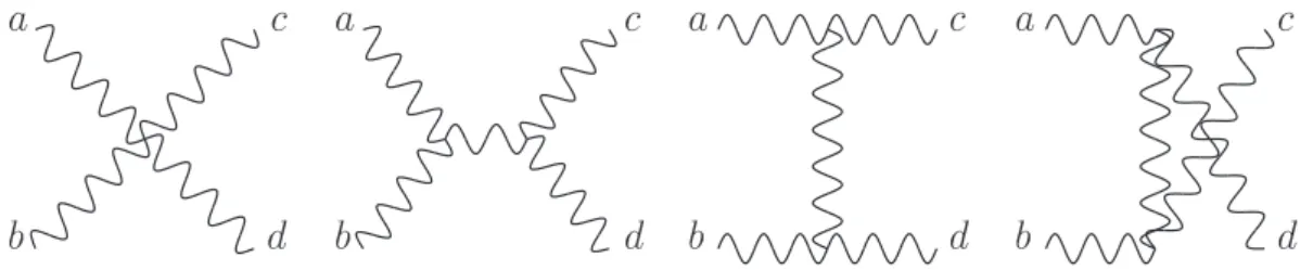
This amplitude seems to be divergent in the ultraviolet region. First we consider the process of longitudinal gauge boson two-body to two-body scatterings with g^′ = 0 case. Diagrams including only the gauge bosons are comprised of one with four point interaction and ones with three point interaction.

a

b

d a

b

d a

b

d a

b

d

Figure 5. Two-body to two-body scattering process of longitudinal gauge bosons, including only the gauge bosons. Indices, a, b, c and d, denote the component of the gauge boson.

Focusing on the contributions which diverse as energy increases, we can write the amplitude of the four point interaction diagram as

M4^(ab→ cd) = gW W W W

E⁴ m⁴_W

(

−6 + 2 cos^{2θ + 4m}

2W

E² )

δ^abδ^cd+_{· · · .} (2.68)

The t-channel and u-channel contributions are Mt(ab_{→ cd) = g}²_{W W W} ^E

4

m⁴_W (

3− 2 cos θ − cos^{2θ +} (

−³ 2 ⁺

15 2 ^{cos θ}

) m²_W E²

)

δ^abδ^cd+_{· · · ,} (2.69) Mt^(ab→ cd) = g²W W W

E⁴ m⁴_W

(

3 + 2 cos θ_{− cos}²θ + (

−³₂ −¹⁵₂ ^{cos θ) m}

2W

E² )

δ^abδ^cd+_{· · · .} (2.70) Note that s-channel contribution to this term vanishes due to the nature of the structure constant. The gauge symmetry guarantees the following relation:

g_{W W W W} = g_{W W W}² = g². (2.71)

Thanks to this relation the sum of these contribution becomes M4⁺Mt⁺Mu ^{= g2}

E² m²_W^δ

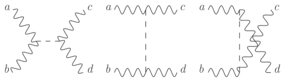
ab_δcd_{, (2.72)}

We can see E⁴ dependence vanishes. The E² dependence, however, still remains and violates the tree level unitarity in the high energy region. The Higgs boson mediated diagram, see the Fig.6, plays an crucial role to save this difficulty.