On the nonstationarity of the exchange rate process
Takaaki Ohnishi
a,b,⁎ , Hideki Takayasu
c, Takatoshi Ito
b, Yuko Hashimoto
d,
Tsutomu Watanabe
a,e, Misako Takayasu
faThe Canon Institute for Global Studies, 11F, Shin-Marunouchi Bldg., 1-5-1, Marunouchi, Chiyoda-Ku, Tokyo 100-6511, Japan
bGraduate School of Economics, University of Tokyo, 7-3-1 Hongo, Bunkyo-Ku, Tokyo, 113-0033, Japan
cSony Computer Science Laboratories, 3-14-13 Higashigotanda, Shinagawa-ku, Tokyo, 141-0022, Japan
dStatistics Department, International Monetary Fund, 700 19th Street, N.W., Washington, D.C. 20431, United States
eInstitute of Economic Research, Hitotsubashi University, 2-1 Naka, Kunitachi-city, Tokyo 186-8603, Japan
fDepartment of Computational Intelligence and Systems Science, Interdisciplinary, Graduate School of Science and Engineering, Tokyo Institute of Technology, 4259-G3-52, Nagatsuta-cho, Midori-ku, Yokohama 226-8502, Japan
a b s t r a c t a r t i c l e i n f o
Article history:
Received 15 November 2010 Received in revised form 10 May 2011 Accepted 30 June 2011
Available online xxxx
Keywords: Econophysics
Foreign exchange market Strict stationarity Nonstationarity
Two-sample Kolmogorov–Smirnov test Pearson's chi-square test
Poisson process
We empirically investigate the nonstationarity property of the USD–JPY exchange rate by using a high frequency data set spanning 8 years. We perform a statistical test of strict stationarity based on the two-sample Kolmogorov–Smirnov test for the absolute price changes, and Pearson's chi square test for the number of successive price changes in the same direction, and find statistically significant evidence of nonstationarity. Further, we study the recurrence intervals between the days in which nonstationarity occurs and find that the distribution of recurrence intervals is well approximated by an exponential distribution. In addition, we find that the mean conditional recurrence interval hTjT0i is independent of the previous recurrence interval T0. These findings indicate that the recurrence intervals are characterized by a Poisson process. We interpret this observation as a reflection of the Poisson property regarding the arrival of news.
© 2011 Elsevier Inc. All rights reserved.
1. Introduction
In econophysics, financial time series data have been extensively investigated using a wide variety of methods. These studies tend to assume, explicitly or implicitly, that a time series is stationary, since stationarity is a requirement for most of the mathematical theories underlying time series analysis. However, despite its nearly universal assumption, few previous studies seek to test stationarity in a reliable manner (Tóthla, et al., 2010).
For low-frequency financial data (i.e., monthly or daily data), a number of procedures to test stationarity have been advocated and applied to various time series processes in econometrics. Most of them focus on the first two moments of a process; in other words, they test covariance stationarity. These tests work well for normally distributed random variables. However, for high-frequency financial data such as tick-by-tick data, it is well known that price change distributions are fat-tailed and substantially deviate from a normal
distribution. These fat-tailed distributions cannot be dealt with by the above stationarity tests.
In this paper, we advocate a test for strict stationarity that considers the entire distribution of a process rather than the first two moments of the process, and apply this test to the USD–JPY exchange rate.
We describe the data used in this paper inSection 2. InSection 3, we explain our procedure to test stationarity, which is based on the two-sample Kolmogorov–Smirnov test and Pearson's chi-square test. InSection 4, we present the empirical results. InSection 5, we discuss some implications of our results.
2. Data description
The tick-by-tick data we study is the USD–JPY exchange rate provided by ICAP EBS with a recording frequency of every 1 s, for the period of January 1998 through December 2005. The foreign exchange market is the world's largest and liquid financial market. Most spot interbank transactions are executed through global electronic broking systems such as ICAP EBS and Reuters. In the USD–JPY exchange rate, the ICAP EBS has a strong market share.
We exclude observations for special days such as Mondays, weekends, holidays, and official intervention days (i.e., the government International Review of Financial Analysis xxx (2011) xxx–xxx
⁎Corresponding author at: The Canon Institute for Global Studies, 11F, Shin- Marunouchi Bldg., 1-5-1, Marunouchi, Chiyoda-Ku, Tokyo 100-6511, Japan.
E-mail address:ohnishi.takaaki@canon-igs.org(T. Ohnishi). FINANA-00474; No of Pages 5
1057-5219/$ – see front matter © 2011 Elsevier Inc. All rights reserved. doi:10.1016/j.irfa.2011.06.010
Contents lists available atScienceDirect
International Review of Financial Analysis
and/or the central bank intervenes in the foreign exchange market in order to stabilize the rate), which are obviously different from regular business days. We analyze the time series of 1-tick price changes of the mid-quote price, which is defined as the average of the best bid and the best ask. The best bid and the best ask, representing the lowest sell offer and highest buy offer respectively, are recorded at the end of one- second time slice.
In this paper, we focus on the following two time series: The first one is the time series for the absolute price changes, which we refer to as G; second, the time series for the number of successive price changes in the same direction, which we refer to as D. Note that in producing these time series, we drop observations with no price changes. For example, a particular sequence of 14 1-tick price changes
f0:01;0:02;0:01;−0:02;0;−0:03;−0:01;0:02;0;0:02;−0:04;0:01;
−0:02;−0:03g
is represented by
f0:01;0:02;0:01;0:02;0;0:03;0:01;0:02;0;0:02;0:04;0:01;0:02;0:03;g
in G sequence and
f3; 3; 2; 1; 1; 2g
in D sequence.
3. Stationarity test
One can test stationarity in Gaussian time series processes by measuring any number of simple statistics such as the mean or standard deviation and employing a standard statistical test. However, such an approach is not particularly effective for high-frequency financial time series, because from the seminal work byMantegna and Stanley(1995), we know that the distributions of price changes have fat tails often approximated by a power law (Ohnishi et al., 2008). Therefore, the procedure for Gaussian processes cannot be applied to high-frequency financial data.
Our analysis is based on a precise definition of stationarity: The joint distribution of any two segments of data of the same length should be identical. Formally, a stochastic process Xtis called strictly stationary if for any set of times t1, t2, …, tnand for any k, the joint probability distributions of {Xt1, Xt2, …, Xtn} and of {Xt1+ k, Xt2+ k, …, Xtn+ k} coincide. That is, it requires that the joint distribution depends only on time lags. It follows that the mean remains constant, and that the autocorrelation function depends on only time lags, and not on the time index.
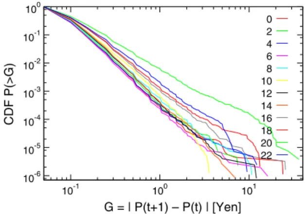
Given this definition of stationarity, the test of stationarity may look straightforward: namely, all we have to do is to pick up any two segments of data of the same length, and then to see whether the distributions of G and D are identical across the two segments. However, the test of stationarity is not so simple since the exchange rate exhibits a strong seasonality. It is well known by practitioners and researchers that trading occurs differently even within a day, depending on, for instance, whether it is conducted in the morning or afternoon session. Specifically, we know from the previous studies that the absolute price changes (Ohnishi et al., 2008) and activities (Ito & Hashimoto, 2006) display an intraday seasonality.Figs. 1 and 2 present the cumulative distributions of G and D respectively, showing clearly that these distributions differ depending on the hour of the day.
One may want to apply some traditional methods of seasonal adjustment, such as X-12-ARIMA, in order to eliminate this intraday seasonality. However, such methods may not be appropriate in this context, since the time series property of G and D may be altered substantially by applying these methods. To avoid such risk, we eliminate the intraday seasonality in a different way. First, we assume
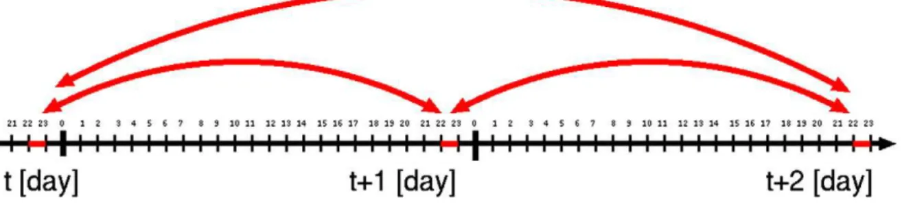
that the time series can be regarded as approximately stationary at least during the one-hour period. Second, on the basis of this assumption, we divide the entire time series into the subsets with one-hour periods, each of which is identified by hour h = 0, 1,…, 23 and day t. Third, we compare the distributions of G and D for the subset (h, t) (i.e., the set of observations belonging to hour h of day t) with those for the subset (h, t′) (i.e., the set of observations belonging to hour h and day t′), as illustrated schematically inFig. 3. Note that we compare the observations belonging to the same hour h, although they come from different days. In this way, we conduct the stationarity test separately for each h (h = 0, 1, …, 23).
To test for stationarity, we compare the distribution of observations belonging to the subset (h, t) and that belonging to the subset (h, t′) to examine whether the two distributions are identical. We perform tests by using the two-sample Kolmogorov–Smirnov test for continuous distributions of G and Pearson's chi-square test for discrete distributions of D. The stationarity is determined at a conventional significance level of 5%. The two-sample Kolmogorov–Smirnov test compares two cumulative distribution functions of G; then, the maximum difference between these two cumulative distribution functions yields the P-value. Pearson's chi-square test is performed by considering a histogram of D having 4 bins, that is, D =1, D = 2, D = 3, and D ≥ 4. These two tests have the advantage of being nonparametric, and without making assumptions about the distribution function of the data, we get the probability that the two sets of data are drawn from the same distribution.
10-6 10-5 10-4 10-3 10-2 10-1 100
10-1 100 101
CDF P(>G)
G = | P(t+1) – P(t) | [Yen] 0 2 4 6 8 10 12 14 16 18 20 22
Fig. 1. Cumulative probability distributions of absolute price changes G. The colors represent the different hours of the day.
2 4 6 8 10 12 14 16
CDF P(>D)
D 1 / 2D-1
0 2 4 6 8 10
12 14 16 18 20 22
10-6 10-5 10-4 10-3 10-2 10-1 100
Fig. 2. Cumulative probability distributions of the number of successive price changes in the same direction D. The colors represent the different hours of the day. T. Ohnishi et al. / International Review of Financial Analysis xxx (2011) xxx–xxx
4. Results
First, we compare the distribution of observations in the subsets (h, t) and (h, t′) for every pair of t and t′. This exercise is repeated N0∼106 times. Then, we count the number of times, which is denoted by N, in which we reject the null hypothesis that the two distributions are identical.Fig. 4shows the results of this exercise. The y-axis represents N/N0. Note that if the entire time series is stationary, the rejection rate would be 5%. The x-axis represents the hour of the day. The closed symbols represent the result of this exercise for G; the open symbols, for D. We see that for each h, the rejection rate is much higher than the critical value, that is, 5%, indicating that the null hypothesis of stationarity is clearly rejected. We suspect that this is the result of long time correlations in the time series of the absolute value of price changes (volatility clustering). Turning to the results for D, we again find that for each h, the rejection rate is significantly above the critical value. Therefore, we conclude from these exercises that the exchange rate process is not a stationary process.
Next, we repeat the same test, but this time we compare observations in the subsets (h, t) and (h, t + τ) for different values of τ.Fig. 5shows the results of this exercise. The y-axis represents the rejection rate, which is averaged over different h and t. The x-axis represents time lags τ. The closed symbols are the results for G. For τ= 1 day, as many as 34% of the results are nonstationary. This number rises to more than 45% for τ ≥ 60 days. The open symbols are the results for D, showing similar features. For τ = 1 day, as many as 18% are nonstationary. The percentage monotonically increases as the time lag τ increases. As the time lag increases, there are more opportunities for different distributions to emerge, and stationarity is lost.
For a more detailed investigation of the properties of nonstationarity, we focus on the interval between the days in which nonstationarity
occurs. Specifically, we compare observations in the subsets (h,t) and (h, t + 1) to see whether the distributions of G (or D) differ between t and t + 1. We repeat this for each t, thereby identifying the days in which nonstationarity occurs. We denote them by ti, where i =1,2,…. Then we define recurrence interval {T} as ti−ti − 1. The cumulative probability distributions as functions of the scaled recurrence intervals T/〈T〉 are shown inFigs. 6 and 7for G and D respectively. For each hour of the day, these distributions follow an exponential distribution, where 〈T〉 is about 10 days for G and 3 days for D.
The independence of T is also verified in the mean conditional interval 〈Ti + 1|Ti〉, which is defined as the mean of recurrence intervals Ti + 1conditional on the preceding interval Tias shown inFig. 8, where we plot 〈Ti + 1|Ti〉/〈T〉 as a function of Ti + 1/〈T〉. Clearly, for both G and D,
〈Ti + 1|Ti〉/〈T〉 fluctuates around a horizontal line close to 1, indicating that Ti + 1is independent of the previous Ti. Thus, there is no memory effect in the recurrence intervals. The numbers of occurrences counted in disjoint periods are independent from each other (i.e., independent increments).
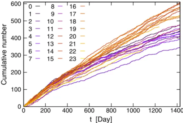
Finally,Figs. 9 and 10show the cumulative number of occurrence of nonstationarity up to time t days. For both G and D, the cumulative number exhibits an almost linear increase; that is, the slope of the cumulative number is constant. Thus, the probability distribution of the number of occurrences, counted in any time period depends on only the length of the period (i.e., stationary increments).
In sum, we have found that the occurrence of nonstationarity possesses the following properties: Poisson distribution of the recurrence intervals, independent increments, and stationary in- crements. Hence, the occurrence of nonstationarity is well modeled by the Poisson process. Nonstationarities occur at random instants of time at an average rate of λ per day, where λ = 1/〈T〉 is about 0.1 for G and 0.33 for D.
Fig. 3. Comparison of two sub-series on the same hour of different days.
0 10 20 30 40 50 60
0 4 8 12 16 20 24
N/N0 [%]
Hour G
D
Fig. 4. Percentage of all pairs whose difference lies beyond the expected value at a 5 percent significance level. Closed symbols give the results for G; open symbols, for D. This percentage is greater than 5%, displaying clear evidence of nonstationarity.
16 24 32 40 48
100 101 102
N/N0 [%]
τ [Day] G
D
Fig. 5. Percentage of all pairs whose difference lies beyond the expected value at a 5 percent significance level. Closed symbols give the results for G; open symbols, for D. This percentage increases with the time lag τ, suggesting that the data become more nonstationary as the time lag increases.
T. Ohnishi et al. / International Review of Financial Analysis xxx (2011) xxx–xxx
5. Discussion
We have studied the time series of the absolute price changes and the number of successive price changes in the same direction. First, by testing nonstationarity of the time series on the basis of the two-sample Kolmogorov–Smirnov test and Pearson's chi-square test, we have found that both the absolute price changes and the number of successive price changes deviate substantially from a stationary process. Second, we have investigated the properties of nonstationarity and have found that the recurrence intervals between the days in which nonstationarity occurs are modeled by the Poisson process.
For the absolute price changes, long-term correlations are likely to reflect nonstationarity. However, the origin of nonstationarity might differ from the long-term memory of the volatility, because our observations of the recurrence intervals disagree with the results reported by previous studies that were based on the return intervals between price volatility above a certain threshold, where the return intervals strongly depend on the previous return interval (Yamasaki et al., 2005; Wang et al., 2007, 2006; Vodenska-Chitkushev et al., 2008; Jung et al., 2008).
The results for the number of successive price changes are very interesting, because the number depends not on the size of price changes, but on the signs of these changes. Although previous papers have found some evidence for the presence of the memory effect in the sign of price changes (Mizuno et al., 2003; Hashimoto et al., 2008), the length of memory reported in those papers is several tens of
seconds, which is clearly too short-lived to account for the nonstationarity observed in the previous section.
The average recurrence intervals for the absolute price changes are larger than those for the number of successive price changes. In other words, non-stationarity is more prominent in the signs, rather than the size, of price changes. Currently, the reason for this feature is not clear. This will be a subject of further study.
Despite both time series capturing different features of price changes, the recurrence intervals of nonstationarity are characterized
0 1 2 3 4 5 6 7 8
CDF P(>T)
T / < T > 10-2
10-1 100
Fig. 6. Cumulative probability distributions of recurrence intervals T for G. The colors represent the different hours of the day. The straight line is for demonstration, and has a slope of −1.
0 1 2 3 4 5 6 7 8
T / < T >
CDF P(>T)
10-2 10-1 100
Fig. 7. Cumulative probability distributions of recurrence intervals T for D. The colors represent the different hours of the day. The straight line is for demonstration, and has a slope of −1.
0.1 0.2 0.5 1 2
0.1 1 10
< Ti+1 | Ti > / < T >
Ti / < T > G
D
Fig. 8. Scaled mean conditional interval 〈Ti + 1|Ti〉/〈T〉 as a function of scaled preceding interval Ti + 1/〈T〉. Closed symbols give the results for G; open symbols for D.
0 100 200 300 400 500 600
0 200 400 600 800 1000 1200 1400
Cumulative number
t [Day] 0
1 2 3 4 5 6 7
8 9 10 11 12 13 14 15
16 17 18 19 20 21 22 23
Fig. 9. The cumulative number of occurrence of nonstationarity for G. The colors represent the different hours of the day. Almost linear increases suggest nonhomoge- neous Poisson process.
0 20 40 60 80 100 120 140 160
0 200 400 600 800 1000 1200 1400
Cumulative number
t [Day] 0
1 2 3 4 5 6 7 8 9 10 11
12 13 14 15 16 17 18 19 20 21 22 23
Fig. 10. The cumulative number of occurrence of nonstationarity for D. The colors represent the different hours of the day. Almost linear increases suggest nonhomoge- neous Poisson process.
T. Ohnishi et al. / International Review of Financial Analysis xxx (2011) xxx–xxx
by the Poisson process for both cases. Therefore, the most possible explanation for nonstationarity is the arrival of news, which is considered to be well described by the Poisson process. The efficient market hypothesis claims that prices reflect all news coming into the markets very rapidly. Possibly, the nonstationarity of price changes is a reflection of the nonstationarity of the arrival of news.
Nonstationarity poses a serious problem for the calculation of the auto-correlation function of the time series. The correlation co- efficients themselves may not be constant, which leads to an unexpected estimation error. These findings could lead to a better understanding and modeling of the price dynamics.
Acknowledgments
Numerical calculations were performed by using the Hitachi HA8000 at the Information Technology Center, University of Tokyo. T.O. acknowledges the grant from the Ministry of Education, Culture, Sports, Science, and Technology of Japan (Grant-in-Aid for Young Scientists (A) No. 23686019).
References
Hashimoto, Y., Ito, T., Ohnishi, T., Takayasu, M., Takayasu, H., & Watanabe, T. (2008). NBER Working Paper.
Ito, T., & Hashimoto, Y. (2006). Journal of the Japanese and International Economies, 20, 637–664.
Jung, W., Wang, F., Havlin, S., Kaizoji, T., Moon, H., & Stanley, H. (2008). The European Physical Journal B, 62, 113–119.
Mantegna, R., & Stanley, H. (1995). Nature, 376, 46–49.
Mizuno, T., Kurihara, S., Takayasu, M., & Takayasu, H. (2003). Physica A: Statistical Mechanics and its Applications, 324, 296–302.
Ohnishi, T., Takayasu, H., Ito, T., Hashimoto, Y., Watanabe, T., & Takayasu, M. (2008). Journal of Economic Interaction and Coordination, 3, 99–106.
B. Tóthla, F. Lillo, J. Farmer, arXiv:1001.2549v1 (2010).
Vodenska-Chitkushev, I., Wang, F., Weber, P., Yamasaki, K., Havlin, S., & Stanley, H. (2008). The European Physical Journal B—Condensed Matter and Complex Systems, 61, 217–223.
Wang, F., Weber, P., Yamasaki, K., Havlin, S., & Stanley, H. (2007). The European Physical Journal B—Condensed Matter and Complex Systems, 55, 123–133.
Wang, F., Yamasaki, K., Havlin, S., & Stanley, H. (2006). Physical Review E, 73, 26117. Yamasaki, K., Muchnik, L., Havlin, S., Bunde, A., & Stanley, H. (2005). Proceedings of the
National Academy of Sciences, 102, 9424–9428. T. Ohnishi et al. / International Review of Financial Analysis xxx (2011) xxx–xxx