THE JOURNAL OF FINANCE•VOL. LXXII, NO. 4•AUGUST 2017
Selling Failed Banks
JO ˜AO GRANJA, GREGOR MATVOS, and AMIT SERU∗
ABSTRACT
The average FDIC loss from selling a failed bank is 28% of assets. We document that failed banks are predominantly sold to bidders within the same county, with similar assets business lines, when these bidders are well capitalized. Otherwise, they are acquired by less similar banks located further away. We interpret these facts within a model of auctions with budget constraints, in which poor capitalization of some potential acquirers drives a wedge between their willingness and ability to pay for failed banks. We document that this wedge drives misallocation, and partially explains the FDIC losses from failed bank sales.
THE GREAT RECESSION and its aftermath saw an unprecedented number of banks being taken into receivership by the Federal Deposit Insurance Corpo-ration (FDIC) and then sold at auction. These failures impose substantial costs on the FDIC: the average cost of a failed bank sold at auction over the 2007 to 2013 period was approximately 28% of the failed bank’s assets. The resolution of bank failures led to Deposit Insurance Fund (DIF) costs of approximately $90 billion, leaving the fund with a negative balance of almost $21 billion at the height of the crisis in 2009 (Davison and Carreon (2010)). Small and medium-sized banks, which are typically sold at FDIC auctions, have also been large beneficiaries of government programs during this period.1 For example, the Treasury department does not expect to recover all of the $791 million of Trou-bled Asset Relief Program (TARP) funds that were awarded to 26 failed banks in our sample (Office of the Special Inspector General for the Troubled Asset Relief Program (2014)). In spite of the importance of failed bank resolutions during the recent crisis, little is known about the allocation of failed banks since the Savings & Loans (S&L) crisis (James and Wier (1987), James (1991)).
∗Jo ˜ao Granja is with the Booth School of Business, University of Chicago. Gregor Matvos is with the Booth School of Business, University of Chicago and NBER. Amit Seru is with Stanford GSB, Stanford University, and NBER. We thank Sumit Agarwal; Charlie Calomiris; Douglas Diamond; Mark Flannery; Chris James; Anil Kashyap; Christian Leuz; Elena Loutskina; Toby Moskowitz; Enrico Perotti; Michael Roberts (the Editor); Phil Strahan; Amir Sufi; Rob Vishny; seminar partic-ipants at Becker Friedman Institute Conference on Creditors and Corporate Governance, Becker Brownbag, Chicago Booth (Accounting and Finance), Federal Reserve, MIT Sloan, NBER Risk of Financial Institutions Summer Meeting, and Washington University Conference on Corporate Finance for helpful suggestions. The authors have no conflict of interest to declare. All errors are our own.
1State chartered banks, which constitute 65% of failed banks in our sample, received
approxi-mately $50 billion of TARP funds to help them absorb liquidity shortfalls during the financial crisis. The banks in our sample account for 80% of losses to the Deposit Insurance Fund (see Appendix Figure A.2). The Internet Appendix may be found in the online version of this article.
DOI: 10.1111/jofi.12512
We study whether the allocation of failed banks during the Great Recession was distorted because potential acquirers of these banks were poorly capital-ized. We do so within a model of auctions with budget constraints. In our model, poor capitalization of some potential acquirers drives a wedge between their willingness and ability to pay for a failed bank. This wedge leads to a potential misallocation of failed banks. Using our framework, we identify three charac-teristics that drive potential acquirers’ willingness to pay for a failed bank in the data. We find that the bidding behavior of poorly capitalized acquirers is consistent with the predictions of our model. We further find that the wedge be-tween potential acquirers’ willingness and ability to pay distorts the allocation of failed banks. The costs of this misallocation are substantial, as measured by the additional resolution costs of the FDIC. This paper is the first to study the qualitative and quantitative allocation consequences of failed bank sales.
We begin by identifying three characteristics of potential acquirers that drive their willingness to pay for a failed bank. A prediction of our model is that potential acquirers that value the failed bank more are more likely to win the failed bank auction. Therefore, if we observe that certain potential acquirers are more likely to win an auction, we can infer that they value the bank more than other potential acquirers. We show that local banks are by far the most likely acquirers of failed banks: only about 15% of failed banks are sold to a bank that does not currently have branches within the same state, and more than one-third of failed banks are sold to a bank that has at least one branch in the same zip code. We thus find that a geographically proximate bank is significantly more likely to acquire a failed bank. This result is robust to the inclusion of failed bank fixed effects and potential acquirer-quarter fixed effects, which implies that the documented effect is driven not by the inherent quality of the failed bank or the acquirer but rather by the relative distance between the branch networks of the failed banks and the acquirer. Our evidence is not consistent with the idea that information technology and integration in banking markets have eliminated the advantage of local banks and allowed geographically distant banks to acquire failed banks (Cochrane (2013)).
One potential reason geographically proximate potential acquirers are will-ing to pay more for a failed bank is that they have access to better soft in-formation. Consistent with the idea that valuable soft information decreases with geographic distance, we find that, in regions with more soft information, acquisitions of failed banks by local banks are more likely. In these regions, the willingness to pay for a failed bank decreases faster with distance.
Selling Failed Banks 1725
offers similar services. Failed bank and acquirer-quarter fixed effects ensure that these results are not driven by inherent characteristics of the failed bank or potential acquirer but rather by the relative similarity between the portfolio composition of and services offered by potential acquirers and failed bank. The effects we document are economically meaningful. For instance, the likelihood of acquisition declines by one-third of the mean if a potential acquirer’s CRE portfolio share distance from the failed bank differs by one standard deviation. A third characteristic that affects potential acquirers’ willingness to pay for a failed bank is the increase in market concentration resulting from an acquisition. Potential acquirers whose market concentration increases most with the acquisition of the failed bank should have a higher willingness to pay for a failed bank and thus should be most likely to acquire the failed bank. We find an economically small but statistically significant effect of market concentration.
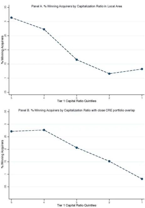
After documenting the above characteristics affecting a potential acquirer’s willingness to pay for a failed bank, we examine whether the capitalization of potential acquirers impacts their ability to pay for a failed bank. We find a monotonic relationship between the capitalization of potential local acquirers and their propensity to acquire failed banks: the 20% best capitalized local buyers acquire over 30% of failed banks, while the 20% most poorly capitalized local buyers acquire only 10% of failed banks.
Our framework suggests that if poor capitalization hinders a potential ac-quirer’s ability to bid for a bank, poorly capitalized acquirers may lose to better capitalized banks who value the failed bank less. We confirm this prediction in the data. When local potential acquirers are poorly capitalized, the failed bank is more likely to be acquired by a distant acquirer, one with a lower willing-ness to pay for the failed bank. Similarly, potential acquirers in related lines of business are most likely to acquire a failed bank if they are well capital-ized. We find that low capitalization of these buyers forces the sale of a failed bank to acquirers in less related lines of business. A failed bank is also sold to acquirers with smaller market concentration gains if potential acquirers that would increase market concentration most are poorly capitalized. As before, we obtain these results after accounting for failed bank and acquirer-quarter fixed effects, which implies that the results are not driven by inherent failed bank or potential acquirer characteristics. Overall, the results suggest that the low capitalization of potential acquirers distorts the allocation of failed banks toward acquirers with lower valuations.
Two broad channels can explain the results on failed bank allocation. Under our framework, failed bank allocation is driven by potential acquirers’ willing-ness and ability to pay. A bank acquires a failed bank because it chooses to bid more for the failed bank than other potential acquirers, which either bid less or choose not to participate in the bidding process. Under the alternative, the FDIC chooses which banks are allowed to bid in an auction through its eligibility criteria, and it is these criteria that affect failed bank allocation.
constrain our sample to actual acquirers that have been approved by the FDIC and thus satisfy the eligibility criteria. Therefore, our results are unlikely to be driven by FDIC eligibility criteria but rather by the fact that distant banks choose not to bid in the first place. We reach the same conclusion when we impose these criteria on the set of potential acquirers in our sample. These results suggest that only focusing on participating bidders would introduce a selection problem in our inference. For example, distant acquirers, who have a low willingness to pay for a failed bank, choose not to bid in the first place. Ignoring these potential acquirers would mask the true relationship between their characteristics, such as distance, and their willingness to pay.
The sale of failed banks results in substantial costs to the FDIC. Our frame-work predicts that the misallocation of a failed bank results in lower revenues to the seller of the bank, the FDIC. The basic idea is that poorly capitalized bidders bid less, because they are constrained by their capitalization. Moreover, well-capitalized bidders will shade their bids when bidding against poorly cap-italized acquirers, because they are competing against de facto weaker bidders, which further contribute to lower revenues for the FDIC. We show that lower capitalization of potential acquirers best suited to purchase a failed bank re-sults in significantly higher costs of resolution for the FDIC. The 20% of failed banks with the highest share of well-capitalized local bidders have resolution costs of approximately 25% of assets. For the lowest quintile, these costs are over 33% of assets. This is a large change relative to a standard deviation of resolution costs of 12%. These results are robust to controlling for fixed effects of the quarter and the state in which the failed bank is located, which implies that the macroeconomic conditions and regional characteristics of a failed bank do not drive our findings.
One possible concern with the last set of results is that the capitalization of local acquirers may be low because they were exposed to the same negative local shock as the failed bank. The capitalization of local potential acquirers could then proxy for the severity of regional shocks that impact the failed bank. Such a correlated shock would increase the costs to the FDIC and decrease the capitalization of local potential buyers. We address this concern by exploiting variation in the capitalization of local buyers that is plausibly exogenous to the regional economic environment of the failed bank. Because different parts of the United States were exposed to different price declines after 2006, we establish that the geographic portfolio of a bank influences the losses that a bank suffers in the aftermath. We then exploit losses that potential acquirers incur due to house price decreases in regions outside the failed bank’s oper-ational area to instrument for the capitalization of local acquirers. Since we focus only on losses incurred outside the region of the failed bank, these losses are by construction unrelated to local economic conditions. The instrumental variable results confirm our findings. In additional tests, we show that our results are robust to alternative ways of measuring FDIC resolution costs and to heterogeneity in bid characteristics.
Selling Failed Banks 1727
direct implications for the design of the bank resolution process, an issue that confronts policy makers and researchers in both the United States and the Eu-ropean Union (EU). The argument for supporting the banking system is based on the notion that a bank is special and that its ability to lend is tied to its collection of assets and clients’ relationships with its employees, which may not be easily or quickly replaced. However, some claim that, even if a particular bank is not easily replaced, failed banks can be sold efficiently and swiftly to a large pool of available banks in the system, in which case bank support is not needed. The latter argument relies on the premise that deregulation and information technology have made the sale of banks efficient. Our results sug-gest that the sale of failed banks may distort the allocation of bank assets and employees. Therefore, policy makers should weigh the costs of selling a bank against the costs of supporting banks outright.
Our paper is related to several strands of the literature. The paper is most directly related to the bank failures literature. This literature has mostly stud-ied the S&L crisis (James and Wier (1987), James (1991)). James and Wier (1987) study the revenue generated in failed bank auctions and the effect of auction design and competition on the rents of bidders, while James (1991) studies the losses associated with closures of failed banks, focusing on failed bank characteristics and the method of disposal. Our paper differs significantly from this work. First, we focus on the Great Recession, during which time an unprecedented number of banks were taken into receivership by the FDIC and then sold at auction. This period also featured a different regulatory and bank-ing environment from earlier bankbank-ing crises. Second, and more importantly, we differ from previous literature by studying the allocation consequences of failed bank sales. We identify the types of banks (potential acquirers) that would use the assets of the failed bank, and examine how their characteristics interact with those of the failed bank. Consistent with our framework prediction, we find that the capitalization of potential bidders distorts the allocation of failed banks, a channel that the literature has thus far not explored.
contributes to this work by arguing that these dimensions play a critical role in the allocation of failed banks. The information embedded in relationships is still relevant and must be taken into account when analyzing the effects of bank mergers or failures.
I. Institutional Background
Federal and state banking regulators regularly monitor the financial condi-tion of depository institucondi-tions to limit the risks of individual bank failures. If a banking institution becomes critically undercapitalized, the primary regu-lator of the depository institution will initiate resolution activities by sending a failing bank letter to the FDIC.2The FDIC then contacts the management of the failing depository institution and engages a third-party financial advi-sor to compile initial information and perform an asset valuation review. The financial advisor identifies a sample of assets and estimates a loss factor for each asset category. The FDIC uses these estimates to set the reservation value on the subsequent sale of the depository institution’s assets and chooses the resolution structure.
During the recent financial crisis, the FDIC used the Purchase and As-sumption (P&A) resolution method in the great majority of receivership cases (roughly 95%). Accordingly, we focus on such transactions in our analysis. In a P&A transaction, the FDIC uses a process that resembles a first-price sealed bid auction to sell some or all of the assets and liabilities of the depository institution. The FDIC will use another resolution method only if the auction does not generate any bidding interest or if the highest bid is below the FDIC’s reservation value.
After the FDIC gathers financial information and chooses a resolution method, it starts marketing the failed depository institution to a pool of po-tential buyers that have expressed interest in bidding for failed institutions. To receive regulatory approval to bid in a P&A transaction, the potential bidder must be a chartered financial institution or an investor group that has received a conditional charter or is in the process of obtaining a “de novo” charter. More-over, the financial institution must be well capitalized and possess a CAMELS3 rating of 1 or 2, a satisfactory Community Reinvestment Act (CRA) rating, and a satisfactory antimoney laundering record.
The FDIC provides all approved bidders with information about the failed institution. The information package contains loan reviews, schedules repre-senting the value of the items on the failed bank’s balance sheet, and opera-tional information. Potential bidders can review the individual loan documents as part of their onsite due diligence. Industry documents suggest that the due diligence period is merely four to six days for a team of six to eight people, which is severely compressed relative to a typical merger and acquisition (M&A).
2Under FDIC regulations, a depository institution is critically undercapitalized if its ratio of
tangible equity to total assets is less than or equal to 2.0%.
3CAMELS stands for (C)apital Adequacy, (A)sset quality, (M)anagement, (E)arnings, (L)iquidity,
Selling Failed Banks 1729
Bidding generally starts 12 to 15 days before the scheduled closing of the failed bank. Bidders can place one or more sealed bids for the failed bank. The Federal Deposit Insurance Corporation Improvement Act (FDICIA) of 1991 mandates that the FDIC choose the bid that is least costly to the DIF. To meet this requirement, the FDIC evaluates all submitted bids using its proprietary least-cost test model and selects the bid whose terms entail the least-estimated cost for the DIF if those costs are below the reservation value set by the FDIC. When a failing depository institution enters receivership, the claims of the insured depositors are transferred to the FDIC, which is subrogated to the claims of depositors. The FDIC-subrogated claim has a first lien on the proceeds of the receivership. The DIF took a loss on most bank failures that occurred during the recent financial crisis, suggesting that the receivership proceeds do not cover the FDIC’s subrogated claim and that the FDIC is the residual claimant in most receiverships (Hynes and Walt (2010)). Since the beginning of 2008, the DIF lost approximately $90 billion due to depository institution failures. The fund reached a negative balance during the third quarter of 2009 but has since recovered and stood at $33 billion as of December 31, 2012, which amounted to 0.45% of the total insured deposits in the system (Davison and Carreon (2010)). The FDIC responded to the large losses on its DIF by raising deposit insurance premiums and collecting a special assessment of 5 bps on all depository institutions.
II. Data and Key Variables
We obtain data with the terms and characteristics of each government-assisted deal from SNL Financial. The data set contains information on the resolution method used for each failed bank. From 2007 to 2013, the FDIC acted as receiver for 492 commercial and savings banks and used the P&A transaction as the resolution method in 467 receiverships.4In the remaining 25 cases, either there were no interested bidders or the bids fell below the FDIC’s reservation value, and thus, the FDIC opted to liquidate the failed bank and pay off the insured depositors. We exclude these cases because no data on the cost of resolution are available for them.
As stated above, the FDICIA mandates that the FDIC choose the least costly option to the DIF. To comply with that mandate, the FDIC estimates the cost of each bid for the failed bank using a proprietary algorithm and selects the bid with the lowest estimated cost. The estimated cost of resolution associated with each P&A transaction is disclosed by the FDIC and is also available in the SNL Financial database.
We obtain the financial characteristics of failed banks, all other commercial banks, and savings banks operating in the United States from the quarterly Reports of Condition and Income that banks file with the FDIC. Financial in-formation on savings banks prior to 2012 comes from SNL Financial. These
4We restrict our analysis to this period since we do not have detailed data on transactions
regulatory reports provide detailed information on the size, capital structure, and asset composition of each commercial and savings bank. To construct the primary sample, we exclude from the analysis (i) six P&A deals in which the FDIC marketed several bank subsidiaries of a single holding company in the same resolution process; (ii) government-assisted deals involving Washington Mutual Bank and the IndyMac Federal Savings Bank, because their complex-ity required a special resolution method involving direct negotiation with the interested bidders; and (iii) the resolution process of the Independent Bankers’ Bank of Springfield, which required the creation of a bridge bank that was later sold to another Bankers’ Bank specializing in providing correspondent services to its client banks.
Bank location data for each commercial and savings bank come from the Summary of Deposits (SOD) database provided by the FDIC. This database contains information on the geographical coordinates, location, and deposits of each branch of every commercial and savings bank operating in the United States. We complement the SOD data set by assigning latitudes and longitudes to each branch address whenever geographic coordinate data are missing. We geocode branch addresses into coordinates via Google Geocoding. We compute measures of geographic distance between the branch networks of each failed bank and all other commercial and savings banks operating in the United States in the year prior to the bank failure. We calculate geographic distance between banks using two measures. First, we construct a variable that captures the average geodetic distance between all branch pairs. Second, we create a set of indicator variables that take the value of one if a commercial or savings bank has at least one branch in the same zip code as any of the branches of the failed bank. We also compute the indicator at the county and state levels.
III. Framework
We now present a stylized model that helps guide our empirical tests. The model formalizes the idea that, in auctions of failed banks, potential acquirers with the highest valuations may be poorly capitalized. They therefore bid less than they otherwise would, and may lose the auction to a better-capitalized bank that values the failed bank less. We use this framework to show that poor capitalization of some potential acquirers drives a wedge between their will-ingness and ability to pay for a failed bank, leading to a potential misallocation of failed banks. Finally, we discuss how we can use the characteristics of the auctions’ winners and the costs borne by the FDIC during these auctions to test this framework.
We study a failed bank that is auctioned by the FDIC in a first-price sealed bid auction. Potential acquirers are indexed by i and differ in their ability to use the failed bank, valuing it atνi. Therefore,νi represents the potential acquirer’s willingness to pay for a failed bank if the potential acquirer were not constrained.
Selling Failed Banks 1731
banks are swift. Bidding generally starts 12 to 15 days before the scheduled closing of a failed bank. A potential acquirer with low capitalization therefore has limited time to raise funds to pay for a failed bank. Because a potential ac-quirer’s bidbi is constrained by its capitalization, a better capitalized acquirer can bid more:bi ≤ψ(ci),ψ′(·)≥0.
For simplicity, we assume that potential acquirers’ willingness to pay for a failed bank νi and capitalization ci are private information distributed with density f(·,·) on [ν,ν]¯ ×[c,c¯]. Further, potential acquirers with the highest level of capitalization are not constrained, ¯ν < ψ(¯c). The valuations and cap-italizations of potential acquirers (νi,ci) are distributed i.i.d. across potential acquirers, but can be correlated within potential acquirers. For example, if po-tential acquirers with high valuations are on average poorly capitalized, then νi andci are negatively correlated.
We focus on symmetric Bayes-Nash equilibria of the auction and build on standard models of auctions with budget constraints (Che and Gale (1998)). Here, we outline heuristic proofs that contribute to the intuition; we provide more formal aspects of the model in the Appendix. The equilibrium probability that a bidder that bids amountbwins the auction is given byG(b). From the perspective of an individual potential acquirer,G(b) is a sufficient statistic for strategies of other potential acquirers, which the potential acquirer of interest takes as given. The potential acquirer bids so as to maximize its expected payoff,π =(νi−bi)G(bi), subject to the capitalization constraint:
max
bi≤ψ(ci)(νi−bi)G(bi).
From this expression, it is easy to see that, for two firms with the same capitalization, the one with the higher willingness to pay,νi, bids weakly more (the proof is in the Appendix). To see this, assume that G(bi) is differentiable, with a densityg(bi)≡G′(b
i). The marginal benefit to bidding more is
dπ ∂bi
= −G(bi)+(νi−bi)g(bi).
This marginal benefit is weakly increasing in the willingness to pay since the probability densityg(·) cannot be negative, ∂2π
∂νi∂bi =g(bi)≥0. Therefore, the incentive to bid more is increasing in the willingness to pay:5
∂bi ∂νi
∝ ∂ 2π
∂νi∂bi
=g(bi)≥0.
This result implies that holding capitalization fixed, banks with a higher willingness to pay submit higher bids and are more likely to win failed bank auctions. In our empirical tests, we explore how characteristics of winning ac-quirers compare with those of other potential acac-quirers. This allows us to infer
which characteristics of potential acquirers are related to a higher willingness to pay for failed banks.
Notice that, in equilibrium, the bidder that would like to bid β(νi) based on its valuation of the failed bank is constrained by its capitalization to pay up toψ(ci). The bidding strategy is then the minimum of the willingness and ability to pay, b(νi,ci)=min[β(νi), ψ(ci)]. As we show above, β(νi) is a weakly increasing function of the willingness to pay. This bidding equation formalizes the intuition that, holding willingness to pay fixed, potential acquirers with a higher capitalization weakly bid more and are more likely to acquire the failed bank. Therefore, in our empirical tests we explore whether, keeping potential acquirer’s willingness to pay to pay fixed, capitalization impacts the ability of banks to acquire the failed bank.
Notice that the wedge that capitalization introduces between the willing-ness and ability to pay for a failed bank leads to inefficient allocations for failed banks. Consider a typeνj whose willingness to pay is such that, if un-constrained by capitalization, it would bid the same as the un-constrained bidder with a valuationνi.β(νj)=min[β(νj), ψ(¯c)]=min[β(νi), ψ(ci)], where the first step comes from the fact that ψ(¯c)>ν¯ ≥νj > β(νj).6 Since β(·) and ψ(·) are increasing functions,νj ≤νi. In other words, a potential acquirer with a lower valuation can win the auction for a failed bank if it is better capitalized than a potential acquirer that is more efficient at using the failed bank. This result implies that, because some bidders are undercapitalized, the failed bank will be allocated inefficiently in expectation.
We also show that the misallocation of the failed bank results in lower enues to the seller of the bank, the FDIC. The basic idea behind the rev-enue result is as follows. Consider an auction with two bidders that are un-constrained by capitalization. Now decrease the capitalization of one of the bidders. The unconstrained bidder will shade its bid because it is competing against a de facto weaker bidder, leading to lower revenues for the FDIC. When considering this idea more formally, one has to account for the equi-librium responses of all bidders, leading to a substantially more complicated inference.
The formal proof in the Appendix follows Che and Gale (2006), who show how to compare revenues across the types of auctions we consider.7 In other words, the FDIC obtains lower expected revenues in auctions in which potential acquirers are capital constrained.
6Note thatν > β(v) because it is never optimal to bid the full valuation in first price auctions. 7Each auction can be benchmarked to an unconstrained auction, by finding unconstrained
Selling Failed Banks 1733
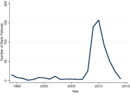
Figure 1. Number of bank failures over time.This figure plots the time series of bank fail-ures irrespective of resolution method—purchase and assumption (P&A) transaction, deposit payoff, or insured deposit transfer—during the period 1994 to 2013. Data are provided by the Federal Deposit Insurance Corporation and are available athttps://www.fdic.gov/bank/individual/ failed/banklist.html. The time series includes the failed banks whose resolution process was a P&A transaction or a deposit payoff but does not include open bank assistance. The time series document the spike in bank failures that occurred after 2008 following a relatively calm period between 1994 and 2007. (Color figure can be viewed at wileyonlinelibrary.com)
Following these arguments, in our empirical tests we proxy for the extent of misallocation by exploring which types of bidders are more likely to win auctions when other bidders are undercapitalized. More importantly, we show that, when potential acquirers in failed bank auctions have low capitalization, the FDIC’s revenues from selling failed banks are lower.
IV. Descriptive Statistics
Over the 2007 to 2013 sample period, a substantial number of banks were taken into receivership by the FDIC and then sold at auction. This fact can be seen clearly in Figure 1, which plots the number of bank failures from 1994 onward. From 1994 to 2006, the average number of bank failures per year was 5, and at no point exceeded 15. In contrast, 2010 witnessed a high of 157 bank failures.
Selling Failed Banks 1735
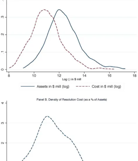
million and a standard deviation of $765 million. Figure 2, Panel B, shows that the resolution costs are sizable relative to the assets of a failed bank: the median resolution cost from 2007 to 2013 was 28% of the total assets of a failed bank.
Table I presents descriptive statistics for key variables used in our analy-sis for failed banks (Panel A), their acquirers (Panel B), and their potential acquirers, that is, banks that did not fail (Panel C) over the sample period. Failed banks tend to be smaller, experience higher losses on their loan portfo-lio, and have worse financial health relative to acquirers or potential acquirers. All banks tilt their lending to real estate, which comprises more than 60% of their asset portfolio. These patterns hold if we stratify the sample yearly rather than pooling the full sample. Relative to other banks, eventual acquirers tend to be larger and have a slightly larger residential and CRE tilt in their loan composition.
More interestingly, acquiring banks tend to be located closer to failed banks than other potential acquirers. The average distance between the eventual acquirer and a failed bank is 200 miles, as opposed to 900 miles for other potential acquirers. The loan portfolios of eventual acquirers are also more similar to those of the failed bank than are those of other potential acquirers. The average share of CRE loans for an eventual acquirer differs from that of the failed bank it acquired by 18 percentage points (pp), while for potential acquirers this difference is 35 pp. These patterns will be fundamental to the facts that we establish in our main analysis.
We also note some additional key statistics of failed banks and eventual acquirers in our sample. At the time of the failure, failed banks’ assets aver-age $759 million, with a standard deviation of $2.441 billion. These banks are largely state chartered (65%), and 5% are part of a bank holding company com-prising more than one commercial and savings bank. The assets of acquirers in the sample average $11.275 billion; 55% of acquirers are state chartered and 26% are organized as a multibank holding company.
In Table II, we present empirical results supporting some of these infer-ences. In particular, we estimate a logit of the event that a potential acquirer acquires a failed bank as a function of the financial and asset characteristics of the potential acquirer. Letting(.) denote a logit, we estimate the following specification:
Pryijt=1
=α+ŴiXit+ŴjXjt+µt+εijt
,
1736
The
Journal
of
Finance
R
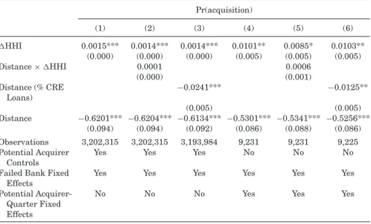
This table presents descriptive statistics for the main sample used in the analysis.Costis the cost borne by the FDIC in the resolution of each failed bank as a percentage of the total assets of the failed bank at the time of failure.P50 Tier 1 Capital Ratio of Local Potential Acquirersis the median Tier 1 capital ratio across the local potential acquirers of the failed bank. Local potential acquirers are potential acquirers whose branch network overlaps with that of the failed bank in at least one zip code. %Well-Capitalized Local Potential Acquirersis the percentage of local potential acquirers whose Tier 1 capital ratio is above the median Tier 1 capital ratio across local potential acquirers.P50 Tier 1 Capital Ratio ofHHI Potential Acquirers
is the median Tier 1 capital ratio of all potential acquirers whose acquisition of the failed bank would increase local deposit-based market concentration.
%Well-CapitalizedHHI Potential Acquirersis the percentage of potential acquirers whose Tier 1 capital ratio is above the median Tier 1 capital
ratio among the group of potential acquirers whose acquisition of the failed bank would increase local deposit-based market concentration.CODis the average coefficient of dispersion (COD) in sales ratio studies of property tax assessments of residential properties in the assessment jurisdictions where the failed bank operates branches.Publicly Tradedis an indicator variable that takes the value of one if the failed bank was registered with the SEC in the previous quarter.Sizeis defined as the total assets (RCFD2170) of the bank (in thousands).Liquidity Ratiois the ratio between liquid assets (cash+federal funds sold+securities (excluding MBS/ABS) and total assets. %Residential Loansis the percentage of residential loans relative to total loans (RCFD2122). %CRE Loansis the percentage of commercial and real estate (CRE) loans relative to total loans (RCFD2122). %C&I Loans
is the percentage of commercial and industrial (C&I) loans relative to total loans (RCFD2122). %Consumer Loansis the percentage of consumer loans relative to total loans (RCFD2122).30-89PD Ratiois the ratio of total loans that are 30-89 days past due (RCFD1406) to total loans.NPL Ratiois the ratio of nonperforming loans (nonaccrual) (RCFD1403) and 90 days or more past due (RCFD1407) to total loans.OREO Ratiois other real estate owned (RCFD2150) divided by total assets.Unused Commitment Ratiois unused commitments divided by unused commitments and total loans.Tier
1 Capital Ratiois the ratio between Tier 1 (core) capital and total risk-weighted assets.Leverage Ratiois the ratio between Tier 1 (core) capital and
(adjusted) total assets. %Core Depositsis total core deposits (transaction accounts+savings deposits+time deposits less than $100,000) divided by total deposits.Distanceis the average pairwise distance (in 100-mile increments) between all pairs of branches of the failed bank and potential acquirer.State Bankis an indicator variable that takes the value of one if the bank is regulated by a state regulator.Multibank BHCis an indicator variable that takes the value of one if the bank is part of a bank holding company that owns more that one commercial or savings bank.Distance
(%Res. Loans) is the absolute difference between the failed bank’s and the potential acquirer’s percentage of total loans held in residential loans.
Distance(%CRE Loans) is the absolute difference between the failed bank’s and the potential acquirer’s percentage of total loans held in CRE
loans.Distance(%CI Loans) is the absolute difference between the failed bank’s and the potential acquirer’s percentage of total loans held in C&I loans.Distance(%Cons. Loans) is the absolute difference between the failed bank’s and the potential acquirer’s percentage of total loans held in consumer loans.HHIis the average increase in local deposit market concentration that would result from potential acquirerjacquiring the branch network of failed banki.HHIranges from 0 to 1,000, where 0 indicates a merger that does not increase local market concentration and 1,000 indicates a merger that transforms a perfectly competitive local market into a local monopoly.
Panel A: Failed Banks
N Mean St. Dev. p25 p50 p75
Resolution Cost and Local Market Characteristics
Cost 438 0.281 0.120 0.200 0.273 0.366
Selling
Failed
B
anks
1737
Table I—Continued
Panel A: Failed Banks
N Mean St. Dev. p25 p50 p75
P50 Tier 1 Capital Ratio of Local Potential Acquirers 424 11.711 1.480 10.575 11.629 12.714 % Well-Capitalized Local Potential Acquirers 424 0.477 0.237 0.333 0.500 0.650 P50 Tier 1 Capital Ratio ofHHI Potential Acquirers 439 12.211 1.366 11.3 12.21 13.08 % Well-CapitalizedHHI Potential Acquirers 439 0.492 0.151 0.394 0.488 0.589
COD 317 13.546 7.477 9.600 11.500 15.640
Publicly Traded 434 0.260 0.439 0.000 0.000 1.000
Asset and Financial Characteristics
Size 438 759,751 2,441,545 102,913 210,851.5 492,491
Liquidity Ratio 438 16.288 7.666 10.621 15.041 20.605
% Residential Loans 438 26.250 19.312 12.311 23.314 32.692
% CRE Loans 438 57.481 19.805 46.353 60.259 70.157
% C&I Loans 438 10.777 8.909 4.544 8.455 14.439
% Consumer Loans 438 2.224 3.160 0.375 1.157 2.844
30-89PD Ratio 438 4.281 3.399 1.975 3.584 5.699
NPL Ratio 438 15.892 9.212 9.523 14.641 19.882
OREO Ratio 438 5.183 4.880 1.686 3.853 7.343
Unused Commitment Ratio 438 5.947 5.622 2.577 4.711 8.347
Tier 1 Capital Ratio 438 1.627 3.203 0.336 1.718 2.900
Leverage Ratio 438 1.231 2.219 0.276 1.260 2.110
% Core Deposits Ratio 438 72.056 14.046 63.208 74.108 81.522
State Bank 438 0.649 0.477 0 1 1
Multibank BHC 438 0.055 0.228 0 0 0
The
Journal
of
Finance
R
Table I—Continued
Panel B: Acquirers
N Mean St. Dev. p25 p50 p75
Asset Characteristics
Size 417 11,275,389 38,244,003 504,464 1,405,573 3,628,005
Liquidity Ratio 417 16.754 10.345 9.564 14.907 21.081
% Residential Loans 417 24.531 14.843 14.196 23.459 30.940
% CRE Loans 417 48.698 18.415 36.394 52.013 62.160
% C&I Loans 417 15.034 8.692 8.193 14.058 19.758
% Consumer Loans 417 5.212 7.148 0.969 2.627 7.165
30-89PD Ratio 417 1.323 1.183 0.524 0.968 1.731
NPL Ratio 417 3.924 4.962 1.123 2.301 4.557
OREO Ratio 417 0.964 1.264 0.166 0.522 1.201
Unused Commitment Ratio 417 14.320 8.327 8.866 13.683 18.373
Financial Characteristics
Tier 1 Capital Ratio 417 16.774 13.211 11.203 13.380 17.093
Leverage Ratio 417 10.695 5.179 8.260 9.690 11.730
% Core Deposits Ratio 417 80.512 9.145 74.877 81.990 86.855
State Bank 417 0.559 0.497 0 1 1
Multibank BHC 417 0.260 0.438 0 0 1
Proximity to Failed Bank
Distance 414 2.010 3.524 0.000 1.000 2.000
Distance (% Res. Loans) 416 15.293 14.672 4.691 10.841 21.110
Distance (% CRE Loans) 416 18.944 15.160 7.875 15.370 26.441
Distance (% C&I Loans) 416 8.916 7.723 3.078 7.104 11.992
Distance (% Cons. Loans) 416 4.530 6.630 0.784 1.977 5.999
HHI 417 31.277 148.884 0 0.021 0.947
Selling
Failed
B
anks
1739
Table I—Continued
Panel C: Potential Acquirers
N Mean St. Dev. p25 p50 p75
Asset Characteristics
Size 3,466,810 1,714,011 31,925,725 72,038 150,311 341,356
Liquidity Ratio 3,466,810 23.825 15.780 12.822 20.147 30.815
% Residential Loans 3,409,603 31.023 21.430 15.724 26.545 40.800
% CRE Loans 3,411,532 35.120 21.703 17.078 33.817 50.958
% C&I Loans 3,411,532 13.226 10.447 6.352 11.305 17.746
% Consumer Loans 3,411,532 6.671 10.016 1.437 3.914 8.197
30-89PD Ratio 3,411,532 1.441 1.640 0.348 0.956 1.971
NPL Ratio 3,411,470 2.629 3.812 0.490 1.486 3.287
OREO Ratio 3,457,074 0.745 1.473 0.000 0.216 0.843
Unused Commitment Ratio 3,404,039 10.628 7.726 5.415 9.899 14.820
Financial Characteristics
Tier 1 Capital Ratio 3,464,686 21.974 90.736 11.400 13.960 18.610
Leverage Ratio 3,464,693 11.587 10.588 8.300 9.540 11.660
% Core Deposits Ratio 3,431,750 79.639 11.717 74.227 81.467 87.250
State Bank 3,470,905 61.1 48.7 0 1 1
Proximity to Failed Bank
Distance 3,428,866 9.175 6.069 5.000 8.000 12.000
Distance (% Res. Loans) 3,401,228 22.085 19.260 7.546 16.560 30.807
Distance (% CRE Loans) 3,403,145 30.732 20.505 13.528 28.085 45.400
Distance (% C&I Loans) 3,403,145 10.127 9.582 3.482 7.563 13.786
Distance (% Cons. Loans) 3,403,145 6.041 9.663 1.207 3.242 7.251
Table II
Acquisition Likelihood and Potential Acquirer Characteristics
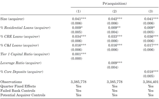
This table reports the coefficients from a logit regression. The dependent variable Pr(acquisition) takes the value of one if potential acquirer j acquires failed bank iand zero otherwise. Size (acquirer)is total assets (RCFD2170) measured using constant 2009:Q1 prices.% Residential Loans (acquirer)is the percentage of residential loans relative to total loans (RCFD2122).% CRE Loans
is the percentage of commercial and real estate (CRE) loans relative to total loans (RCFD2122).
% C&I Loansis the percentage of commercial and industrial (C&I) loans relative to total loans (RCFD2122).Tier 1 Capital Ratio (acquirer) is the ratio of Tier 1 (core) capital and total risk-weighted assets.Leverage ratio (acquirer)is the ratio of Tier 1 (core) capital and (adjusted) total assets.% Core Deposits (acquirer)is total core deposits (transaction accounts+savings deposits +time deposits less than $100,000) divided by total deposits. Other unreported control variables are:Liquidity Ratio, the ratio of liquid assets cash+federal funds sold+securities (excluding MBS/ABS) and total assets;Unused Commitment ratio, total unused commitments divided by the sum of total unused commitments and total loans;% Consumer Loans, the percentage of consumer loans relative to total loans (RCFD2122);NPL Ratio, the ratio of nonperforming loans (nonaccrual) (RCFD1403) and 90 days or more past due (RCFD1407) to total loans; andOREO Ratio, other real estate owned (RCFD2150) divided by total assets. Standard errors are presented in parentheses, and are clustered at the level of the failed bank’s state headquarters. ***, **, and * represent statistical significance at the 1%, 5%, and 10% levels, respectively.
Pr(acquisition)
(1) (2) (3)
Size (acquirer) 0.041*** 0.042*** 0.041***
(0.006) (0.006) (0.006)
%Residential Loans(acquirer) 0.009* 0.009** 0.009*
(0.005) (0.004) (0.005)
%CRE Loans(acquirer) 0.034*** 0.033*** 0.036***
(0.006) (0.006) (0.006)
%C&I Loans(acquirer) 0.016*** 0.016*** 0.017***
(0.006) (0.006) (0.006)
Tier 1 Capital Ratio(acquirer) 0.001*** (0.000)
Leverage Ratio(acquirer) 0.009*** (0.004)
%Core Deposits(acquirer) 0.018***
(0.005)
Observations 3,385,778 3,385,778 3,384,401
Quarter Fixed Effects Yes Yes Yes
Failed Bank Controls Yes Yes Yes
Potential Acquirer Controls Yes Yes Yes
acquirer’s characteristics in an economically meaningful way. For instance, a one-standard-deviation increase in the Tier 1 capital ratio of the potential acquirer increases the likelihood of acquisition by 7.6 pp, evaluated at the mean values of the other variables.8
8Similarly, the marginal effects of theLeverage Ratioand% Core Depositsvariables are also
Selling Failed Banks 1741
V. Willingness and Ability to Pay for a Failed Bank
In this section, we begin by documenting the characteristics of potential ac-quirers that drive the willingness to pay for a failed bank. In Section III, we show that potential acquirers whose willingness to pay is higher are more likely to win the auction. Conversely, if certain potential acquirers are more likely to acquire a given failed bank, we conclude that they value the bank more than other potential acquirers. Here, we explore three potential determinants of will-ingness to pay for a failed bank: geographic distance, asset specificity, and mar-ket concentration. Then, consistent with our framework, we examine whether potential acquirers’ capitalization impacts their ability to pay for a failed bank.
A. Willingness to Pay: The Role of Distance
A.1. Are Failed Banks Sold Nonlocally?
We begin our main analysis by asking whether the geographic proximity of a potential acquirer to a failed bank increases its willingness to pay for the failed bank. One could imagine that the proximity of the potential acquirer does not play a role. As Cochrane (2013) argues, failed banks could be “swiftly bought up by other banks even out of state.” If geographically proximate banks have a higher willingness to pay for a failed bank, they should be more likely to acquire it.
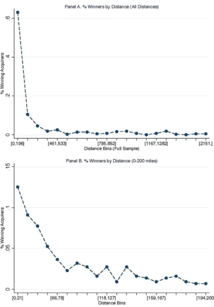
A simple cut of the raw data in Figure 3 suggests that failed banks are rarely sold to distant banks. In Figure3, Panel A, we sort potential acquirers into 20 bins, which contain an equal number of potential acquirers, by the average distance of their branch networks to that of the failed bank. More than 60% of failed banks during the sample period are acquired by the 5% of potential acquirers that are located closest to the failed bank. The distance of the branch networks of these potential acquirers from the branch network of the failed bank is less than 196 miles. The results are also striking if we restrict the sample to the 5% of potential acquirers closer to the failed bank, as in Figure 3, Panel B. The potential acquirers with an average branch network distance of less than 21 miles, which represent the 0.25% closest potential acquirers, acquire over 12% of failed banks. Similar patterns obtain when we use an alternative measure of distance in Appendix Figure A.1. These figures clearly show that most failed banks are sold very locally, and that the share of banks sold declines quickly with distance.
We formalize this insight by building on specification (1). Here, we estimate a conditional (fixed effect) logit specification: Letting (., µit) denote a fixed effect logit with aµitfixed effect, we estimate,9
Pryijt =1
=α+ŴXjt+β1dijt, µit
,
9The results presented in SectionVare robust to using a linear probability model instead of
Selling Failed Banks 1743
whereiindexes a failed bank being auctioned at timet, andjindexes a potential acquirer. The dependent variable, yi jt, is a dummy variable equal to one if potential bidder j acquired failed bank i at time t, and zero otherwise. The dependent variable of interest isdi jt, which measures the average distance of the branch network of the potential acquirer from the branch network of the failed bank. We control for characteristics of a potential acquirer, such as its asset size, loan composition, and capitalization, in Xjt.
In specification (2), we also condition on failed bank fixed effectsµit. We do so to ensure that our results are driven by the distance between the failed bank and the acquirer, not the characteristics of the bank being sold. One concern could be that failed banks that are geographically distant from potential ac-quirers also have worse assets, or assets that are very specific. Alternatively, state-level regulations or regulators may affect which types of banks are lo-cated in a given state (see Agarwal et al. (2014)), as well as the distance to potential acquirers. Failed bank fixed effectsµitcontrol for such possibilities. Moreover, failed bank fixed effects subsume any time variation such as aggre-gate trends in bank sales, since the failure happens at one point in time, as well as between-state variation. The variation in our estimates therefore comes from within-failed-bank differences in the geographic proximity of potential ac-quirers to the failed bank. We cluster standard errors at the level of the failed bank’s state headquarters.
Table III, Panel A, presents the results and confirms the intuition from Figure 3. The coefficient on distance, β1, is negative and statistically signif-icant. Potential acquirers that are located farther from a failed bank have a lower probability of acquiring it. This estimate is economically meaningful. The average marginal effect of a 100-mile increase in the distance between the failed bank’s and potential acquirer’s branch networks is to reduce the expected probability of acquisition by 3 pp. The effect of distance is stronger conditional on being located close to the failed bank: a 100-mile increase in distance re-duces the likelihood of acquisition by 13.6 pp for potential acquirers within 100 miles of the failed bank, but by only 0.25 pp for potential acquirers 1,000 miles away from the failed bank.
Next, we perform a series of robustness checks to further confirm that failed banks are sold very locally. To better understand the effect of distance, we restrict our subsample to acquirers whose branches are within a 200-mile radius. In unreported tests we find that the effect of distance persists when we restrict attention to the subsample of these more plausible potential acquirers. To ensure that our results are not driven by unobserved characteristics of potential acquirers, we include acquirer-quarter fixed effects,µjt, and estimate the following specification:10
Pryijt=1
=α+µjt+β1dijt, µit
.
10One potential concern with a fixed effects logit is the incidental parameters problem. The
The
Journal
of
Finance
R
Table III
Geographic Proximity and Failed Bank Acquisition Likelihood
This table reports the coefficients from a fixed effects logit regression. The dependent variable Pr(acquisition) takes the value of one if potential acquirerjacquires failed bankiand zero otherwise.Distanceis average pairwise distance (in 100-mile increments) between all pairs of branches of the failed bank and potential acquirer. Potential acquirer controls (unreported) includeSize, Liquidity Ratio, % CRE Loans, % C&I Loans, NPL Ratio,
OREO Ratio, Unused Commitment Ratio, andTier1 Capital Ratioas defined in TableI. Column (1) of Panel A includes failed bank fixed effects and
the above potential acquirer controls. The specifications in columns (2) and (3) of Panel A include potential acquirer and potential acquirer-quarter fixed effects, respectively. The introduction of potential acquirer and potential acquirer-quarter fixed effects eliminates observations with invariant dependent variables at the level of the potential acquirer and potential acquirer-quarter, resulting in a reduction in the number of observations from column (1) to columns (2) and (3). Panel B reports results from a fixed effects logit regression using the specification in column (3) of Panel A on coastal/noncoastal areas and on high/low house price growth areas (2001:Q1–2006:Q4).Coastalis an indicator variable taking the value of one if the headquarters of the failed bank is located in a coastal state, where coastal state is defined as any state with a coastline on the Atlantic Ocean, Pacific Ocean, and Great Lakes.High HPI growthis an indicator variable that takes the value of one if the house price index (HPI) growth in the failed bank’s branch service area over the 2001:Q1–2006:Q4 period is greater than the median HPI change for all failed banks. HPI growth is calculated using the all-transactions indexes at the metropolitan statistical area and state nonmetropolitan levels provided by the Federal Housing Finance Agency. We calculate the HPI growth for each failed bank by weighting the HPI growth variable for each bank by the percentage of deposits of the failed bank in each area. Panel C repeats the analysis of column (3) of Panel A after stratifying the sample based on above- and below-median level of CRE, residential, and C&I loans held across the failed banks in the sample. Standard errors are presented in parentheses, and are clustered at the level of the failed bank’s state headquarters. ***, **, and * represent statistical significance at the 1%, 5%, and 10% levels, respectively.
Panel A: Baseline Specification
Pr(acquisition)
(1) (2) (3)
Distance −0.624*** −0.679*** −0.545***
(0.095) (0.102) (0.089)
Observations 3,202,315 93,666 9,231
Failed Bank Fixed Effects Yes Yes Yes
Potential Acquirer Controls Yes Yes No
Potential Acquirer Fixed Effects No Yes No
Potential Acquirer-Quarter Fixed Effects No No Yes
Selling
Failed
B
anks
1745
Table III—Continued
Panel B: Heterogeneity Based on Failed Bank Regional Exposure
Pr(acquisition)
Coastal Noncoastal High HPI growth Low HPI growth
(1) (2) (3) (4)
Distance −0.420*** −0.712*** −0.375*** −0.865***
(0.087) (0.164) (0.056) (0.101)
Observations 4,819 4,412 4,644 4,587
Failed Bank Fixed Effects
Yes Yes Yes Yes
Potential Acquirer-Quarter Fixed Effects
Yes Yes Yes Yes
Panel C: Heterogeneity Based on Lending Specialization of Failed Banks
Pr(acquisition)
High CRE Low CRE High Residential Low Residential High C&I Low C&I
(1) (2) (3) (4) (5) (6)
Distance −0.466*** −0.636*** −0.565*** −0.526*** −0.575*** −0.510***
(0.090) (0.117) (0.118) (0.098) (0.123) (0.081)
Observations 4,607 4,624 4,652 4,579 4,735 4,496
Failed Bank Fixed Effects Yes Yes Yes Yes Yes Yes
All failed bank and acquirer factors are subsumed in the fixed effects. The remaining variation we exploit is the interaction between the characteristics of the potential acquirer and the failed bank and the relative distance between them. Because of the acquirer-quarter fixed effects, the sample of potential acquirers in these conditional logit tests is limited to banks that acquired a failed bank in the same quarter in which the failure occurred. In spite of this very limited sample, our results in columns (2) and (3) are quantitatively and qualitatively similar to the baseline estimates.
Because banks had substantial exposure to the real estate sector, we also explore how the house price dynamics that a failed bank faced shape the effect of distance (see Keys, Seru, and Vig (2012)). In TableIII, Panel B, we stratify the sample based on whether the failed bank is in a coastal area, which experienced larger boom-bust house price cycles during the last decade. We further stratify based on house price growth experienced in the failed bank region. The results presented in columns (1) to (4) show that, in each of these subsamples, distant banks have a lower probability of purchasing a failed bank. The estimated coefficients also suggest that the effect of distance is slightly less pronounced if failed banks are located in coastal states or operate in areas that experienced high house price growth between 2001 and 2006. For instance, a 100-mile increase in distance reduces the likelihood of acquisition by 2.6 and 3.1 pp in coastal and noncoastal states, respectively. Similarly, a 100-mile increase in distance reduces the likelihood of acquisition by 2.3 and 3.5 pp for failed banks located in areas with high and low house price growth, respectively. In TableIII, Panel C, we examine whether these effects vary based on failed banks’ specialization. We stratify failed banks based on the percentage of CRE, residential, and C&I loans held by the failed bank. The results in Table III, Panel C, show that the effects of distance are present across all subsamples, although sales are most local for failed banks with a low share of CRE loans.
Local potential acquirers may have a higher willingness to pay for a failed bank, resulting in local failed bank sales, for several reasons. A large literature shows that the transmission of soft information within banks declines with geo-graphic distance (Petersen and Rajan (2002), Stein (2002)). A distant potential acquirer will not be able to operate an acquired failed bank very efficiently because of the decrease in soft information. Nearby banks might also be bet-ter able to exploit economies of scale, such as lower overhead, easier servicing of branches and joint ATMs, or greater market power (Akkus, Cookson, and Hortacsu (2015)). Next, we explore the conjecture that the effect of distance in failed bank acquisitions is related to soft information loss.
A.2. Does Distance Reflect Soft Information?
Selling Failed Banks 1747
information contained in public tax assessments of real estate values, following Garmaise and Moskowitz (2004).11
Property tax authorities periodically evaluate the quality of property assess-ments in their jurisdictions. The most popular measure of assessment quality is the coefficient of dispersion (COD) used by Garmaise and Moskowitz (2004). The central input is the ratio between the market value of properties recently sold and their assessed value, which is frequently determined by statute. Sup-pose that the assessed value is legislated at 33% of market value. If assessments measure market values perfectly, then the ratios of assessed values to market value are the same for all assessed properties, 33%. Outside investors can then rely on the hard information collected by the tax authorities to closely track the market value of a property. If these ratios are dispersed, however, with, say, some assessed values at 10% of the actual value and others 50%, then assessed values provide little information to outside investors. The COD formally mea-sures how disperse are the ratios.12When public assessments are less accurate, this measure is larger and investors have to rely on soft information about local real estate market conditions rather than public assessments.
We exploit this measure to examine whether local banks are more likely to acquire a failed bank in areas with more soft information using the following specification:
Pryijt=1
=α+µjt+β1dijt+β2dijtCODij, µit
,
whereCODi jrepresents the COD, our measure of the importance of soft infor-mation in the real estate market. The level effect ofCODi jis absorbed by failed bank fixed effects,µit. Our independent variable of interest is the interaction between the distance of potential acquirers and the amount of soft informa-tion in the local market,di jCODi j. As in other specifications, we also include acquirer-quarter fixed effects, µjt, and cluster standard errors at the level of the failed bank’s state headquarters.
The results are presented in TableIV. In column (1), we use a dummy variable to capture the degree of soft information in a failed bank’s portfolio. Specifi-cally, we use an indicator that takes a value of one if the failed bank is in an above-median COD area (High COD) and zero otherwise. The coefficient on distance,β1, is negative and statistically significant, which indicates that dis-tant potential acquirers are less likely to acquire failed banks even in markets with less soft information. More importantly, as the interaction term reveals, local soft information significantly increases the advantage of local banks. If we compare areas with above-median soft information to those below median, we
11We follow Garmaise and Moskowitz (2004) and compute the measures based on
commer-cial real estate assessments. Banks also have substantial residential real estate holdings. For robustness, we recomputed the measure using residential real estate assessments and find similar results.
12The coefficient of dispersion is calculated asCOD= 1N
N i |Ri−Rmed|
Rmed ×100, where Ri is the assessment-to-market ratio for theithproperty sold, Rmedis the median assessment-to-market
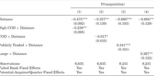
Table IV
Geographic Proximity and Failed Bank Acquisition: Interaction with Soft Information
This table reports results of a fixed effects logit regression. The dependent variable Pr(acquisition) takes the value of one if potential acquirerjacquires failed bankiand zero otherwise.Distance
is the average pairwise distance (in 100-mile increments) between all pairs of branches of the failed bank and potential acquirer.CODis the average coefficient of dispersion (COD) in sales ratio studies of property tax assessments of residential properties in the assessment jurisdictions where the failed bank operates branches.High CODis an indicator variable that takes the value one if COD is above the sample-median COD.Publicly Tradedis an indicator variable that takes the value of one if the failed bank was registered with the SEC in the previous quarter.Largeis an indicator variable that takes the value of one if the total assets of the failed bank are larger than the median size across failed banks in the quarter prior to failure. All specifications include failed bank fixed effects and potential acquirer-quarter fixed effects. Standard errors are presented in parentheses, and are clustered at the level of the failed bank’s state headquarters. ***, **, and * represent statistical significance at the 1%, 5%, and 10% levels, respectively.
Pr(acquisition)
(1) (2) (3) (4)
Distance −0.475*** −0.357** −0.668*** −0.694***
(0.092) (0.139) (0.103) (0.129)
High COD×Distance −0.238**
(0.095)
COD×Distance −0.017*
(0.010)
Publicly Traded×Distance 0.341***
(0.101)
Large×Distance 0.267**
(0.122)
Observations 6,635 6,635 9,231 9,231
Failed Bank Fixed Effects Yes Yes Yes Yes
Potential-Acquirer/Quarter Fixed Effects Yes Yes Yes Yes
find that the coefficient on distance increases over 50%. For potential acquirers within 100 miles of the failed bank, a 100-mile increase in distance reduces the likelihood of acquisition by 17.6 pp in high COD areas, whereas the same increase in low COD areas reduces the likelihood of acquisition by just 11.4 pp. The incremental effect of COD on the marginal effect of distance rapidly dis-appears as we move farther away from the failed bank. For potential acquirers within 300 miles from the failed bank, a 100-mile increase in distance reduces the likelihood of acquisition by 7.4 pp in high COD areas, whereas the same increase in low COD areas reduces the likelihood of acquisition by 6.5 pp. In column (2), we obtain similar inferences when we use a continuous measure of COD.
Garmaise and Moskowitz (2004) make a strong case that COD captures plau-sibly exogenous variation in soft information.13Even if that were not the case,
13They control for the level of heterogeneity in local properties and the house price growth rate
Selling Failed Banks 1749
the variation we use to identify our effect is based on the interaction between COD and the distance between a bank and a potential acquirer. Because we include both failed bank and acquirer-quarter fixed effects, these results are not driven by the fact that banks or potential acquirers are different in areas of high rather than low COD. To generate our results, areas with high admin-istrative mismeasurement would be areas in which local banks are arelatively better match for the failed bank in that area and a relatively worse match for distant failed banks on dimensions not related to distance or soft informa-tion. In areas with little administrative mismeasurement, the result would be reversed. We think this alternative, while possible, is unlikely.
We also use alternative measures of soft information. Following Granja (2013) and Agarwal et al. (2014), we measure whether the failed bank was publicly traded before failure and whether the failed bank is large relative to the sample of failed banks. The idea behind these proxies is that public infor-mation is more readily available for these banks. Soft and local inforinfor-mation should therefore play a larger role in acquiring private and smaller banks and in turn should provide an advantage to local potential acquirers. We confirm this conjecture in columns (3) and (4) of TableIV.
We also follow DeLong and DeYoung (2007) and investigate whether potential acquirers’ acquisition experience reduces frictions that arise with geographic distance. We hand-collect M&A data from the Merger description database available from the FRB Chicago. In Table Vwe find that potential acquirers who are active in the M&A market are also more likely to acquire a failed bank. Moreover, potential acquirers with a higher acquisition intensity pur-chase more geographically distant failed banks. These findings are consistent with the idea that acquisition strategy plays a role in failed bank allocation. In particular, potential acquirers that have greater M&A experience are more likely to be active in the failed banks market and are better able to overcome frictions that arise with distance.
Overall, the above results show that failed banks are generally acquired by very local banks and are rarely sold out of state. This effect is robust to failed bank and potential acquirer fixed effects, and is present across regions that saw different housing boom-bust cycles over the last decade as well as among failed banks with different specializations. These findings are more pronounced for banks in areas with more soft information. Taken together, these results suggest that the valuations of potential acquirers differ, with local banks having a higher willingness to pay for failed banks, especially in areas with pervasive soft information.
B. Willingness to Pay: The Role of Asset Specificity
Next, we examine whether asset specificity of failed banks affects poten-tial acquirers’ willingness to pay for them. Some failed banks focus more on
Table V
Geographic Proximity and Failed Bank Acquisition: Role of M&A Activity of Potential Acquirers
This table reports results of a fixed effects logit regression. The dependent variable Pr(acquisition) takes the value of one if potential acquirerjacquires failed bankiand zero otherwise.Distanceis the average pairwise distance (in 100-mile increments) between all pairs of branches of the failed bank and potential acquirer.M&A Nonfailed Bankis an indicator variable that takes the value of one if the potential acquirer acquired another bank through an unassisted M&A between 2007 and 2013.Number of M&A: Nonfailed Banksis the number of unassisted M&As that the potential acquirer completed between 2007 and 2013.Number of Failed Bank Acquisitionsis the number of failed bank acquisitions that the potential acquirer completed between 2007 and 2013. The first three specifications include failed bank fixed effects and potential acquirer controls. The last three specifications include failed bank fixed effects and potential acquirer-quarter fixed effects. Standard errors are presented in parentheses, and are clustered at the level of the failed bank’s state headquarters. ***, **, and * represent statistical significance at the 1%, 5%, and 10% levels, respectively.
Pr(acquisition)
(1) (2) (3) (4) (5) (6)
Distance −0.631*** −0.639*** −0.639*** −0.582*** −0.741*** −0.560*** (0.100) (0.095) (0.100) (0.104) (0.121) (0.090) M&A Nonfailed Bank 1.910***
(0.164) Number of M&A:
Nonfailed Banks
0.422*** (0.041) Number of Failed Bank
Acquisitions
0.651*** (0.057) Distance×M&A
Nonfailed Bank
0.084 (0.067) Distance×Number of
M&A: Nonfailed Banks
0.040*** (0.007)
Distance×Number of Failed Bank Acquisitions
0.018** (0.009)
Observations 3,201,353 3,201,353 3,201,452 9,231 9,231 9,231
Failed Bank Fixed Effects Yes Yes Yes Yes Yes Yes
Potential Acquirer Controls
Yes Yes Yes No No No
Potential
Acquirer-Quarter Fixed Effects
No No No Yes Yes Yes
Selling Failed Banks 1751
a higher willingness to pay for a failed bank, they should be more likely to acquire it.
There are substantial differences in the portfolio composition of failed banks. The average failed bank’s portfolio comprises 58% CRE loans, but there are large differences between failed banks, with a 20 pp standard deviation. For residential loans, the mean is 24% and standard deviation is 18 pp (TableI). As mentioned earlier, these substantial differences in portfolios are not unusual and are also observed among potential bidders and actual acquirers.
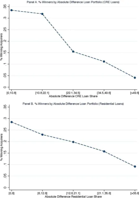
One simple way to examine whether failed banks are more likely to be ac-quired by banks with similar portfolios is to compute the correlation between the portfolios of the failed bank and the acquirer. The correlation between the share of CRE loans of acquirers and failed banks is 0.295, which indicates that failed banks are sold to acquirers with similar portfolios. This relationship can also be seen in Figure 4, Panel A, where we sort potential acquirers into quintiles based on their portfolio distance from the failed bank and then plot the share of failed banks (as a percentage of all failed banks in our sample) that were acquired by potential acquirers in different quintiles for the CRE portfolio distance measure. Approximately 33% of failed banks are acquired by the 20% of potential acquirers with the most similar share of CRE loans in their portfolio. Conversely, fewer than 5% of failed banks are acquired by the 20% of potential acquirers whose CRE portfolio shares are most dissimilar. A similar pattern obtains in Figure4, Panel B, where we sort potential acquirers by their residential loan portfolio share. These simple cuts of raw data suggest that failed banks are acquired by banks with similar portfolios. Results using other portfolio measures are similar, though substantially weaker. This is not surprising: most banks in our sample have their asset holdings in commercial and residential real estate.
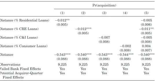
To formally examine whether similarity to the failed bank increases the probability of acquisition, we build on conditional logit specification from above and estimate:
Pryijt=1
=α+µjt+β1portfolio distanceijt+β2dijt, µit
,
whereyi jtis a dummy variable equal to one if potential bidderjacquired failed banki at timet, and zero otherwise. The independent variable of interest is
port f olio distancei jt, which measures the absolute difference in the loan