Can They be Alternatives to Variational Bayes?

Analysis of Empirical MAP and Empirical Partially Bayes:

Can They be Alternatives to Variational Bayes?

Shinichi Nakajima Masashi Sugiyama

Nikon Corporation Tokyo Institute of Technology

Abstract

Variational Bayesian (VB) learning is known to be a promising approximation to Bayesian learning with computational efficiency. How- ever, in some applications, e.g., large-scale collaborative filtering and tensor factoriza- tion, VB is still computationally too costly. In such cases, looser approximations such as MAP estimation and partially Bayesian (PB) learning, where a part of the parameters are point-estimated, seem attractive. In this pa- per, we theoretically investigate the behavior of the MAP and the PB solutions of matrix factorization. A notable finding is that the global solutions of MAP and PB in the em- pirical Bayesian scenario, where the hyperpa- rameters are also estimated from observation, are trivial and useless, while their local solu- tions behave similarly to the global solution of VB. This suggests that empirical MAP and empirical PB with local search can be alterna- tives to empirical VB equipped with the use- ful automatic relevance determination prop- erty. Experiments support our theory.

1 INTRODUCTION

In probabilistic models where Bayesian learning is computationally intractable, variational Bayesian (VB) approximation (Attias, 1999) is a promising al- ternative equipped with the useful automatic relevance determination (ARD) property (Neal, 1996). VB has experimentally shown its good performance in many applications (Bishop, 1999; Ghahramani and Beal, 2001; Jaakkola and Jordan, 2000; Barber and Chi- appa, 2006; Lim and Teh, 2007; Ilin and Raiko, 2010), Appearing in Proceedings of the 17^th International Con- ference on Artificial Intelligence and Statistics (AISTATS) 2014, Reykjavik, Iceland. JMLR: W&CP volume 33. Copy- right 2014 by the authors.

and its model selection accuracy has been theoretically guaranteed (Nakajima et al., 2012) in fully-observed Bayesian matrix factorization (MF) (Salakhutdinov and Mnih, 2008) or probabilistic PCA (Tipping and Bishop, 1999; Roweis and Ghahramani, 1999). Generally, VB is solved with efficient iterative local search algorithms. However, in some applications where even VB is computationally too costly, looser approximations, where all or a part of the parameters are point-estimated, with less computation costs are attractive alternatives. For example, Chu and Ghahra- mani (2009) applied partially Bayesian (PB) learning, where the core tensor is integrated out and the fac- tor matrices are point-estimated, to Tucker factoriza- tion (Kolda and Bader, 2009; Carroll and Chang, 1970; Harshman, 1970; Tucker, 1996). Mørup and Hansen (2009) applied the MAP estimation to Tucker factor- ization with the empirical Bayesian procedure, i.e., the hyperparameters are also estimated from observation. The empirical MAP estimation, with the same order of computation costs as the ordinary alternating least squares algorithm (Kolda and Bader, 2009), showed its model selection capability through the ARD property. On the other hand, it was shown that, in fully-observed MF, the objective function for empirical PB and em- pirical MAP is lower-unbounded at the origin, which implies that their global solutions are trivial and use- less (Nakajima and Sugiyama, 2011; Nakajima et al., 2011). Here, a question arises: Is there any essential difference between those factorization models? This paper answers to the question. We theoretically investigate the behavior of the local solutions of em- pirical PB and empirical MAP in fully-observed MF. More specifically, we obtain an analytic-form of the lo- cal solutions. A notable finding is that, although the global solutions of empirical PB and empirical MAP are useless, the local solutions behave similarly to the global solution of empirical VB. Experiments support our theory.

We also investigate empirical PB and empirical MAP in collaborative filtering (or partially observed MF)

and tensor factorization. We theoretically show that their global solutions are also trivial and useless, but experimentally show that, with local search, they work similarly to empirical VB.

2 BACKGROUND

In this section, we formulate the matrix factorization model, and introduce the free energy minimization framework, which contains VB, PB, and MAP.

2.1 Probabilistic Matrix Factorization

Assume that an observed matrix V _{∈ R}^L×M consists of the sum of a target matrix U _{∈ R}^L×M and a noise matrix_{E ∈ R}^L×M:

V = U +_E.

In matrix factorization (MF), the target matrix is as- sumed to be low rank, and can be factorized as

U = BA^⊤,

where A_{∈ R}^M×H, and B_{∈ R}^L×H. Thus, the rank of U is upper-bounded by H ≤ min(L, M).

In this paper, we consider the probabilistic MF model (Salakhutdinov and Mnih, 2008), where the observa- tion noiseE and the priors of A and B are assumed to be Gaussian:

p(V|A, B) ∝ exp⁽−2σ¹²∥V − BA^⊤∥²Fro

), (1) p(A)_{∝ exp}⁽₋¹₂tr⁽AC_A⁻¹A^⊤)), (2) p(B)_{∝ exp}⁽₋¹₂tr⁽BC_B⁻¹B^⊤)). (3) Here, we denote by ⊤ the transpose of a matrix or vector, by_{∥ · ∥}Frothe Frobenius norm, and by tr(_{·) the} trace of a matrix. We assume that the prior covariance matrices CAand CBare diagonal and positive definite, i.e.,

CA= diag(c²_a1, . . . , c²_aH), CB = diag(c²_b1, . . . , c²_bH) for cah, cbh > 0, h = 1, . . . , H. Without loss of general- ity, we assume that the diagonal entries of the product CACB are arranged in the non-increasing order, i.e., cahcbh _{≥ c}ah′^cbh′ for any pair h < h^′. Throughout the paper, we denote a column vector of a matrix by a bold small letter, and a row vector by a bold small letter with a tilde, namely,

A = (a1, . . . , aH) = (a_e1, . . . ,_ea_M)^⊤ _{∈ R}^M×H, B = (b1, . . . , bH) =⁽eb₁, . . . , eb_L^)⊤_{∈ R}^L×H.

2.2 Free Energy Minimization Framework for Approximate Bayesian Inference The Bayes posterior is given by

p(A, B_{|V ) =}^p(V |A,B)p(A)p(B)

p(V ) ^{, (4)}

where p(V ) = ⟨p(V |A, B)⟩p(A)p(B). Here, _⟨·⟩p de- notes the expectation over the distribution p. Since this expectation is hard to compute, many approxima- tion methods have been proposed, including sampling methods (Chen et al., 2001) and deterministic meth- ods (Attias, 1999; Minka, 2001). This paper focuses on deterministic approximation methods.

Let r(A, B), or r for short, be a trial distribution. The following functional with respect to r is called the free energy:

F (r) =^⟨log_p(V |A,B)p(A)p(B)^r(A,B)

⟩

r(A,B) ⁽⁵⁾

=^⟨log_{p(A,B|V )}^{r(A,B) ⟩}

r(A,B)− log p(V ). In the last equation, the first term is the Kullback- Leibler (KL) distance from the trial distribution to the Bayes posterior, and the second term is a constant. Therefore, minimizing the free energy (5) amounts to finding a distribution closest to the Bayes posterior in the sense of the KL distance. A general approach to approximate Bayesian inference is to find the mini- mizer of the free energy (5) with respect to r in some restricted function space. In the following subsections, we review three types of approximation methods with different restricted function spaces.

Let br be such a minimizer. We define the MF solution by the mean of the target matrix U :

U =b ^⟨BA^⊤⟩_br(A,B). (6) The hyperparameters (CA, CB) can also be estimated by minimizing the free energy:

( bCA, bCB) = argmin_CA,CB(minrF (r; CA, CB)) . This approach is referred to as the empirical Bayesian procedure, on which this paper focuses.

Let

V =^{∑min(L,M )}_h=1 γh^ωbh^ω⊤_ah (7) be the singular value decomposition (SVD) of V . In the three approximate Bayesian methods discussed in this paper, the MF solution can be written as trun- cated shrinkage SVD, i.e,

U =b

∑H h=1

bγh^ωbh^ω

⊤ah, where bγh=

{γ˘h if γh≥ γ_h^, 0 otherwise. ⁽⁸⁾ Here, γ_his a truncation threshold and ˘γhis a shrinkage estimator, respectively, both of which depend on the approximation method.

2.3 Empirical Variational Bayes

In the VB approximation, the independence between the entangled parameter matrices A and B is assumed: r^VB(A, B) = r_A^VB(A)r_B^VB(B). (9) Under this constraint, a tractable local search al- gorithm for minimizing the free energy (5) was de- rived (Bishop, 1999; Lim and Teh, 2007). Further- more, Nakajima et al. (2012) have recently derived an analytic-form of the global solution when the observed matrix V has no missing entry:

Proposition 1 (Nakajima et al., 2012) Let K = min(L, M ), K = max(L, M ), α = K/K. Let κ = κ(α) (> 1) be the zero-cross point of the fol- lowing decreasing function:

Ξ (κ; α) = Φ (^√ακ) + Φ^(√κ_α⁾, where Φ(x) = ^log(x+1)_{x −}¹₂.

Then, the empirical VB solution is given by Eq.(8) with the following truncation threshold and shrinkage estimator:

γ^EVB

h ^{= σ}

√

M + L +^√LM⁽κ +_κ¹⁾, (10)

˘

γ_h^EVB=^γ₂^h (

1₋^{(M +L)σ}_γ2 ²

h ⁺

√(1₋^{(M +L)σ}_γ2 ² h

)2

−^{4LM σ}γ_h^{4 4}

) . (11) 2.4 Empirical Partially Bayes

Point-estimation amounts to approximating the distri- bution with the delta function. PB-A learning point- estimates B, while PB-B learning point-estimates A, respectively, i.e.,

r^PB-A(A, B) = r^PB-A_A (A)δ(B; bB), (12) r^PB-B(A, B) = δ(A; bA)r_B^PB-B(B), (13) where δ(B; bB) denotes the (pseudo-)Dirac delta func- tion of B located at B = bB.¹ PB learning chooses the one, giving a lower free energy, of the PB-A and the PB-B solutions (Nakajima et al., 2011).

Analyzing the free energy, Nakajima et al. (2011) showed that the global solution of empirical PB is use- less:

1By the pseudo-Dirac delta function, we mean an extremely localized density function, e.g., δ(B; bB) ∝ exp⁽−^{∥B− b}_2ε^B∥2Fro) with a very small but strictly positive variance ε > 0, such that its tail effect can be neglected, while its negative entropy χB = ⟨log δ(B; bB)⟩_{δ(B; bB)} re- mains finite.

Proposition 2 (Nakajima et al., 2011) The empirical PB solution is bγh^EPB= 0, regardless of observation. 2.5 Empirical MAP

In the maximum a posteriori (MAP) estimation, all the parameters are point-estimated, i.e.,

r^MAP(A, B) = δ(A; bA)δ(B; bB). (14) The global solution of empirical MAP is also useless: Proposition 3 (Nakajima and Sugiyama, 2011) The empirical MAP solution is bγh^EMAP = 0, regardless of observation.

3 THEORETICAL ANALYSIS

As explained in Section 2, previous theoretical work proved that the global solutions of empirical PB and empirical MAP are trivial in fully-observed MF. In this section, we however show that empirical PB and empirical MAP have non-trivial local solutions, which behave like the global solution of empirical VB. 3.1 Analytic-forms of Non-trivial Local

Solutions

Due to the diagonality, proven by Nakajima et al. (2013), of the VB posterior covariances, the VB pos- terior can be expressed as

r(A, B)_∝^∏H_h=1exp (

−^∥ah2σ^−b2_ah^ah∥2 −^∥bh2σ^−b2bh∥2

bh

) , (15)

with a_bh = ah^ωah, and bb_h = bh^ωbh. Then, the free energy (5) can be explicitly written as follows:

F = ₂¹⁽LM log(2πσ²) +^{∥V ∥}_σ2^Fro2 +^∑H_h=12Fh

) , (16) where

2Fh= M log ^c

2 ah

σ²_ah ^{+ L log} c²_bh σ²_bh ⁺

a²h^{+M σ} 2 ah

c²_ah ⁺ b²h^+Lσ

2 bh

c²_bh

− (L + M) +^{−2ahbhγh+(a}

2 h^{+M σ}

2

ah)(^b2h^+Lσ 2 bh)

σ^{2 . (17)}

The free energy of PB and MAP can also be expressed by Eq.(16) with some factors in Eq.(17) smashed: σ²_bh → ε for a very small constant ε > 0 in PB-A and MAP, and σ²_ah → ε in PB-B and MAP. Below, we neglect the large constants related to the entropy, i.e.,_{−L log σb}²_h in PB-A and MAP, and_{−M log σa}²_h in PB-B and MAP. We fix the ratio between the hyper- parameters to cah/cbh = 1, since the ratio does not affect the estimation of the other parameters.

We can give an intuition of Proposition 2 and Propo- sition 3, i.e., why the global solutions of empirical PB and empirical MAP are useless. Consider the empirical PB-A solution, which minimizes the PB-A free energy:

2F_h^PB-A= M log ^c

2 ah

σ²_ah ^{+ L log c} 2 bh⁺

a²h^{+M σ} 2 ah

c²_ah ⁺ b²_h c²_bh

+^{−2ahbhγh+(a}

2

h+M σ_ah² ₎b²h

σ^{2 + const. (18)}

Clearly, Eq.(18) diverges to _{−∞ as c}ahcbh _{→ 0 with}

ah= bh= 0, σ²_ah = cahcbh, and therefore,

(bcahbcbh)^EPB-A _{→ 0} (19) is the global solution. The same applies to empirical PB-B and empirical MAP, which leads to the useless trivial estimators, i.e.,

bγ^EPBh = bγh^{EMAP= 0. (20)}

Note that this phenomenon is caused by smashing a part of the posterior, which makes the infinitely large entropy constant: In empirical VB without smashing, the first four terms in Eq.(17) balance the prior and the posterior variances, and Eq.(17) is lower-bounded.² Nevertheless, we will show that empirical PB and em- pirical MAP with local search can work similarly to empirical VB. We obtain the following theorems: Theorem 1 The PB free energy has a non-trivial lo- cal minimum such that

ahbh= ˘γ_h^local-EPB if and only if γh> γ^local-EPB

h ^{, (21)}

where γ^local-EPB

h ^{= σ}

√

L + M +^√2LM + K², (22)

˘

γ_h^local-EPB= ^γ₂^h (

1 + ^−Kσ

2₊^√

γ_h⁴−2(L+M)σ²γ_h²+K²σ⁴ γ_h²

) . (23) (Sketch of proof) The PB-A solution given c²_ah and c²_bh has been obtained by Nakajima et al. (2011). Substi- tuting it into the free energy (18), we can write the PB-A free energy as a function of cahcbh. By taking the first derivative, we obtain the stationary points. By checking the sign of the second derivative, we pick up the non-trivial local minimum from those station- ary points. We can analyze the PB-B free energy in

2Hyperprior on c²a_h and c²b_h can make the free energy in PB and MAP lower-bounded. However, for the purpose of ARD, it should be almost non-informative. With such an almost non-informative hyperprior, e.g., the inverge- Gamma, p(c²a_h, c²b_h) ∝ (c²a_hc²b_h)^1.001+ 0.001/(c²a_hc²b_h), used in Bishop (1999), a deep valley exists close to the origin, which makes the global estimator uselessly conservative.

0 0.2 0.4 0.6

−0.1

−0.05 0

cahcbh

Fh/(LM)

VB PB MAP

(a) γh= 10

0 0.2 0.4 0.6

−0.1

−0.05 0

cahcbh

Fh/(LM)

VB PB MAP

(b) γh= 12

0 0.2 0.4 0.6

−0.1

−0.05 0

cah^cbh

Fh/(LM)

VB PB MAP

(c) γh= 14

0 0.2 0.4 0.6

−0.1

−0.05 0

cah^cbh

Fh/(LM)

VB PB MAP

(d) γh= 16

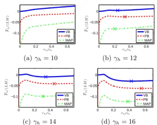
Figure 1: Free Energy dependence on cahcbh, where L = 20, M = 50. A cross indicates a non-trivial local minimum.

the same way, and obtain its local minimum. Choosing the one of PB-A and PB-B giving a lower free energy leads to the solution (21), which completes the proof.

✷

Theorem 2 The free energy of empirical MAP has a non-trivial local minimum such that

ahbh= ˘γ_h^local-MAP if and only if γh> γ^local-MAP_h , (24) where

γ^local-EMAP

h ^{= σ}

√2(M + L), (25)

˘

γ_h^local-EMAP=¹ 2

(

γh+^√γ_h²_{− 2σ}²(M + L) )

. (26)

(Sketch of proof) Similarly to the proof of Theorem 1, we substitute the MAP solution (Srebro et al., 2005; Nakajima and Sugiyama, 2011) given c²_ah and c²_bh into the MAP free energy or the negative log likelihood:

2F_h^MAP= M log c²_ah+ L log c²_bh+_c^a2^2h ah ⁺

b²h

c²_bh

+^−2ahbh_σ^γ2^h+a2hb2h + const. (27) By taking the first derivative, we find that the sta- tionary condition is written as a quadratic function of cahcbh. Analyzing the stationary condition, we obtain the local minimum (24), which completes the proof. ✷ Figure 1 shows the free energy as a function of cahcbh

(minimized with respect to the other parameters), i.e., Fh(cahcbh) = min

(ah,bh,σ²_ah,σ²_bh)^{Fh. (28)}

This exhibits the behavior of local minima of empiri- cal VB, empirical PB, and empirical MAP. We see that the free energy around the trivial solution cahcbh _{→ 0}

is different, but the behavior of a non-trivial local min- imum is similar: it appears when the observed singular value γhexceeds a threshold.

The boundedness is essential when we stick to the global solution. The VB free energy is lower-bounded at the origin, which enables inference consistently based on the minimum free energy principle. However, as long as we rely on local search, the unboundedness at the origin is not essential in practice. Assume that a non-trivial local minimum exists, and we perform local search only once. Then, whether local search for empirical PB (empirical MAP) converges to the trivial global solution or the non-trivial local solution simply depends on the initialization. Note that this also applies to empirical VB, where local search is not guaranteed to converge to the global solution, because of the multi-modality of the free energy.

3.2 Behavior of Local Solutions

Let us define, for each singular component, a local em- pirical PB (local empirical MAP) estimator to be the estimator equal to the non-trivial local minimum if it exists, and the trivial global minimum otherwise. The analytic-form of the non-trivial local minimum is given by Theorem 1 (Theorem 2). We suppose that local search for empirical PB (empirical MAP) looks for this solution.

In the rest of this section, we investigate the local em- pirical PB and the local empirical MAP estimators with their analytic-forms. We will also experimentally investigate the behavior of local search algorithms in Section 5.

Let us consider the normalized singular values of the observation and the estimators:

γ_h^′ = √^γh

Kσ^{2, bγ} h′ ^{= b}

γh

√Kσ^{2, γ}

′ h⁼

γ_h

√Kσ^{2, ˘γ} h′ ⁼

˘ γh

√Kσ^2.

Then, the estimators can be written as functions of α = K/K:

γ^′EVB_h = σ

√

1 + α +^√α⁽κ +_κ¹⁾, (29)

˘

γ^′EVB_h =^γ₂^h′ (

1₋^(1+α)σ_γ′2 ²

h ⁺

√(1₋^(1+α)σ_γ′2 ² h

)2

−^4ασ_γh^′44 )

, (30)

γ^′local-EPB

h ^{= σ}

√

1 + α +^√2α + α², (31)

˘

γ^′local-EPB_h =^γ₂^h′ (

1 + ^−σ

2+^√γ_h^′4_−2(1+α)σ²γ^′2_h+σ⁴ γh^′2

) , (32) γ′local-EMAP

h ^{= σ}

√2(1 + α), (33)

˘

γ′local-EMAP

h ⁼

1 2

( γ_h^′ +

√

γ^′2_{h − 2σ}²(1 + α) )

. (34)

0 0.5 1 1.5 2

0 0.5 1 1.5 2

γ^′h bγ′h

EVB l o c al - EPB l o c a- EM AP

(a) Empirical Bayes.

0 0.5 1 1.5 2

0 0.5 1 1.5 2

γ^′h bγ′h

VB PBM AP

(b) Non-empirical Bayes with ca_h = cb_h = 100.

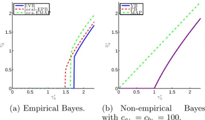
Figure 2: Behavior of empirical and non-empirical Bayesian estimators for α = K/K = 1/3.

0 0.2 0.4 0.6 0.8 1

0 0.5 1 1.5 2 2.5

α γ′ h

EVB l o c al - EPB l o c al - EM AP M PUL

Figure 3: Truncation thresholds. Note that κ is also a function of α.

The left graph in Figure 2 compares the behavior of the empirical VB, the local empirical PB, and the local empirical MAP estimators. We see the similarity be- tween those three empirical Bayesian estimators. This is in contrast to the non-empirical Bayesian estimators, where the hyperparameters CA, CB are given (see the right graph in Figure 2). There, VB and PB behave similarly, but MAP behaves like the maximum likeli- hood estimator (Nakajima et al., 2011).

Figure 3 compares the truncation thresholds (29), (31), and (33) of the estimators. We find that the thresh- olds behave similarly. However, an essential difference of local empirical PB from empirical VB and local em- pirical MAP is found: It holds that, for any α,

γ^′local-EPB< γ^′MPUL _{≤ γ}^′EVB, γ′local-EMAP_{, (35)}

where γ^′MPUL = (1 +^√α)

is the Marˇcenko-Pastur upper limit (MPUL) (Marˇcenko and Pastur, 1967; Nakajima et al., 2012), which is also shown in Figure 3. MPUL is the largest singular value of an L × M random matrix when the matrix consists of zero-mean independent noise, and its size L and M goes to infinity with fixed α. Inequalities (35) imply that, with high probability, empirical VB and local empirical MAP discard the singular components dominated by noise, while local empirical PB overestimates the rank when the ratio ξ = H^∗/K between the (unknown) true rank and the possible largest rank is small, i.e., when most of the

singular components consist of noise.

4 PRACTICAL APPLICATIONS

In fully-observed MF, the analytic solution of VB (Proposition 1) is available, and therefore, one takes no advantage by substituting PB or MAP for VB. However, in other models, e.g., collaborative filter- ing (or partially-observed MF) and tensor factoriza- tion, no analytic-form solution has been derived, and all the state-of-the-art algorithms are local search. In such cases, approximating VB by PB or MAP reduces the memory consumption and calculation time, be- cause inverse calculations for estimating posterior co- variances can be skipped. In this section, we show that, also in collaborative filtering and tensor factor- ization, the global solutions of empirical PB and em- pirical MAP are trivial and useless. In Section 5, we will experimentally show that local search algorithms however tend to find useful local minima. We also mention the possibility of noise variance estimation. 4.1 Collaborative Filtering

In the collaborative filtering (CF) setting, the observed matrix V has missing entries, and the likelihood (1) is replaced with

p(V_{|A, B)∝exp}⁽_−2σ¹2_∥PΛ(V )_{− P}Λ(BA^⊤)_∥²_Fro⁾, (36) where Λ denotes the set of observed indices, and

(_PΛ(V ))_l,m=

{Vl,m if (l, m)_{∈ Λ,} 0 otherwise.

An iterative local search algorithm for empirical VB has been derived (Lim and Teh, 2007), similarly to the fully-observed case.

We can show that the global solutions for empirical PB and empirical MAP are useless also in this case: Lemma 1 All elements of the global empirical PB and the global empirical MAP solutions in CF are zero, regardless of observation.

Nevertheless, we experimentally show in Section 5 that local search for empirical PB and empirical MAP be- haves like local search for empirical VB.

4.2 Tensor Factorization

By extending MF to N -mode tensor data, the Bayesian Tucker factorization (TF) model was pro- posed (Chu and Ghahramani, 2009; Mørup and Hansen, 2009):

p(_Y|G,{A⁽ⁿ⁾_})∝exp (

− ∥^Y−G×1A

(1)···×^{NA(N )}_∥² 2σ²

) , (37)

p(_G)∝exp (

−^{vec(G)⊤(CG(N )⊗···⊗CG(1))}

−1vec(G) 2

) , (38)

p(_{A⁽ⁿ⁾_{}) ∝ exp} (

−

∑N

n=1^tr(A(n)C_A(n)^{−1 A(n)⊤)}

2

)

, (39)

where _{Y ∈ R}^∏Nn=1M(n), _{G ∈ R}^∏Nn=1H(n), and _{A⁽ⁿ⁾_∈ R^M(n)×H(n)} are an observed tensor, a core tensor, and factor matrices, respectively. Here, _×n, _{⊗, and} vec(·) denote the n-mode tensor product, the Kro- necker product, and the vectorization operator, re- spectively (Kolda and Bader, 2009). _{CG⁽ⁿ⁾_{} and} {CA⁽ⁿ⁾} are the prior covariances restricted to be di- agonal. We fix the ratio between the prior covari- ances to C_G⁽ⁿ⁾C_A⁻¹(n) = I_H⁽ⁿ⁾, where Id denotes the d-dimensional identity matrix.

Chu and Ghahramani (2009) applied non-empirical PB learning, where the core tensor is integrated out, and the factor matrices are point-estimated. Their model corresponds to Eqs.(37)–(39) with C_G⁽ⁿ⁾ = C_A⁽ⁿ⁾= I_H⁽ⁿ⁾. Mørup and Hansen (2009) applied em- pirical MAP to this model, and experimentally showed its model selection ability through the ARD property. However, we can show that the global solutions of em- pirical PB and empirical MAP are useless also in TF: Lemma 2 All elements of the global empirical PB and the global empirical MAP solutions in TF are zero, regardless of observation.

Nevertheless, our experiments in Section 5, as well as the experiments in Mørup and Hansen (2009), show that empirical PB and empirical MAP with local search are useful alternatives to empirical VB.

4.3 Noise Variance Estimation

Generally, the noise variance, σ² in Eq.(1), can be estimated based on free energy minimization. Naka- jima et al. (2012) obtained a sufficient condition for the perfect rank recovery by empirical VB with the noise variance estimated. However, we experimentally found that, when the noise variance is estimated, lo- cal search for empirical PB tends to underestimate the noise variance. Even worse, local search for empirical MAP tends to result in b^σ2→ 0.

This unreliability was pointed out by Mørup and Hansen (2009) in empirical MAP for TF. They sug- gested to set the noise variance under the assumption that the signal to noise ratio (SNR) is 0 db, i.e., the signal and the noise have equal energy. In this paper, we follow their approach in the experiments with real datasets, where the noise variance is unknown, and leave further investigation as future work.

0 500 1000 1500 2000 2500 2.02

2.04 2.06 2.08 2.1 2.12 2.14

Iteration

F/(LM)

EVB(Analytic) EVB(Iterative)

(a) Free energy

0 500 1000 1500 2000 2500

0 20 40 60 80 100

Iteration b H

EVB(Analytic) EVB(Iterative)

(b) Estimated rank

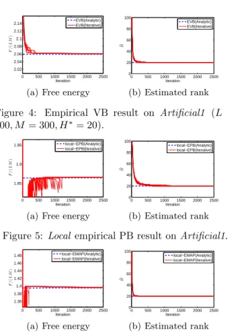
Figure 4: Empirical VB result on Artificial1 (L = 100, M = 300, H^∗= 20).

0 500 1000 1500 2000 2500

1.85 1.9 1.95

Iteration

F/(LM)

local−EPB(Analytic) local−EPB(Iterative)

(a) Free energy

0 500 1000 1500 2000 2500

0 20 40 60 80 100

Iteration b H

local−EPB(Analytic) local−EPB(Iterative)

(b) Estimated rank

Figure 5: Local empirical PB result on Artificial1.

0 500 1000 1500 2000 2500

1.36 1.38 1.4 1.42 1.44 1.46 1.48

Iteration

F/(LM)

local−EMAP(Analytic) local−EMAP(Iterative)

(a) Free energy

0 500 1000 1500 2000 2500

0 20 40 60 80 100

Iteration b H

local−EMAP(Analytic) local−EMAP(Iterative)

(b) Estimated rank

Figure 6: Local empirical MAP result on Artificial1.

5 EXPERIMENT

In this section, we experimentally show that empirical PB and empirical MAP with local search can be alter- natives to empirical VB. We start from fully-observed MF, where we can see how often local search finds the analytic local empirical solution. After that, we con- duct experiments in CF and TF.

For local search, efficient algorithms can be imple- mented based on the gradient descent algorithm (Chu and Ghahramani, 2009; Mørup and Hansen, 2009). However, it requires pruning, and we found that the pruning strategy can significantly affect the result, es- pecially in the estimated rank. Accordingly, we used the iterated conditional modes (ICM) algorithm (Be- sag, 1986; Bishop, 2006) without pruning, which we found is more stable, for all empirical Bayesian meth- ods. In all experiments, the entries of the mean parameters, e.g., bA, bB, and bG, were initialized with independent draws from _N1(0, 1), while the covari- ance parameters were initialized to the identity, e.g., ΣA= ΣB = CA= CB= IH.

5.1 Fully-observed MF

We first conducted an experiment with an artificial (Artificial1 ) dataset, following Nakajima et al. (2013).

0 500 1000 1500 2000 2500

0 5 10 15 20

Iteration b H

EVB local−EPB local−EMAP

(a) ArtificialCF.

0 500 1000 1500 2000 2500

0 5 10 15 20

Iteration b H

EVB local−EPB local−EMAP

(b) MovieLens.

Figure 7: Estimated rank in collaborative filtering with 99% missing ratio.

We randomly created true matrices A^∗_{∈ R}^M×H∗ and B^∗ _{∈ R}^L×H∗ so that each entry of A^∗ and B^∗ follows N¹(0, 1). An observed matrix V was created by adding a noise subject to _N1(0, 1) to each entry of B^∗A^∗⊤. Figures 4–6 show the free energy and the estimated rank over iterations for the Artificial1 dataset with the data matrix size L = 100 and M = 300, and the true rank H^∗ = 20. The noise variance was assumed to be known, σ² = 1. We performed iterative local search 10 times, starting from different initial points, and each trial is plotted by a solid line in the figures. We see that iterative local search tends to successfully find the analytic local empirical solution, although it is not the global solution.

We also conducted experiments on another artificial dataset and benchmark datasets. The results are sum- marized in Table 1. Artificial2 was created in the same way as Artificial1 with L = 400, M = 500, and H^∗= 5. The benchmark datasets were collected from the UCI repository (Asuncion and Newman, 2007). We set the noise variance under the assumption that the SNR is 0 db, following Mørup and Hansen (2009). In the table, the estimated ranks by the analytic- form solution and the ones by iterative local search are shown. The percentages for iterative local search indicate the frequencies over 10 trials. We can ob- serve the following: First, iterative local search tends to consistently estimate the same rank as the analytic solution over the trials.³ Second, the estimated rank tends to be consistent over empirical VB, local em- pirical PB, and local empirical MAP, and the correct rank is found on the artificial datasets. Exceptions are Artificial2, where local empirical PB overestimates the rank, and Optical Digits and Satellite, where local em- pirical MAP estimates a smaller rank than the others. These phenomena can be explained by the theoreti- cal implications in Section 3.2: In Artificial2, the ratio ξ = H^∗/K = 5/400 between the true rank and the pos-

3The results of empirical VB are different from the ones reported in Nakajima et al. (2013), where the noise vari- ance is also estimated from observation. Generally, the 0 db SNR assumption (Mørup and Hansen, 2009) tends to result in a smaller rank than empirical VB with noise vari- ance estimation (Nakajima et al., 2013) in our experiments.

Table 1: Estimated rank in fully-observed MF experiments.

Data set M L H^∗ Hb^EVB Hb^local-EPB Hb^local-EMAP

Analytic Iterative Analytic Iterative Analytic Iterative

Artificial1 300 100 20 20 20 (100%) 20 20 (100%) 20 20 (100%)

Artificial2 500 400 5 5 5 (100%) 8 8 (90%) 5 5 (100%)

9 (10%)

Chart 600 60 – 2 2 (100%) 2 2 (100%) 2 2 (100%)

Glass 214 9 – 1 1 (100%) 1 1 (100%) 1 1 (100%)

Optical Digits 5620 64 – 10 10 (100%) 10 10 (100%) 6 6 (100%)

Satellite 6435 36 – 2 2 (100%) 2 2 (100%) 1 1 (100%)

Table 2: Estimated rank (effective size of core tensor) in TF experiments.

Data set M H^∗ Hb^EVB Hb^local-EPB Hb^local-EMAP Hb^ARD-Tucker ArtificialTF (30, 40, 50) (3, 4, 5) (3, 4, 5): 100% (3, 4, 5): 100% (3, 4, 5): 90% (3, 4, 4): 80%

(3, 7, 5): 10% (3, 4, 5): 20% FIA (12, 100, 89) (3, 6, 4) (3, 5, 3): 100% (3, 5, 3): 100% (3, 5, 2): 50% (3, 2, 2): 40% (4, 5, 2): 20% (2, 1, 2): 20% (5, 4, 2): 10% (2, 3, 2): 10% (4, 4, 2): 10% (2, 2, 2): 10% (8, 5, 2): 10% (1, 1, 1): 10% (10, 4, 3): 10%

sible largest rank is small, which means that most of the singular components consist of noise. In this case, local empirical PB with its lower truncation threshold than MPUL fails to discard noise components (see Fig- ure 3). In Optical Digits and Satellite, α(= 64/5620 for Optical Digits and = 36/6435 for Satellite) is ex- tremely small, and therefore local empirical MAP with its higher truncation threshold tends to discard more components than the others, as Figure 3 implies.

5.2 Collaborative Filtering

To investigate the behavior of the estimators in CF, we conducted experiments with an artificial (Artifi- cialCF ) and the MovieLens datasets.⁴ The Artifi- cialCF dataset was created in the same way as the fully-observed case for L = 2000, M = 5000, and H^∗= 5, and masked 99% of the entries as missing values. For the MovieLens dataset (with L = 943, M = 1682), we randomly selected observed values so that 99% of the entries are missing.

Figure 7 shows the estimated rank over iterations. We see that all three methods tend to estimate the same rank, but empirical PB tends to give a larger rank, as in the fully-observed case.

5.3 Tensor Factorization

Finally, we conducted experiments on TF. We created an artificial (ArtificialTF ) dataset, following Mørup and Hansen (2009): We drew a 3-mode random tensor of the size of (M⁽¹⁾, M⁽²⁾, M⁽³⁾) = (30, 40, 50) with the signal components with (H^(1)∗, H^(2)∗, H^(3)∗) = (3, 4, 5). The noise is added so that the SNR is 0 db.

4http://www.grouplens.org/

As a benchmark, we used the Flow Injection Analy- sis (FIA) dataset.⁵ Table 2 shows the estimated rank with frequencies over 10 trials. Here, we also show the result by ARD Tucker with the ridge prior (Mørup and Hansen, 2009), of which the objective function is exactly the same as our empirical MAP. A slight dif- ference comes from the iterative algorithm (ICM vs. gradient descent) and the initialization strategy. We generally observe that the three empirical Bayesian methods provide reasonable results, although local em- pirical MAP is less stable than the others.

6 CONCLUSION

In this paper, we analyzed partially Bayesian (PB) learning and MAP estimation under the empirical Bayesian scenario, where the hyperparameters are also estimated from observation. Our theoretical analysis in fully-observed matrix factorization (MF) revealed a notable fact: Although the global solutions of empiri- cal PB and empirical MAP are trivial and useless, their local solutions behave similarly to the global solution of variational Bayesian (VB) learning.

We also conducted experiments in collaborative fil- tering (or partially observed MF) and tensor factor- ization, and showed that empirical PB and empirical MAP solved by local search can be good alternatives to empirical VB.

Acknowledgments

The authors thank reviewers for helpful comments. SN and MS thank the support from MEXT Kakenhi 23120004 and the CREST program, respectively.

5http://www.models.kvl.dk/datasets

References

A. Asuncion and D.J. Newman. UCI machine learn- ing repository, 2007. URL http://www.ics.uci.edu/

~mlearn/MLRepository.html.

H. Attias. Inferring parameters and structure of latent variable models by variational Bayes. In Proc. of UAI, pages 21–30, 1999.

D. Barber and S. Chiappa. Unified inference for varia- tional Bayesian linear Gaussian state-space models. In Advances in NIPS, volume 19, 2006.

J. Besag. On the statistical analysis of dirty pictures. Jour- nal of the Royal Statistical Society B, 48:259–302, 1986. C. M. Bishop. Variational principal components. In Proc. of International Conference on Artificial Neural Net- works, volume 1, pages 514–509, 1999.

C. M. Bishop. Pattern Recognition and Machine Learning. Springer, New York, NY, USA, 2006.

J. D. Carroll and J. J. Chang. Analysis of individual dif- ferences in multidimensional scaling via an N-way gen- eralization of ’Eckart-Young’ decomposition. Psychome- trika, 35:283–319, 1970.

M. H. Chen, Q. M. Shao, and J. G. Ibrahim. Monte Carlo Methods for Bayesian Computation. Springer, 2001. W. Chu and Z. Ghahramani. Probabilistic models for in-

complete multi-dimensional arrays. In Proceedings of International Conference on Artificial Intelligence and Statistics, 2009.

Z. Ghahramani and M. J. Beal. Graphical models and variational methods. In Advanced Mean Field Methods, pages 161–177. MIT Press, 2001.

R. A. Harshman. Foundations of the parafac procedure: Models and conditions for an ”explanatory” multimodal factor analysis. UCLA Working Papers in Phonetics, 16: 1–84, 1970.

A. Ilin and T. Raiko. Practical approaches to principal component analysis in the presence of missing values. Journal of Machine Learning Research, 11:1957–2000, 2010.

T. S. Jaakkola and M. I. Jordan. Bayesian parameter esti- mation via variational methods. Statistics and Comput- ing, 10:25–37, 2000.

T. G. Kolda and B. W. Bader. Tensor decompositions and applications. SIAM Review, 51(3):455–500, 2009. Y. J. Lim and Y. W. Teh. Variational Bayesian approach

to movie rating prediction. In Proceedings of KDD Cup and Workshop, 2007.

V. A. Marˇcenko and L. A. Pastur. Distribution of eigen- values for some sets of random matrices. Mathematics of the USSR-Sbornik, 1(4):457–483, 1967.

T. P. Minka. Expectation propagation for approximate Bayesian inference. In Proc. of UAI, pages 362–369, 2001.

M. Mørup and L. R. Hansen. Automatic relevance determi- nation for multi-way models. Journal of Chemometrics, 23:352–363, 2009.

S. Nakajima and M. Sugiyama. Theoretical analysis of Bayesian matrix factorization. Journal of Machine Learning Research, 12:2579–2644, 2011.

S. Nakajima, M. Sugiyama, and S. D. Babacan. On Bayesian PCA: Automatic dimensionality selection and analytic solution. In Proceedings of 28th International Conference on Machine Learning (ICML2011), pages 497–504, Bellevue, WA, USA, Jun. 28–Jul.2 2011. S. Nakajima, R. Tomioka, M. Sugiyama, and S. D. Baba-

can. Perfect dimensionality recovery by variational Bayesian PCA. In P. Bartlett, F. C. N. Pereira, C. J. C. Burges, L. Bottou, and K. Q. Weinberger, editors, Ad- vances in Neural Information Processing Systems 25, pages 980–988, 2012.

S. Nakajima, M. Sugiyama, S. D. Babacan, and R. Tomioka. Global analytic solution of fully-observed variational Bayesian matrix factorization. Journal of Machine Learning Research, 14:1–37, 2013.

R. M. Neal. Bayesian Learning for Neural Networks. Springer, 1996.

S. Roweis and Z. Ghahramani. A unifying review of lin- ear Gaussian models. Neural Computation, 11:305–345, 1999.

R. Salakhutdinov and A. Mnih. Probabilistic matrix fac- torization. In J. C. Platt, D. Koller, Y. Singer, and S. Roweis, editors, Advances in Neural Information Pro- cessing Systems 20, pages 1257–1264, Cambridge, MA, 2008. MIT Press.

N. Srebro, J. Rennie, and T. Jaakkola. Maximum margin matrix factorization. In Advances in Neural Information Processing Systems 17, 2005.

M. E. Tipping and C. M. Bishop. Probabilistic principal component analysis. Journal of the Royal Statistical So- ciety, 61:611–622, 1999.

L. R. Tucker. Some mathematical notes on three-mode factor analysis. Psychometrika, 31:279–311, 1996.

APPENDIX—SUPPLEMENTARY MATERIAL

A Proof of Theorem 1

We start from the PB solution given c²_ah and c²_bh, derived by Nakajima et al. (2011). Proposition 4 (Nakajima et al., 2011) The PB-MF posterior is given by

r^PB(A, B) =







r^PB-A(A, B) if L < M, r^PB-A(A, B) or r^PB-B(A, B) if L = M, r^PB-B(A, B) if L > M,

(40)

where r^PB-A(A, B) and r^PB-B(A, B) are the PB-A posterior and the PB-B posterior, respectively. The PB-A posterior is given by

r^PB-A(A, B) =

∏H h=1

N^M(ah;ab^PB-Ah ^{, σ}a^{2 PB-A}h ^IM)δ(bh; bb^PB-A_h ), (41)

where

b a^PB-A_h =

√

bγ_h^PB-AbδPB-A_h ^ωah, (42)

bb^PB-A_h =

√

bγh^PB-A/bδ PB-A

h ^{ωbh, (43)}

σ_a^{2 PB-A}_h = ^σ

2

bγh^PB-A/bδ PB-A

h ^{+ σ}

2

c²_ah

, (44)

bδ^PB-A_h = c²_ah

( M +

√

M²+ 4_c2^γ2h ah^c2bh

)

2γh

, (45)

and bγh^PB-A is the PB-A solution written as Eq.(8) with the following truncation threshold and the shrinkage estimator:

γ^PB-A

h ^{= σ}

√

M + ^σ

2

c²_ahc²_bh^{, (46)}

˘ γ_h^PB-A=





1 − σ²

( M +

√

M²+ 4_c2^γh2 ah^c2bh

)

2γ_h²





 γ^{h. (47)}

The PB-B posterior is given by

r^PB-B(A, B) = δ(ah;a_b^PB-B_h )

∏H h=1

N^{L(bh; bbPB-B}h ^{, σ2 PB-B}bh ^IL), (48)

where

b a^PB-B_h =

√ bγh^PB-Bbδ

PB-B

h ^{ωah, (49)}

bb^PB-B_h =

√

bγh^PB-B/bδ PB-B

h ^{ωbh, (50)}

σ_b^{2 PB-B}_h = ^σ

2

bγh^PB-Bbδ PB-B

h ^{+ σ}

2

c²_bh

, (51)

(bδ^PB-B_h )⁻¹= c²_bh

( L +

√

L²+ 4_c2^γh2 ah^c2bh

)

2γh

, (52)

and bγh^PB-B is the PB-B solution written as Eq.(8) with the following truncation threshold and the shrinkage estimator:

γ^PB-B

h ^{= σ}

√

L + ^σ

2

c²_ahc²_bh^{, (53)}

bγh^PB-B=





1 − σ²

( L +

√

L²+ 4_c2^γh2 ah^c2bh

)

2γ_h²





 γ^{h. (54)}

We first find the local solutions for empirical PB-A. For PB-A, the free energy (16) is written as

2F_h^PB−A= M log ^c

2ah

σ_a²_h ^{+ L log c}

2 bh⁺

a²_h+ M σ_a²_h c²_ah ⁺

b²_h c²_bh ⁺

−2a^hbhγh+(a2h^{+ M σ}a²h

)b²_h

σ^{2 − M +}

χB

H ^{. (55)} We neglect the last two terms in Eq.(55), which are (huge but) constant.

Substituting Eqs.(42)–(44) into Eq.(55), we have

2F_h^PB−A=_{−L log s}h+ M log⁽ch_bγh^PB-A/bδ^′PB-A_h + σ²⁾+ L log ch

+^bγ

PB-A

h ^bδh^′PB-A+ bγh^PB-A/bδh^′PB-A

ch

+^−2bγ

PB-A

h ^γh+ (bγh^PB-A)2

σ^{2 + const., (56)}

which is a function of

ch_{≡ c}ahcbh, sh≡ cah/cbh. Here, we used

δb_h^′PB-A= s⁻¹_h bδ^PB-A_h .

Although Eq.(56) goes to _{−∞ as s}h → ∞, we can fix the ratio sh for arbitrary value without any effect on determination of the product ch. We set sh= 1.

Since we look for non-trivial local minima of the free energy (56), we focus on the case when bγh^{PB-A > 0.}

Substituting Eqs.(47) and (45) into Eq.(56), we have

2F_h^PB−A= M log (

−M +

√

M²+ 4^γ

2 h

c²_h )

+^{2M + L} 2 ^{log c}

2 h⁺

√

M²+ 4^γ

2 h

c²_h ⁻ σ²

c²_h ^{+ const.. (57)}

Here, we used the following

bγ^PB-Ah ^/bδ′PB-Ah ⁼

ch

(

−^{(M +2σ}c²_h²

) +

√

M²+ 4^γ_c^2h

h

)

2 ^,

δb_h^′PB-A+ (bδ^′PB-A_h )⁻¹ = ch

√

M²+ 4^γ_c^h2² h

γh

.

The derivative of Eq.(57) with respect to c²_h is given by

2^∂F

PB−A h

∂c²_h ⁼⁻

4M γ_h² 2c⁴_ahc⁴_bh

(

−M +

√

M²+ 4^γ_c^h2² h

) √

M²+ 4^γ_c^h2² h

+^{2M + L} 2c²_h ⁻

4γ_h² 2c⁴_h

√

M²+ 4^γ_c2^h2 h

+^σ

2

c⁴_h