最近の更新履歴 Takashi SHIMIZU

Exit and Voice in a Marriage Market

Akiko Maruyama, Takashi Shimizu^y, and Kazuhiro Yamamoto^z March 2, 2009

Abstract

In this paper, we present a model in which agents choose voice, exit, or stay options when their marital condition becomes bad. The “voice” option can be interpreted as a spouse’s e¤ort or “investment” in the household to resolve his/her dissatisfaction and improve the marital condition. If a spouse hopes to divorce, he/she chooses the “exit” option. If a spouse does not hope to express his/her opinion and divorce, he/she chooses the “stay” option. We focus on the role of “exit” and “voice” in a marriage and investigate the e¤ects of a divorce law that is based on fault or no-fault on divorce rates. Our study shows that divorce rates tend to be too high under a unilateral divorce law in the non-transferable utility case. On the other hand, mutual-consent divorce law generates multiple equilibria, and divorce rates are then ine¢cient even in the transferable utility case. In this multiple equilibrium case, divorce rates are determined by social factors, such as culture, norm, and religion.

JEL classi…cation: D1; K0; R2

Key words: Divorce; Exit; Voice; Divorce law

National Graduate Institute for Policy Studies (GRIPS), 7-22-1 Roppongi, Minato-ku, Tokyo 106-8677, Japan. E-mail: [email protected].

yFaculty of Economics, Kansai University, 3-3-35 Yamate-cho, Suita, Osaka 564-8680, Japan. E-mail: [email protected].

zGraduate School of Economics, Osaka University, 1-7, Machikaneyama, Toyonaka, Osaka, Japan. E-mail: [email protected]

1 Introduction

In their seminal paper, Becker (1993) and Becker, Landes, and Michael (1977) insist that the Coase theorem applies to marital bargaining. To be more precise, a change in divorce law does not a¤ect the divorce rate if bargaining can be done without costs within a marriage. However, in the real world, the divorce law matters. In most of the U.S., the transition from “fault” to

“no-fault” divorce law occurred in the 1970s, and, simultaneously, the U.S. divorce rate rose dramatically. Whether these two trends are linked or not has been throughly investrgated. ¹ In recent years, empirical studies have shown that the change to no-fault unilateral divorce laws caused an increase in the divorce rate in U.S.. However, this e¤ect did not continue for long. For instance, Wolfer (2006) shows that the divorce rate is largely a¤ected in the …rst few years and is not a¤ected in the following years by the transition to unilateral divorce laws. On the other hand, a recent theoretical analysis shows that the change of the divorce law a¤ects the divorce rate. For example, Rasul (2005) shows that the change to unilateral divorce law reduced the marriage rate through a rise in the divorce rate. Clark (1999) and Fella, Mariotti, and Manzini (2004) show that an ine¢cient divorce may occur even under fault mutual-consent divorce law. Moreover, Chiappori, Iyigun, and Weiss (2007) show that a change in divorce laws can increase or decrease the divorce rate. Their research commonly shows that studying the e¤ects of divorce laws on divorce rates and welfare is still important.

In this paper, we investigate the e¤ect of divorce laws on the divorce rates and welfare with the “exit-voice framework” initiated by Hirschman (1970). Hirschman reports that “voice” and

“exit” are alternative means of dealing with problems that arise within an ongoing relationship or organization. “Voice” is an option to state dissatisfaction, negotiate with the partners, and try to restore the condition of the organization. If most members cooperate, the “voice” option can improve the condition of the organization. On the other hand, the “exit” is an option to depart from the organization itself.

A married couple is an organization in which a wife and a husband are partners. In the Palgrave Dictionary of Economics, Hirschman (1987) reports that “[m]odern marriage is one of the simplest illustrations of an exit-voice alternative. When a marriage is in di¢culty, the partners can either make an attempt, usually through a great deal of voicing, to reconstruct their relationship, or they can divorce.” In this paper, we formalize an exit-voice framework of the marriage market. To do so, we employ a simpli…ed version of Mortensen and Pissarides’ (1994) labor search model as our basic model.

In the research by Mortensen and Pissarides (1994), workers search for a job, and …rms search for workers. When they are matched, they form a production unit. However, there is a possibility that job condition switch from good to bad. Following their setting, we assume that both the female and the male search for a marriage partner in a marriage market. Each agent is randomly matched with another one, with whom he/she marries. A marriage always

1For example, Peters (1986) shows that the change to no-fault unilateral divorce does not a¤ect the divorce rate in her empirical work. On the other hand, Allen (1992) reports that the change to no-fault divorce causes a rise in the divorce rate. Then, Peter (1992) challenged the position presented by Allen (1992) in his paper. Friedberg (1998) suggests that the adoption of unilateral divorce laws has caused an increase in the divorce rate since the late 1960s.

starts in a good state (happy marriage). However, a marriage in a good state changes to bad (unhappy marriage) with constant positive probability per time. Therefore, in our model, there are three states of any agent: single, in a marriage in a good state, and in a marriage in a bad state. When spouses are in an unhappy marriage, each one chooses among the three options: voice, exit, or stay. Exit means a divorce. On the other hand, we regard voice as an option in which both a wife and a husband cooperate to restore a bad marital condition. To be more precise, voice is an e¤ort or “(post-marital) investment” within the household, and it costs. For example, a spouse can express his/her opinions to another in a costly manner in order to resolve his/her dissatisfaction. These opinions may be requests or claims for housework, expressions of a¤ection, the disciplining of children, and money matters. If both spouses express their voice, they may lead to a quarrel or an argument. A quarrel is, more or less, costly, although it may serve to improve the marital condition. If a spouse does not hope to divorce or to express his/her opinion, stay is an option.

We consider two cases: transferable utility and non-transferable utility. In the case of trans- ferable utility, all possible costs are transferable. Then, the voice cost is equal among spouses. On the other hand, in the case of non-transferable utility, the voice cost may be asymmetry among spouses. We focus on the case of non-transferable utility in this paper, since it is gener- ally assumed that utility is non-transferable in a couple (see, Zelder (1993), Fella, Manzini, and Mariotti (2007)). Analysis of the transferable utility case is relegated to Appendix C.

The main …ndings are as follows. The change in divorce law in‡uences the divorce rates and welfare. First, let us assume that divorce law is unilateral, i.e., a husband (wife) can divorce without the wife’s (husband’s) agreement. If the voice cost is higher for the husband (wife) than for the wife (husband), then a husband (wife) may reject the voice although the voice maximizes the sum of the spouse’s payo¤. Therefore, the voice under a unilateral divorce is often ine¢cient relative to the optimal case. In this case, equilibrium divorce rates are higher than optimal divorce rates. Thus, our results indicate that divorce rates tend to be too high under unilateral divorce law. Under unilateral divorce law, the factor that brings the economy about ine¢cient divorce is an asymmetry of the voice cost between a husband and a wife.²

Second, let us assume that divorce law is a mutual-consent law. Under the mutual-consent law, multiple equilibria may occur. In other words, an ine¢cient divorce or an ine¢cient voice may occur according to the social norms, culture, or religion. Under mutual-consent divorce law, both the voice and divorce (exit) options need the agreements of both a husband and a wife for realization. If both agents do not agree with each other, the couple continues to stay in a bad marital condition, which lowers the utility of both agents. Then, if both agents agree with one of two options, neither agent has an incentive to explore other options. In this multiple equilibrium case, divorce rates are determined by social factors such as culture, norm, and religion. In a society in which divorce is a bad behavior from an ethical viewpoint, agents in a bad marital condition may hesitate to choose a divorce option and choose a voice option instead. In such a society, divorce rates tend to be low when there are multiple equilibria. However, when there are multiple equilibria, there may be too many couples who select a voice option: divorce rates

2If the divorce cost is symmetric in couples, the equilibrium under unilateral divorce law is consistent with optimal case. See Appendix C.

are too low relative to the optimal condition, while asymmetry of voice cost induces too many divorces. If the economy is in this condition, the change in divorce law from mutual-consent to unilateral improves the welfare of the economy.³

The organization of this paper is as follows. In Section 2, we present a basic set-up of the model. In Section 3, we analyze the stationary distributions at equilibrium and compare their welfare levels. In Section 4, we show the situation in which a marital sate becomes bad. In Section 5, we study the non-transferable utility case and analyze the e¤ect of a unilateral divorce law and mutual-consent divorce law on divorce rates and welfare of the economy. Section 6 is the conclusion.

2 The Model

2.1 Environment

Time is continuous. There are a continuum of males (M) with measure 1 and one of females (F) with measure 1. Each agent is at one of three states: single, in a marriage in a good state (state g), and in a marriage in a bad state (state b). At the single stage, both the male and the female get a ‡ow payo¤ 0 and search for their marriage partners in a marriage market. On the equilibrium path, each agent randomly meets another agent on the other side with a Poisson rate a per time and marries him/her. When a marriage occurs, both agents enter into the marriage in a good state. In a marriage in a good state, both agents get the ‡ow payo¤ yg. However, a marriage in a good state becomes a marriage in a bad state with the Poisson process with _g per time. In a marriage in a bad state, both agents receive the ‡ow payo¤ yb, where yg ^{> y}b ^>0. A marriage in a bad state ends up in a divorce with the Poisson process with b. When a marriage ends up in a divorce, both the female and the male become single and search for a partner in the marriage market again. Every agent maximizes his/her lifetime expected discounted utility with the discount rate r.

Here, we de…ne that u is the measure of a single M or F, and e_j is the measure of marriages in state j. Thus, it must hold that u + eg+ eb= 1.

In our model, we assume that agents in a marriage in a bad state can make an e¤ort to restore the condition of the marriage. We call this e¤ort “voice.” We think that voice is a form of communication, such as that which occurs during a quarrel between a husband and wife. When a marital condition turns bad, a couple chooses a voice, a stay, or an exit option (divorce).

3The transferable utility case is an important benchmark, in which it is con…rmed that the Coase theorem holds and that the optimal options are chosen at the equilibrium if a husband and a wife coordinate on a Pareto- superior action pro…le. The equilibrium is consistent with optimal case under unilateral divorce law when the utility is transferable. However, when a husband and a wife cannot coordinate, multiple equilibria occur under a mutual-consent divorce law. Then, in the transferable utility case without coordination, the change in divorce law in‡uences the divorce rates and welfare.

Therefore, the ine¢cient results are always caused by mutual-consent divorce law if a couple cannot coordinate on a Pareto superior action pro…le. In both the transferable and the non-transferable utility case, mutual-consent divorce law always generates multiple equilibria, and then the divorce rate and the voice are ine¢cient. This comes from the fact that not only “voice” but also “exit” need the agreements of both a husband and a wife under mutual-consent divorce law.

Choosing a voice option, it costs vi = iv for i = M; F , and a bad condition becomes good with a Poisson rate per time, where _M + _F = 1 and = _M > ¹₂.⁴ Voice is e¤ective only when both partners choose it.

In addition, we assume that utility is non-transferable in the main text. The analysis of a transferable utility case is in the Appendix C.

2.2 Stationary Equilibria and Divorce Laws

In this environment, we restrict our attention to the class of stationary equilibria. The candidates for stationary equilibrium are as follows:

Voice equilibrium; the voice option is exercised in every marriage in a bad marital state. Exit equilibrium; the exit option is exercised in every marriage in a bad marital state. Stay equilibrium; the stay option is exercised in every marriage in a bad marital state. Generally, the option that is e¤ective depends not only on a spouse’s action but also on which divorce law is applied. In this paper, we consider the following divorce laws:

Unilateral divorce law. Mutual-consent divorce law.

The unilateral divorce law is one in which a husband (wife) can divorce without the agreement of his wife (her husband). On the other hand, under a mutual-consent divorce law, a mutual agreement is necessary before divorce.

In this paper, we analyze the e¤ects of divorce law on the condition under which the three types of equilibrium are reached and the welfare at the equilibrium.

3 Stationary Distribution and Welfare

In this paper, we restrict our attention to the steady state. In this section, we derive stationary distributions at equilibrium and compare their measures of the agents in each state, divorce rates, and welfare levels. In a steady state, the measure of agents in each state, denoted by u, eg and e_b, becomes constant throughout time.

First, the stationary conditions of the voice equilibrium are u^Va+ e^V_b = e^V_{g g}; e^V_{g g} = e^V_b( b+ );

4When we assume that F >¹₂, the results in our model are sustained.

where upperscript V represents that the variables are at the voice equilibrium. Since u^V + e^V_g + e^V_b = 1, we obtain

u^V = ^{g b}

a( g+ b+ ) + g b

; e^V_g = ^{a( b+ )}

a( _g+ _b+ ) + _{g b}^;

e^V_b = ^{a g}

a( g+ b+ ) + g b

: Second, the stationary conditions of the exit equilibrium are

u^Ea= e^E_{u g}; 0 = e^E_{b b}: Then, we obtain

u^E = ^g a+ g

; e^E_g = ^a

a+ g

; e^E_b = 0:

Third, the stationary conditions of the stay equilibrium are u^Sa= e^S_g g;

e^S_{g g} = e^S_{b b}: Then, we obtain

u^S = ^{g b}

a( g+ b) + g b

; e^S_g = ^{a b}

a( g+ _b) + g b

; e^S_b = ^{a g}

a( g+ b) + g b

:

Now, we are in a position to compare these stationary equilibria. First, the comparison of measures of the agents in single, state g, and state b among stationary states is as follows:

u^E > u^S > u^V;

(e^E_g > e^V_g > e^S_g; if a > ; e^V_g > e^E_g > e^S_g; if a < ; e^S_b > e^V_b > e^E_b :

We can also de…ne the divorce rate ^j in j equilibrium as follows:

V ₌ b^eV_b ^; E ₌

g^eE_g^; S₌

be^S_b: Then, we obtain

E _> S _> V_:

This result is fairly intuitive. In an exit equilibrium, a couple chooses to divorce as soon as they consider their marital condition bad. Therefore, the divorce rate, under such circumstances, is the highest. On the other hand, in a voice equilibrium, a couple tries to restore its marital condition, which results in a reduction in the divorce rate, since divorce does not occur in good marriages. Thus, the divorce rate is the lowest in a voice equilibrium.

Next, we derive the welfare at each equilibrium. The welfare is de…ned as the average value. In the voice and stay equilibria, there are three type of agents, single, marriage in a good state, marriage in a bad state. On the other hand, in an exit equilibrium, there are no agents for marriages in a bad state. This is because, in this equilibrium, agents select to divorce when the marriage state switches from good to bad.

Welfare in each equilibrium is

W^V = 2yge^V_v + (2y_b v)e^V_b ; W^E = 2yge^E_g;

W^S = 2y_ge^S_g + 2y_be^S_b: Then, the comparison of each equilibrium is as follows:

[w ^VE] W^V 8

< :

>

=

< 9

=

;

W^E , ¹ 2^v

8

< :

<

=

> 9

=

; a

g+ a^{yg+ yb;}

[w ^ES] W^E 8

< :

>

=

< 9

=

;

W^S , yb

8

< :

<

=

> 9

=

; a

g+ a^yg;

[w ^SV] W^S 8

< :

>

=

< 9

=

;

W^V , ¹ 2^v

8

< :

>

=

< 9

=

;

f(a + b)yg ^aybg a( g+ _b) + g b

:

The optimal option is illustrated in Figures 1 and 2. Note that Line w-VE is upward and Line w-SV is downward.⁵ We distinguish two cases: a > and a < .

5Throughout this paper, we adopt a convention, i.e., the cuto¤ line of a condition, such as [w-VE], is called Line w-VE.

4 A Couple’s Game in Bad Marital State

The situation that a couple faces when its marital state becomes bad is a kind of game played by both spouses. Before investigating the stationary equilibrium at full length, we clarify the equilibrium conditions of the couple’s game in a bad marital state under each divorce law.

The point is that spouses may need to coordinate in order to exercise one option. The voice option always needs to be coordinated. The exit option needs to be coordinated only under the mutual-consent divorce law. This brings about di¤erent equilibrium conditions between two divorce laws.

In the present paper, we use iteratively (weakly) undominated equilibrium as an equilibrium concept. Iteratively undominated equilibrium is a Nash equilibrium that survives against an iter- ative elimination of weakly dominated strategies. Generally, a result of the iterative elimination of weakly dominated strategies is dependent upon the order of eliminations, and, therefore, an iteratively undominated equilibrium is often thought to be problematic. However, it is veri…ed that, in the games we consider in the present paper, the order of iteration does not matter. For example, Marx and Swinkels (1997) show that an order of iteration does not matter in the class of games satisfying a “TDI condition.” It is veri…ed that any version of the couple’s game in the present paper satis…es the TDI condition.

Let ^j_i be i’s payo¤ when j option is exercised by the couple. These payo¤s are endogenously derived in later analysis. Throughout this section, we use the following two assumptions: Assumption 1 For each i = M; F , ^V_i , ^E_i , and ^S_i are all distinct.

Assumption 2

V

M ^EM ^VF ^EF^; V

M ^SM ^VF ^SF^; E

M ^SM ^{= E}F ^SF^:

These assumptions hold in a later analysis of the matching model. Assumption 1 is made to circumvent a complicated characterization of equilibria. Since we employ an iteratively undom- inated equilibrium, the equilibrium conditions are quite complicated when any two distinctive strategies give the same payo¤. Assumption 2 refers to the situation in which the di¤erence between the payo¤s received in the voice option and other options of M is lower than F, and the di¤erence between the payo¤s received in the exit option and the stay option is common for M and F. This assumption is relevant for the later analysis because we assume there is no di¤erence between M and F except for the instantaneous voice cost and M’s instantaneous voice cost is larger than F’s.

4.1 Unilateral Divorce Law

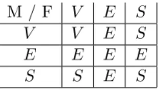
We …rst consider the unilateral divorce law. The couple’s game in a bad marital state is illustrated by the matrix in Table 1. Each entry is an e¤ective option for the couple.

M / F V E S

V V E S

E E E E

S S E S

Table 1: The game under the unilateral divorce law

Proposition 1 Let us assume that Assumptions 1 and 2 hold. Then, the equilibrium conditions for each type of equilibria under the unilateral divorce law are as follows:

1. Voice equilibrium: ^V_M > ^E_M and ^V_M > ^S_M. 2. Exit equilibrium: ^E_M > ^V_M and ^E_M > ^S_M. 3. Stay equilibrium: ^S_M > ^V_M and ^S_M > ^E_M.

The formal proof is relegated to Appendix A. A parameter set satisfying the equilibrium conditions for one type of equilibrium does not overlap with another, and the support of the union of all the sets covers the entire admissible parameter space. In other words, there is generically one and only one type of equilibrium in each pro…le of generic parameter values. 4.2 Mutual-Consent Divorce Law

We next consider the mutual-consent divorce law. The game is illustrated by the matrix in Table 2.

M / F V E S

V V S S

E S E S

S S S S

Table 2: The game under the mutual-consent divorce law

Proposition 2 Let us assume that Assumptions 1 and 2 hold. Then, the equilibrium conditions for each type of equilibria under the mutual-consent divorce law are as follows:

1. Voice equilibrium: ^V_M > ^S_M. 2. Exit equilibrium: ^E_M > ^S_M.

3. Stay equilibrium: ^S_M > ^V_M and ^S_M > ^E_M.

The formal proof is relegated to Appendix B. Unlike the case under the unilateral divorce law, there may co-exist multiple equilibria under the mutual-consent divorce law. To be more precise, if both ^V_M > ^S_M and ^E_M > ^S_M hold, the game has two (pure strategy) equilibria: (V; V ) and (E; E).

As is clearly evident above, spousal coordination is required to exercise the voice option in any case. Furthermore, under the mutual-consent divorce law, the exit option must also be coordinated. Thus, the situation is similar to a “coordination game,” and, therefore, a Pareto-inferior option can be exercised due to the coordination failure. In other words, the mutual-consent divorce law may produce some coordination friction for a couple.

5 Stationary Equilibria in the Matching Model

Based on the previous results, we next characterize the set of stationary equilibria in the matching model. We assume the utilities are non-transferable.⁶ Below, we restrict the attention to generic parameter values. The value functions of each state are as follows:

rU_i= a(G_i U_i); rGi = yg+ g(Bi Gi);

rB_i^V = y_b vi+ _b(Ui B^V_i ) + (Gi B_i^V); B_i^E = Ui;

rB_i^S= y_b+ _b(Ui B^S_i );

where Ui, Gi, and B^j_i are the i’s value of a single state, the i’s value of marriage in a good state, and the i’s value of a marriage in a bad state when j option is exercised, respectively.

5.1 Unilateral Divorce Law

We …rst consider unilateral divorce law. First, in the voice equilibrium (i.e., B_i = B^V_i ), the value function is

G_i U_i = ^{(r + b+ )yg+ g(yb vi)}

(r + g)(r + _b) + a(r + g+ _b) + (r + a)^; B_i^V Ui = ^{( a)yg+ (r + g+ a)(yb vi)}

(r + _g)(r + _b) + a(r + _g+ _b) + (r + a)^;

B_i^S U_i = ^{a(r + b+ )yg+ [(r + g+ a)(r + b+ ) g] yb+ a gvi} (r + b) [(r + g)(r + b) + a(r + g+ b) + (r + a)] ^: It is easily veri…ed that

B_M^V B_M^E < B_F^V B_F^E; B_M^V B_M^S < B_F^V B_F^S:

6For the case with transferable utility, see Appendix C.

In other words, Assumption 2 is satis…ed. Then, Proposition 1 implies that the equilibrium conditions for the voice equilibrium are B_M^V > B_M^E and B_M^V > B_M^S. These are written down as

[1 ^VE] v < ^a

r+ g+ a^{yg+ yb;}

[1 ^VS] v < ^{f(r + b+ a)yg (r + a)ybg} (r + _g)(r + _b) + a(r + _g+ _b)^: Next, in the exit equilibrium (i.e., B_i = B_i^V), the value function is

Gi Ui = ^yg r+ _g+ a^;

B_i^V U_i = ^{( a)yg+ (r + g+ a)(yb vi)} (r + g+ a)(r + b+ ) ^; B_i^S Ui = ^{ayg+ (r + g+ a)yb}

(r + _g+ a)(r + _b) ^: It is easily veri…ed that

B_M^E B_M^V B_F^E B_F^V; B_M^E B_M^S = B_F^E B_F^S:

In other words, Assumption 2 is satis…ed. Then, Proposition 1 implies that the equilibrium conditions for the exit equilibrium are B_M^E > B_M^V and B_M^E > B^S_M. These are written down to

[1 ^EV] v > ^a

r+ _g+ a^{yg+ yb;}

[1 ^ES] y_b < ^a

r+ _g+ a^yg: Lastly, in the stay equilibrium (i.e., B_i = B^V_i ), the value function is G_i U_i= ^{(r + b)yg+ gyb}

(r + g)(r + b) + a(r + g+ b)^; B_i^S Ui = ^{ayg+ (r + g+ a)yb}

(r + g)(r + _b) + a(r + g+ _b)^; B_i^V U

= ^{( a)(r + b)yg+ [(r + g+ a)(r + b) + g] yb [(r + g)(r + b) + a(r + g+ b)] vi} (r + b+ ) [(r + g)(r + b) + a(r + g+ b)] ^: It is easily veri…ed that

B_M^S B^V_M B_F^S B_F^V; B_M^S B^E_M = B_F^S B_F^E:

In other words, Assumption 2 is satis…ed. Then, Proposition 1 implies that the equilibrium conditions for the stay equilibrium are B_M^S > B^V_M and B_M^S > B_M^E. These are written as

[1 ^SV] v > ^{f(r + b+ a)yg (r + a)ybg} (r + g)(r + b) + a(r + g+ b)^;

[1 ^SE] y_b> ^a

r+ g+ a^yg:

Proposition 3 For generic parameter values, the equilibrium conditions under the unilateral divorce law are as follows:

1. Voice equilibrium: [1-VE] and [1-VS]. 2. Exit equilibrium: [1-EV] and [1-ES]. 3. Stay equilibrium: [1-SV] and [1-SE].

The equilibrium under a unilateral divorce law is illustrated in Figure 3 when r = 0, i.e., there is no real friction for a time-consuming search activity. It is con…rmed that the positive discount factor per se is the source of some ine¢ciency. In other words, under both unilateral and mutual-consent divorce law, the stay option is excessively chosen with respect to the voice and exit options. In this case, the advantage of voice and exit lies in the future and is then discounted (see Figures 9-10 and Figures 12-13).

Figures 4 and 5 show the incongruence between the real equilibrium and the optimal one when r = 0. It is evident that the ine¢ciency is due to the asymmetry of voice costs for a couple. When > ¹₂, from Figures 4 and 5, it is clear that the region in which the economy is at the voice equilibrium is narrower than that in which the optimal equilibrium is achieved by the voice option. This is because there are cases in which the agent with > ¹₂ does not agree with the voice option even if the other agent selects the voice option. Under a unilateral divorce law, the agent who is in a marriage in a bad state can divorce without agreement by the other agent. Then, agents who bear the high costs of the voice option reject the voice and choose to divorce when yb _g^a_+a^yg, v > ^a

g+a^{yg+ yb, and (1 )v}

a

g+a^{yg + yb}. In this case, the agent who has wants to divorce, while the agent with 1 wants to select the voice option.

When yb _g^a_+ayg, v ^{f( b+a)yg aybg}

g b+a( g+ b) ^{, and (1 )v <}

f( b+a)yg ay_bg

g b+a( g+ b) , the agent with selects the stay option, while the agent with 1 wants to select the voice option. However, the voice equilibrium is not realized without the agreement of both the husband and wife. Therefore, in this case, the economy is in the stay equilibrium.

When 6= ¹₂, agents want to select di¤erent options for each other under some parameter values. In this marriage and divorce model, behavior of one agent in the couple in‡uences the utility of the other agent. Then, behavior of an agent have externality to the other agent. When the option of one of the agents con‡icts with that of the other, realized equilibrium is in‡uenced by the divorce law.

Under a unilateral divorce law, if one agent wants to divorce, the realized equilibrium is the exit (divorce) equilibrium. In this case, the utility of the agent with 1 is lower than the case

of the voice equilibrium. Thus, under a unilateral divorce law, at the equilibrium, there may be more divorces than is optimal.

Here, we discuss the e¤ect of r. From r = 0, as r grows, Line 1-ES goes down in parallel,

Line 1-VE goes

– down in parallel when a > , – up in parallel when a < , and Line 1-VS goes ambiguously.

As r becomes positive, the incongruence between the stationary equilibrium and the …rst best option is enlarged. The intuition is that the advantage of voice or exit lies in the future and is, therefore, discounted.

On the other hand, the trade-o¤ between voice and exit is subtler. Voice is excessive if a > while exit is excessive if a < . The condition a > implies that it is more likely for an agent in a bad marital condition to obtain a marriage in a good condition by exit than by voice. Nevertheless, an agent is reluctant to exit due to discounting. A similar logic applies to the case of a < .

Remark 1 When r = 0, the equilibrium and the optimum coincide if the utility of a couple is transferable (see Appendix C).

5.2 Mutual-consent Divorce Law

We next consider mutual-consent divorce law. The value function is the same as that under a unilateral divorce law. The Proposition 2 then suggests the following equilibrium conditions: Proposition 4 For generic parameter values, the equilibrium conditions under the mutual- consent divorce law are as follows:

1. Voice equilibrium: [1-VS]. 2. Exit equilibrium: [1-ES].

3. Stay equilibrium: [1-SV] and [1-SE].

The region surrounded by Line 1-VS and Line 1-ES has multiple equilibria, voice and exit. The equilibrium under mutual-consent divorce law is then illustrated by Figure 6 when r = 0. In the region surrounded by Line 1-VS and Line 1-ES, either the voice equilibrium or exit equilibrium is realized. In this region, the stay option brings both agents about the lowest utilities of the three options. Under mutual-consent divorce law, both the voice and divorce (exit) options need the agreements of both agents for realization. If neither agent agrees with

the other, the couple chooses the stay equilibrium, which lowers the utility of both agents. If both agents then agree with one of the two options, neither one has an incentive to choose one of the other options. It is noteworthy that multiple equilibria are also caused by the mutual-consent divorce law in the case of transferable utility (see Proposition 6 in Appendix C).

The region surrounded by Line 1-VS and Line 1-ES is the coexistence equilibrium, in which both couples that select the voice option and those that select the exit option coexist. In this region, we can derive the stationary conditions as follows:

u^Ca+ e^C_b = e^C_g g^;

e^C_g g = e^C_b( b+ ); u^Ca= (1 )e^C_g g+ e^C_{b b};

where 0 1 represents the share of couples that select the voice option when they enter into a marriage in a bad state. From the equations above and u^C + e^C_g + e^C_b = 1,

u^C = ^{(1 ) g( b+ ) + b g} (a + (1 ) g)( _b+ ) + g(a + _b)^;

e^C_g = ^{a( b+ )}

(a + (1 ) _g)( _b+ ) + _g(a + _b)^;

e^C_b = ^{a g}

(a + (1 ) g)( b+ ) + g(a + b)^:

It is clear that, when = 1, u^C = u^V, e^C_g = e^V_g and e^C_b = e^V_b . When = 0, u^C = u^E, e^C_g = e^E_g, and e^C_b = e^E_b . The equilibrium value of depends on the behavior of each couple, and any value of in [0; 1] is consistent with the stationary conditions. In the region in which voice-couples and exit-couples coexist, the equilibrium value of is determined by the social culture, norm, values, and religion.

From Figures 3 and 6, it is clear that, under the mutual-consent divorce law, the region in which voice and exit are an equilibrium option is narrower than under unilateral divorce law. Under mutual-consent divorce law, both voice and exit (divorce) need the agreement of husband and wife, while, under unilateral divorce law, voice requires agreement, and exit is realized without agreement. In the region surrounded by Line1-VE and Line 1-VS, the economy is at the exit equilibrium under unilateral divorce law, while both voice-couples and exit-couples coexist under mutual-consent divorce law. In this region, the share of exit-couples is determined by the social norm, culture, values, and religion.

Figures 7 and 8 show the incongruence between the real equilibrium and the optimal one. When yb _g^a_+ayg, the comparison of the equilibrium and the optimum is the same in the case of a unilateral divorce law. The region in which the economy is at the voice equilibrium is narrower than the optimal one.

When yb _g^a_+ayg, there are two possibilities: excess divorce or excess voice. It is noteworthy that there may be some ine¢ciency even if there is neither real friction nor cost asymmetry. It occurs due to the existence of multiple equilibria.

Figures 7 and 8 show that, in the region which is surrounded by Line 1-VE and Line 1- VS, there is an excess voice, which is not observed under a unilateral divorce law. Under a unilateral divorce law, only the ine¢ciency is evident with the excess divorce. In the region that is surrounded by Line 1-ES and Line 1-VE, exit-couples and voice-couples coexist, and there is excess divorce.

In the case of excess voice, the switch from a mutual-consent divorce law to a unilateral divorce law improves the welfare of the economy. However, in the case of excess divorce, the divorce law cannot in‡uence on the welfare. The social norm, culture, values, and religion may improve the welfare, since there are multiple equilibria, and these social factors determine the divorce rates.

As previously discussed, from r = 0, as r grows, Line 1-ES goes down in parallel,

Line 1-VS goes ambiguously.

The intuition of the e¤ects of r is similar to the discussion of the case of transferable utility. The advantage of voice or exit lies in future and, therefore, is discounted.

6 Conclusion

In this paper, we present a model in which agents choose voice, exit, or stay options when their marital condition becomes bad. Discussion of the e¤ects of the unilateral divorce law and the mutual-consent divorce law is important. However, there are many complex e¤ects of divorce law on divorce rates and welfare, as discussed in many papers. We focus on the role of “exit” and “voice” in the marriage market, and, in our paper, we present a new channel of the e¤ects of divorce law on divorce rates and welfare.

In our paper, we show that, in the case of non-transferable utility, the change in divorce law in‡uences the divorce rates and welfare. If a divorce law is unilateral and the voice cost is higher for the husband (wife) than for the wife (husband), then the husband (wife) may reject the voice even though it may be an optimal option. Therefore, the voice under unilateral divorce law is often insu¢cient relative to the optimal case. In this case, equilibrium divorce rates are higher than optimal divorce rates.

On the other hand, if divorce law is a mutual-consent law, multiple equilibria occur. Under a mutual-consent divorce law, the possibility of multiple equilibria brings an ine¢cient voice, while the asymmetry of the voice cost induces too many divorces. In this case of multiple equilibria, divorce rates are determined by social factors, such as culture, norm, and religion. In a society in which divorce is a bad behavior from an ethical point of view, agents in a bad marital condition may hesitate to choose a divorce option. They would, therefore, choose a voice option. In such a society, divorce rates tend to be low when there are multiple equilibria. However, when there are multiple equilibria, there may be too many couples who select a voice option. Hence, divorce rates are too low relative to the optimal condition. If the economy is in this condition, the change of divorce law from mutual-consent to unilateral improves the welfare of the economy.

In the case of transferable utility, the Coase theorem is con…rmed to hold, and the optimal options are chosen at the equilibrium when a husband and a wife coordinate. However, if a husband and a wife cannot coordinate, multiple equilibria occur.

In this study, we assume a situation in which an agent is matched with another. It is always optimal to choose to marry. To relax this assumption, we introduce a match-speci…c productivity shock to the basic model. By this extension, we deal with the situation in which an agent endogenously determines whom he/she is to marry, and, therefore, we can study the e¤ects of divorce law on marriage rates. In addition, to study the compensation of divorce will be interesting. They are future research problems.

Acknowledgements

The authors are grateful to Jun-ichiro Ishida, Shingo Ishiguro, and Katsuya Takii for their helpful comments and suggestions. The second and third authors gratefully acknowledge …nancial support from the JSPS Grant-in-Aid for Scienti…c Research (A) and a Grant-in-Aid for Young Scientists (B). Of course, we are responsible for any remaining errors.

References

[1] Allen, D. W. (1992), “Marriage and Divorce: Comment,” American Economic Review, 82, 679-685.

[2] Becker, G., Landes, E. and R. Michael (1977), “An Economic Analysis of Marital Instabil- ity,” Journal of Political Economy, 85, 1141-1187.

[3] Becker, G. (1993), Treatise on the Family, paperback edition, Harvard University Press. [4] Chiappori, P. A., M. F. Iyigun, and Y. Weiss. (2007), “Public Goods, Transferable Utility

and Divorce Laws,” IZA Working Paper No: 2646, March.

[5] Clark, S. (1999), “Law, Property, and Marital Dissolution,” The Economic Journal, 109, c41-c54.

[6] Fella, G., Mariotti, M., and P. Manzini. (2004), “Does Divorce Law Matter?” Journal of the European Economic Association, 2, 607-633.

[7] Friedberg, L. (1998), “Did Unilateral Divorce Raise Divorce Rates? Evidence from Panel data,” American Economic Review, 88, 608-627.

[8] Hirschman, A. (1970), Exit, Voice, and Loyalty: Responses to Decline in Firms, Organiza- tions, and States, Harvard University Press.

[9] Hirschman, A. (1987), “Exit and Voice, ” J. Eatwell, P. K. Newman, and R. H. I. Palgrave, editors, The New Palgrave: A Dictionary of Economics, volume 1, Macmillan.

[10] Lundberg, Shelly and Pollack, Robert A. (1993), “Separate Spheres Bargaining and the Marriage Market,” Journal of Political Economy 101, 988-1010.

[11] Manser, Marilyn and Brown, Murray (1980), “Marriage and Household Decision Making: A Bargaining Analysis,’ International Economic Review 21, 31-44.

[12] Marx, L. M., and J. M. Swinkels (1997), “Order Independence for Iterated Weak Dominance,

” Games and Economic Behavior, 18, 219-245.

[13] Matouschek, N., and I. Rasul (2008), “The Economics of the Marriage Contract: Theories and Evidence,” Journal of Law and Economics, forthcoming.

[14] McElroy, Marjorie B., and Horney, Mary Jean (1981), “Nash-Bargained Household Deci- sions: Towards a Generalization of the Theory of Demand,’ International Economic Review 22, 333-349.

[15] Mortensen, D. T., and C. A. Pissarides (1994), “Job creation and Job destruction in the theory of unemployment,” Review of Economic Studies, 61, 397-415.

[16] Peters, E. (1986), “Marriage and Divorce: Informational Constraints and Private Contract- ing,” American Economic Review, 76, 437-454.

[17] Peters, E. (1992), “Marriage and Divorce: Reply,” American Economic Review, 82, 686-693. [18] Rasul, I. (2006), “Marriage Markets and Divorce Laws,” Journal of Law, Economics, and

Organization, 22, 30-69.

[19] Stevenson, B. (2007), “The Impact of Divorce Laws on Marriage-Speci…c Capital,” Journal of Labor Economics, 25, 75-94.

[20] Stevenson, B., and J. Wolfers (2006), “Bargaining in the Shadow of the Law: Divorce Laws and Family Distress,” Quarterly Journal of Economics, 121, 267-288.

[21] Wickelgren, A. (2006), “Why Divorce Laws Matter: Incentives for non Contractible Marital Investments under Unilateral and Consent Divorce,” unpublished manuscript, University of Texas at Austin.

[22] Wolfers, J. (2006), “Did Unilateral Divorce Laws Raise Divorce Rates? A Reconciliation and New Results,” American Economic Review, 96, 1802-1820.

[23] Zelder, M. (1993), “Ine¢cient Dissolutions as a Consequence of Public Goods: The Case of No-Fault Divorce,” Journal of Legal Studies, 22, 503-520.

Appendix

A Proof of Proposition 1

Under the unilateral divorce law, the voice option is exercised only by action pro…le (V; V ). Then, the equilibrium conditions for the voice equilibrium are, for i = M; F ,

V

i ^{> E}i ^; V

i ^{> S}i^:

It is veri…ed that, under Assumptions 1 and 2, these conditions boil down to ^V_M > ^E_M and

V

M ^{> S}M^.

Moreover, under the unilateral divorce law, the exit option is exercised by action pro…les (E; E), (E; V ), (V; E), (E; S), or (S; E). The equilibrium conditions for each action pro…le are (E; E): ^E_M > ^V_M , ^E_M > ^S_M, ^E_F > ^V_F , ^E_F > ^S_F.⁷

(E; V ): ^E_M > ^V_M , ^E_M > _M^S , ^V_F > ^S_F > ^E_F. (V; E): ^V_M > ^S_M > ^E_M , _F^E > ^V_F , ^E_F > ^S_F. (E; S): ^E_M > ^S_M , ^S_F > ^V_F, ^S_F > ^E_F.

(S; E): ^S_M > ^V_M , ^S_M > ^E_M , ^E_F > ^S_F.

However, if ^E_M ^S_M = ^E_F ^S_F, a possible equilibrium action pro…le is only (E; E). Then, under Assumptions 1 and 2, the equilibrium conditions for the exit equilibrium are reduced to

E

M ^{> V}M ^{and E}M ^{> S}M^.

Lastly, under the unilateral divorce law, the stay option is exercised by action pro…les (S; S), (S; V ), or (V; S). The equilibrium conditions for each action pro…le are

(S; S): ^S_M > ^V_M , ^S_M > ^E_M , ^S_F > ^V_F , ^S_F > ^E_F. (S; V ): ^S_M > ^V_M , ^S_M > ^E_M , ^S_F > ^E_F , ^V_F > ^S_F. (V; S): ^S_M > ^E_M , ^V_M > ^S_M , ^S_F > ^V_F , ^S_F > ^E_F.

Then, it is veri…ed that, under Assumptions 1 and 2, the equilibrium conditions for the stay equilibrium are reduced to ^S_M > ^V_M and ^S_M > ^E_M .

7If we use a (possibly not iteratively) undominated equilibrium as an equilibrium concept, an equilibrium (E; E) requires neither ^E_M > ^V_M nor ^E_F > ^V_F, and then an exit equilibrium may co-exist with a voice equilibrium even under a unilateral divorce law.

B Proof of Proposition 2

Under the unilateral divorce law, the voice option is exercised only by action pro…le (V; V ). The equilibrium conditions for voice equilibrium are, then, for i = M; F ,

Vi ^{> S}i^:

Then, under Assumptions 1 and 2, these are reduced to ^V_M > ^S_M.

In addition, under the mutual-consent divorce law, the exit option is exercised only by action pro…le (E; E). The equilibrium conditions for exit equilibrium are then, for i = M; F ,

E i ^{> S}i^:

Then, under Assumptions 1 and 2, these are reduced to ^E_M > ^S_M.

Lastly, under the mutual-consent divorce law, the stay option is exercised by action pro…les (S; S), (S; V ), (V; S), (S; E), (E; S), (V; E), or (E; V ). The equilibrium conditions for each action pro…le are

(S; S): ^S_M > ^V_M , ^S_M > ^E_M , ^S_F > ^V_F , ^S_F > ^E_F. (S; V ): ^S_M > ^V_M , ^S_M > _M^E , ^V_F > ^S_F > ^E_F. (V; S): ^V_M > ^S_M > ^E_M , _F^S > ^V_F , ^S_F > ^E_F. (S; E): ^S_M > ^V_M , ^S_M > _M^E , ^E_F > ^S_F > ^V_F. (E; S): ^E_M > ^S_M > ^V_M , _F^S > ^V_F , ^S_F > ^E_F. (V; E): ^V_M > ^S_M > ^E_M , ^E_F > ^S_F > ^V_F. (E; V ): ^E_M > ^S_M > ^V_M, ^V_F > ^S_F > ^E_F.

However, if ^S_M ^E_M = ^S_F ^E_F, the possible equilibrium action pro…les are then only (S; S), (S; V ), and (V; S). Then, under Assumptions 1 and 2, the equilibrium conditions for the stay equilibrium are reduced to ^S_M > ^V_M and ^S_M > ^E_M.

C Transferable Utility

In this appendix, stationary equilibria are characterized as those in which the utilities are trans- ferable in a couple or monetary transfer between them can be made. To simplify things, a monetary transfer is made such that one person’s surplus is equal to the partner’s. In addition, we restrict attention to generic parameter values.

Let Ui, Gi, and B^j_i be the i’s value of the single state, the i’s value of marriage in a good state, and the i’s value of marriage in a bad state when the j option is exercised, respectively. In addition, let t^G_i and t^j_i be the monetary transfer for i with the beginning of good marital

state and the monetary transfer for i when j option is exercised, respectively. It must hold that t^j_M + t^j_F = 0.

The value functions of each state are then as follows:⁸ rU_i= a(t^G_i + Gi ^Ui);

rG_i = yg+ g(t^B_i + Bi ^Gi);

rB_i^V = yb ^vi+ b(Ui ^BV_i ) + (Gi ^B_i^V); B_i^E = Ui^;

rB_i^S= yb+ b(Ui ^BS_i );

where Bi = B_i^j and t^B_i = t^j_i if j option is exercised on the equilibrium path. The transfer is determined as

1

2^{(G U) = t}

Gi ^{+ G}i ^Ui^;

1 2^(B

j _{D) = t}j i ^{+ B}

j i ^Di;

where D_i is the i’s default value dependent upon which divorce law applies. Hereafter, we denote t^j = t^j_M.

C.1 Unilateral Divorce Law

Under unilateral divorce law, the default option in a bad marital state is an exit option, i.e., D_i = B_i^E and t^B_i = t^E_i . Moreover, t^E = 0.

In the voice equilibrum, since Bi = B_i^V and t^B = t^V, the value functions and monetary transfers at the voice equilibrium are as follows:

t^G_i + Gi Ui = ^{(r + b+ )yg+ g(yb}

1 2^v)

(r + _g+ a)(r + _b+ ) + _g(a )^; t^V_i + B_i^V Ui = ^{( a)yg+ (r + g+ a)(yb}

1 2^v)

(r + _g+ a)(r + _b+ ) + _g(a )^;

t^S_i + B_i^S U_i = ^{a(r + b+ )yg+ [(r + g+ a)(r + b+ ) g] yb+ a g}

1 2^v

(r + b) [(r + g+ a)(r + b+ ) + g(a )] ^; t^G= t^S = 0;

t^V = ^{(2 1)v} 2(r + b+ )^: It is easily veri…ed that

(t^V_M + B^V_M) (t^E_M + B_M^E) = (t^V_F + B_F^V) (t^E_F + B^E_F); (t^V_M + B^V_M) (t^S_M + B_M^S) = (t^V_F + B_F^V) (t^S_F + B_F^S):

8In this formulation, it is implicitly assumed that there is no monetary transfer in a divorce caused by the arrival of the Poisson shock from a bad marital state. This assumption is made only for simpli…cation of analysis.