A Controller Augmentation Method to Generate
Easily Testable Functional k-Time Expansion
Models for Data Path Circuits
Yusuke KODAMA Jun NISHIMAKI Tetsuya MASUDA
Toshinori HOSOKAWA and Hideo FUJIWARA
†Graduate School of Industrial Technology, Nihon University, 1-2-1 Izumicho, Narashino, Chiba 275-8575, Japan
‡College of Industrial Technology, Nihon University, 1-2-1, Izumicho, Narashino, Chiba 275-8575, Japan
††Faculty of Informatics, Osaka Gakuin University, 2-36-1, Kishibe-Minami, Suita-shi, Osaka 564-8511, Japan E-mail: †[email protected], [email protected], ‡[email protected],
[email protected], ††[email protected]
Abstract In recent years, various high-level test synthesis methods for LSIs have been proposed for the improvement in design productivity and test cost reduction. Most of the approaches assumed that controllers and data paths are isolated from each other, and hence the hardware overhead becomes large. On the other hand, the approach without separation of a controller and a data path usually decreases the testability. To resolve this problem, an approach that augments a controller by adding extra control functions to make a data path easily testable was proposed. However, the approach cannot always succeed in generating test sequences with high fault coverage if a general ATPG tool is used without knowing any information of augmented control functions. In this paper, we introduce “easily testable functional k-time expansion models for data paths” , and propose a method for augmenting a controller such that easily testable functional k-time expansion models for the data path are controllable. Experimental results show the effectiveness of the proposed method for high level synthesis benchmark circuits.
Keywords: non-scan testing, easily testable functional k-time expansion models, controller augmentation, sequential test generation
I. INTRODUCTION
With the progress of semiconductor technology, the density and complexity for large scale integrated circuits (LSIs) drastically increase. Therefore, LSI design becomes difficult. The improvement of design productivity for LSIs is required to resolve this problem, and design at behavioral level whose abstraction is higher have been proposed [1]. Register transfer level (RTL) circuits are generated from behavioral descriptions using behavioral synthesis [1].
With the progress of semiconductor technology, testing of LSIs also becomes more difficult, and the cost has been increasing. The most widely used design for testability (DFT) for LSIs is the full scan approach, which can achieve high fault efficiency for single stuck-at faults. However, it requires long test application time and a large hardware overhead. To avoid these disadvantages, behavioral synthesis for testability methods based on non-scan testing have been proposed [2,3,4]. [2,3,4] was proposed scheduling and binding algorithms to generate RTL data path circuits with testability so that controllability and observability for registers is enhanced and sequential depth and the number of cycles are reduced. These methods assumed that controllers and data paths are isolated from each other. A large hardware overhead may be required to isolate controllers and data paths.
On the other hand, DFT methods for RTL circuits which do not need to isolate the controller and the data path from each other have been also proposed. Even if an easily testable RTL data path is synthesized by behavioral synthesis for testability methods [2,3,4], its testability may strongly decrease once it is connected to its controller. In [5], a controller augmentation method to make easily testable data path circuits controllable was proposed. General sequential test generation algorithms [6,7] model sequential circuits in an iterative logic array called the time expansion model (TEM). When general sequential test generation algorithms are applied to whole circuits including easily testable data paths and augmented controllers, high fault efficiency may not be able to be achieved since test generators do not know the function of augmented controllers to control easily testable data paths.
14th IEEE Workshop on RTL and High Level Testing (WRTLT'13), November 2013.
In [8], a cycle-unrollable RTL circuit [8] is defined, and a DFT method was proposed to make RTL circuits cycle unrollable. A test generation method was also proposed for cycle-unrollable RTL circuits and effective experimental results were shown [8]. The DFT inserts additional test circuits into data paths and embeds an extra test controller.
In [9, 10], functional TEMs for data paths are generated by analyzing controllers, and a test generation method for data paths using functional TEMS were proposed. However, the number of time expansions may be large since functional TEMs is generated based on controller functions. In this paper, we introduce easily testable functional k-time expansion models (k-TEMs) for data paths and propose a method for augmenting a controller such that easily testable functional k-TEMs for the data path are controllable.
II. Controller Augmentation
A controller augmentation method to control data paths with testability was proposed [5]. This method does not need to isolate a controller and a data path from each other at testing. Even if an easily testable RTL data path is synthesized by behavioral synthesis for testability methods, a controller may not be able to control the behavior of the easily testable data path. In [5], a controller is augmented by adding extra states, extra state transitions, and extra inputs to make an easily testable data path controllable. General sequential test generation algorithms use a TEM to obtain test sequences. The TEM has only the information of circuit structure. Thus, in this paper, TEMs are called structural TEMs [9, 10]. When sequential test generation algorithms using structural TEMs are applied to whole circuits including easily testable data paths and augmented controllers, high fault efficiency may not be able to be achieved since structural TEMs do not have the information of augmented controllers.
III. Test Generation Using Functional TEMs In this paper, functional information consists of the latency, the input sequences for control signal lines from a controller to a data path, and the output sequences for status signal lines from a data path to a controller. In [9,10], the latency is decided, and the input sequences for control signal lines and the output sequences for status signal lines of data paths are able to be obtained using the functional verification patterns and analyzing controller functions. A TEM with the number of time expansions which is equal to the latency is generated. The input sequences of the control signal lines and the output sequences of the status signal lines are given to the TEM as constraints. This model is
defined as a functional TEM [9,10]. A constrained test generation is applied to the functional TEM. Test sequences are generated based on the functional operation by the test generation.
However, the number of time expansions may be large since functional TEMs are generated based on controller functions. Thus, test generation for such large functional TEMs may not be easy.
IV. Controller Augmentation to Control Easily Testable Functional k-TEMs
A functional TEM whose number of time expansions is k is defined as an easily testable functional k-TEM. If the value of k is not so large, we consider that test generation for functional k-TEMs is easily testable. In this paper, easily testable functional k-TEMs for data paths are generated from RTL data path structure and controller functions, and a controller augmentation method to make a data path operate based on the models is proposed. We consider that most of faults in a data path are testable by generating test sequences for easily testable functional k-TEMs including all registers and operational units. In this method, DFT is not applied to data paths in order to avoid the performance degradation of data paths.
A controller augmentation method to generate easily testable functional TEMs is formulated to optimize the trade-offs between the number of time expansions and hardware overhead for controller augmentation.
A. Preliminary Definitions
<Definition 1: Data path behavioral graph>
The behavior of an RTL data path is represented by a data path behavioral graph. A data path behavioral graph is a directed graph G(V, E, o, r, p, l, h, s, t), where a vertex v V denotes a terminal of a module, and an edge v, u E v, u V) denotes a data flow from v to u. Each edge has a label o: E → , , a label r: E → ∪ , a label p: E → , , , , , a label : E → ∪ , and a label h:E relation ∪ . o(e) e E ) represents whether e is a data flow for a functional operation or not. If o(e) = 1, e is a data flow for only testing. Otherwise, e is a data flow for a functional operation. r(e) e E) represents a register ID of e. ∪ denotes the set of non-negative integers. If there does not exist a register in a data flow corresponding to e, r(e) = 0. p(e) e E) represents a register type of e. When p(e) = 1, 2, 3, and 4, register types of e are a primary input register, a primary output register, a primary input and output register, and an intermediate register, respectively. If there does not exist a register in a data flow corresponding to e, p(e) = 0. l((v, u)) v, u E,
v, u V) represents time that a register between v and u keeps the values. If there does not exist a register in a data flow corresponding to (v, u), l((v, u)) = 0. h(e) e E) represents a set of register IDs which r(e) can be replaced with. It means that the registers corresponding to r(e), and all elements in h(e) are connected with the inputs of the same multiplexer. If there does not exist a register in a data flow corresponding to e, h(e) = {}. Each vertex has a label q: V → , a label s: V → , , , , , and a label t: V → . q(v) v V represents the ID of a module whose terminal corresponds to v. denotes the set of positive integers. s(v) v V) represents the type of a module terminal v. When s(v) = 1, 2, 3, 4, and 5, the type of a module terminal v are a primary input, the left input terminal of an operational unit, the right input terminal of an operational unit, the output terminal of an operational unit, and a constant, respectively. t(v) v V) represents the time when the module operates whose terminal corresponds to v. If there exists (v, u) v, u E, v, u V), t v t u .
<Definition 2: State transition graph>
The behavior of an RTL controller is represented by a state transition graph. A state transition graph is a directed graph G(V, E, s, t, p), where a vertex v V denotes a state, and an edge v, u E v, u V) denotes a state transition from v to u. Each edge has a label p: E → , . p(e) e E) represents whether e is a state transition for a functional operation or not. If p(e) = 1, e is a state transition for only testing. Otherwise, e is a state transition for a functional operation. Each vertex has a label s: V → , and a label t: V → . s(v) v V) represents a state ID. t(v) v V ) represents the time when the state v is executed.
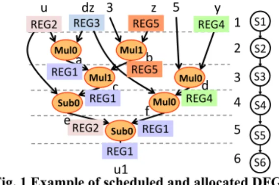
Example 1: The scheduled and allocated data flow graph of ex2 [11] is shown in Fig. 1. The data path behavioral graph G and the state transition graph H are shown in Fig. 2.
<Definition 3: Ignoring of a vertex set>
In a data path behavioral graph G, the ignoring of a vertex set W which is between v and u v, u V, t v t u is to delete all vertices W and all edges connected with the vertices are deleted and to insert an edge (v, u). e E is an output edge of v and f E is an input edge of u. If r(e) = r(f) 0, W can be ignored. r((v, u))=r(e)=r(f), p((v, u))=p(e)=p(f), l((v, u))=1, and h((v, u))={}.
Fig. 1 Example of scheduled and allocated DFG
<Definition 4: Concatenation between vertices>
In a data path behavioral graph G, the concatenation between v and u v, u V, t v t u which are not reachable each other is to delete an output edge e of v and an input edge f of u e, f E, r e r f and to insert an edge (v, u). r((v, u))=r(e)=r(f), p((v, u))=p(e)=p(f), l((v, u))=1, and h((v, u))={}.
<Definition 5: Shortening of an edge>
In a data path behavioral graph G,the shortening of an edge e e E, r e , e and e is to make l(e) smaller.
<Definition 6: Replacement of an edge>
In a data path behavioral graph G, the replacement of an edgev, u to an edge v , u v, u , v , u , v , u E, v, v , u, u′ V, r v , u ) h v, u ) is to delete an edge (u, v) and to insert an edge v , u . r v , u r v , u , p v , u p v , u , v , u , h v , u .
<Definition 7: Insertion of a vertex>
In a data path behavioral graph G, the insertion of a vertex w w V between v and u v, u, w V, t v t w t u is to delete an edge (v, u) and to insert a vertex w and an edge (w, u). If there does not exist a vertex x x V) such that q(w)=q(x) and t(w)=t(x), a vertex w can be inserted. r((w, v)) = r((v, u)), h((w, v))={}, q(w) = q(v), and s(w)=s(v).
<Definition 8: Update of the time of a vertex>
In a data path behavioral graph G, the update of the time for a vertex v (v V is to change t(v).
<Definition 9: Easily testable functional k-time expansion models>
A directed graph pair G , H generated in the following procedures is defined as an easily testable functional k-time expansion model derived from G, H .
G V, E, o, r, p, , h, q, s, t is a directed graph generated by performing the procedures (from pd1 to pd8) for G V, E, o, r, p, , h, q, s, t to satisfy c1, c2, and c3.
S1 S2 S3 S4 S5 S6
u dz
b
3 z 5 y
a c d
u1
2 1
3 4 5 REG2 REG3 REG5 REG4
REG1 REG5
REG1 REG4
REG2 REG1
e f
Mul0 Mul1
Mul1 Mul0
Sub0 Mul0
Sub0
REG1 6
Fig.2 Example of G and H
(pd1) For ∀e E such that p(e)=2 or p(e)=3, edges are selected as detection registers, and the output vertices connected with the selected edges are deleted. Here, detection registers are ones that are connected with primary outputs which can observe fault effects.
(pd2) Ignoring of vertex sets (pd3) Concatenation of vertices (pd4) Replacement of edges (pd5) Shortening of edges (pd6) Insertion of vertices
(pd7) Vertices and edges which are not reachable in input direction to primary inputs or constants are deleted. Vertices and edges which are not reachable in output direction to detection registers are deleted.
(pd8) Update the times of vertices
(c1) For ∀v V such that s(v) = 2 or s(v) = 3, an input edge of v is reachable to vertices corresponding to primary inputs or constants.
(c2) (The number of ∀t v for ∀v V k (c3) In following two conditions, at least one is satisfied. (a) There does not exist w such that t v t w
t u for ∀ v, u v, w, u V, v, u E .
(a) (G’1, H’1)
(b) (G’2, H’2)
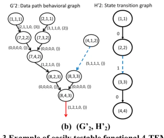
Fig. 3 Example of easily testable functional 4-TEMs
(b) If there exists w such that
t v t w t u for ∀ v, u , (the number of
∀t w for ∀w) +1 = l((v, u)).
H V, E, o, r, p, , h, q, s, t is a directed graph generated by performing the procedures (from pc1 to pc4) for H V, E, s, t, p and G V, E, o, r, p, , h, q, s, t .
(pc1) v V in G′ is the input vertex of the edge corresponding to a detection register, and u V in H′ is the vertex corresponding to a state such that t(v) = t(u). w V in H′ is the output vertex of u and the vertex corresponding to a state such that primary outputs in G′ are observed.
(pc2) For ∀v V in G′ and ∀u V in H, if v such that t v t u , u and the input edge and the output edge of u are deleted. However, if u is the state which primary outputs in G′ are observed, u is not deleted.
(pc3) In H′, let us consider ∀ w, x such that w, x E, w, x, y V, and p w, x . In G , let us consider
∀ v, u such that v, u E, v, w V, t w t v , and t x t u . If o v, u for ∀ v, u , (w, x) is preserved. If o v, u for ∀ v, u , an edge y, x such that t y max t v ) is inserted in H′ and (w, x) is deleted.
(pc4) In H′, assuming that u V is the destination state of v V, t(u) is updated such that t(u)=t(v)+1. If v V does not have an input edge, t(v)=1.
Example 2: Fig. 3 is the example of the two easily testable functional 4-TEMs derived from Fig. 2. ′ of Fig.3 (a) is generated as follows. In G, the output edge of the vertex with (9, 4, 5) is selected as the detection register at pd1, the vertex set which consists of (9, 2, 4) and (9, 4, 4) between (1, 1, 1) and (9, 2, 5) is ignored at pd2, and (7, 4, 2) and (9, 3, 5) are concatenated at pd3. Next, the edge between (1, 1, 1) and (7, 2, 2 ) is replaced with the edge between (2, 1, 1) and (7, 2, 2), and the edge between (2, 1, 1) and (7, 3, 2) is
(0,0,0,0, {}) (2,1,1,0, {3})
(0,0,0,0, {}) (3,1,1,0, {2})
(3,1,3,0, {2})
(1,2,1,0, {})
(0,0,0,0, {}) (5,1,1,0, {}) (4,1,2,0, {3}) (0,0,0,0, {})
(0,0,0,0, {}) (0,0,0,0, {})
(0,0,0,0, {}) (0,0,0,0, {}) (5,1,1,0, {})
(0,0,0,0, {}) (0,0,0,0, {})
(1,2,1,0, {}) (4,1,1,0, {3})
(0,0,0,0, {}) (0,0,0,0, {}) (0,0,0,0, {})
(0,0,0,0, {})
(2,1,1,0, {})
(1,2,1,0, {}) (0,0,0,0, {}) (0,0,0,0, {})
(1,2,1,0, {}) (2,1,3,0, {})
(1,1)
(2,2)
(3,3)
(4,4)
(5,5)
(6,6) 0
0
0
0
0 (,,l,,h) p
(2,1,1)
(1,1,1) (3,5,2) (4,1,1) (5,5,3) (6,1,1)
(8,2,2)
(7,2,2) (7,3,2) (8,3,2)
(7,4,2) (8,4,2)
(7,2,3) (7,3,3) (8,2,3) (8,3,3)
(7,4,3) (8,4,3)
(9,2,4) (9,3,4) (7,2,4) (7,3,4)
(9,4,4) (7,4,4)
(9,2,5) (9,3,5)
(9,4,5)
,, (s,t)
(0,0,0,0, {}) (0,0,0,0, {})
(2,1,1,0, {})
(1,2,1,0, {})
(0,0,0,0, {}) (0,0,0,0, {}) (1,2,1,0, {})
(1,1)
(2,2)
(5,3)
(6,4) 1
1
0
(3,1,1,1, {}) (4,1,1,1, {})
G’1:Data path behavioral graph H’1: State transition graph
(2,1,1) (6,1,1)
(7,2,2) (7,3,2)
(7,4,2)
(9,2,5) (9,3,5)
(9,4,5) (1,1,2)
(0,0,0,0, {}) (2,1,1,0, {3})
(0,0,0,0, {}) (3,1,1,0, {2})
(1,2,1,0, {}) (5,1,1,1, {})
(0,0,0,0, {}) (0,0,0,0, {})
(1,2,1,0, {})
(1,1)
(2,2)
(3,3)
(4,4) 0
1
0
G’2:Data path behavioral graph H’2: State transition graph (2,1,1)
(1,1,1)
(4,1,2) (7,2,2) (7,3,2)
(8,2,3) (8,3,3)
(8,4,3) (7,4,2)
replaced with the edge between (6, 1, 1) and (7, 3, 2) at pd4. Finally, the unnecessary vertices and edges are deleted at pd7, the time when (1, 1, 1) is executed is changed from 1 to 2 and (1, 1, 1) is updated (1, 1, 2) at pd8, and ′ is generated. ′ is generated from ′ and . Since the additional edges are inserted at pd2, pd3, and pd4 in ′ , the edge from (1, 1) to (2, 2) is deleted and the additional edges from (1, 1) to (2, 2) and from (2, 2) to (5,3) are inserted for testing at pc3. ′ of Fig.3 (b) is generated as follows. In G, the output edge of the vertex with (8, 4, 3) is selected as the detection register at pd1, and the vertex set which consists of (8, 3, 2) and (8, 4, 2) between (4, 1, 1) and (8, 3, 3) is ignored at pd2. Finally, the unnecessary vertices and edges are deleted at pd7, the time when (4, 1, 1) is executed is changed from 1 to 2 and (4, 1, 1) is updated (4, 1, 2) at pd8, and ′ is generated. ′ is generated from ′ and . Since the additional edges are inserted at pd2 in ′ , the edge from (2, 2) to (3, 3) is deleted and the additional edge from (2, 2) to (3, 3) is inserted for testing at pc3.
B. Problem Formulation
Inputs: A set of data path behavioral graphs: , , ⋯ ,
A set of state transition graphs: , , ⋯ , The number of time expansions: k
The number of easily testable functional k-TEMs: m Outputs: A set of easily testable functional k-TEMs:
M , , , , ⋯ , , ′ derived from
a set of data path behavioral graphs, , , ⋯ ,
Constraint: Three following constraints have to be satisfied.
(1) |M|
(2) For ∀v V, MAX t v in ′ )
(3) Let be a set of any vertices in ′ corresponding to output terminals for operational units, and let be a set of any edges in ′ corresponding to registers. All operational units in a data path are included in
⋃ . All registers in a data path are included in
⋃ .
Optimization: Maximize COST= ∑ ′ , ′
Eval , α ,
where , , and are coefficients, is the number of additional state transitions for controller augmentation, is the number of operational units controlled by constants,
and is the number of operational units in re-convergence structures. The clause of coefficient expresses the cost of the area overhead for controller augmentation. The clause of coefficient expresses the cost of test generation time. The clause of coefficient expresses the cost of the number of the additional controller inputs for controller augmentation. The clause of coefficient expresses the penalty of testability degradation due to constraints and re-convergence structures.
V. EXPERIMENTAL RESULTS
We evaluated the effectiveness of the proposed method by experiments. High level synthesis benchmark circuits used for experiments are data flow graph (DFG) based circuits named ex2 [11], ex4 [11], and DFCT [12], and control data flow graph (CDFG) based circuits named Sehwa [11], Maha [11], and Kim [11]. Scheduling and binding were performed for high level synthesis benchmark circuits using our in-house behavioral synthesis tool, PICTHY. After that, The RTL circuits which consist of data path and controller were synthesized. The easily testable functional k-TEMs for data paths were generated from state transition graphs and data path behavioral graphs. The controllers were augmented to make the easily testable k-TEMs controllable by adding state transitions and inputs of controllers. The logical circuits were synthesized from the RTL circuits with controller augmentation. Test generation was performed for the logical circuits using STAGY [9] which is our in-house test generation tool using structural TEMs or functional TEMs. Single stuck-at faults were set in the operational units. The proposed method was compared with the three following methods (t1, t2, and t3). (t1) The test generation method using structural TEMs based on original controller functions
(t2) The test generation method using structural TEMs based on original and augmented controller functions (t3) The test generation method using functional TEMs based on original controller functions
(Proposed) The test generation method using functional TEMs based on original and augmented controller functions In t1 and t2, the number of time expansions was 20 for DFG based circuits and was 30 for CDFG-based circuits. In t3 and the proposed method, functional TEMs and easily testable functional k-TEMs were generated such that all state transitions in controllers were executed. Thus, in t3, the numbers of functional TEMs were 1 for ex2, ex4, and DFCT, were 3 for Kim, and were 4 for Sehwa, and Maha. The limit of backtracking was set to 100 for each fault.
The results of the generated easily testable functional
TEMs and the area overhead are shown in Table I. In Table I, “j”, “L”, “m”, “k”, “AST”, and “AOH” denote the number of the data path behavioral graphs, the maximum latency of the functional operations (the number of cycles), the number of the easily testable functional TEMs, the maximum number of the time expansions, the number of the additional state transitions, and the ratio of the area overhead to the whole circuit area, respectively. In Sehwa, the number of time expansions was drastically reduced from 17 to 4 compared with t3. The area overhead for the controller augmentation was as small as 0.9%.The average area overhead for all circuits was as small as 0.62%.
The results of the test generation are shown in Table II. In ex2, only the proposed method obtained 100% fault coverage. In ex4 and DFCT, the fault coverage of t2 and t3 was higher than that of the proposed method. Since the proposed method used many constraints in test generation, the functional operation was restricted. Thus, only a part of data path operated. Therefore, it is considered that faults were not accidently detected by fault simulation. In other methods, many faults in DFG based circuits could be accidentally detected by fault simulation. In Sehwa, t2 and the proposed method could achieve 100 % fault coverage. This result showed that the controller augmentation was effective. The proposed method could generate test sequences about 30 times faster than t2. This result showed that the easily testable functional k-TEMs could drastically reduce the search space to generate test sequences. The proposed method obtained the same results for Maha and Kim. Thus, the proposed method is very effective for CDFG based circuits. As for the length of test sequences, the proposed method is effective for CDFG based circuits.
VI. CONCLUSION
In this paper, we introduced easily testable functional k-TEMs for data paths and proposed a controller augmentation method to make easily testable functional k-TEMs for the data path controllable. We also formulated easily testable functional k-TEMs generation as maximization problem. We confirmed the effectiveness of our proposed method by experimental results using high level synthesis benchmark circuits.
Future work includes evaluating the proposed method for practical circuits and proposing a test generation method for faults in controllers.
REFERENCES
[1] M.C.McFarland, A.C.Parker, R.Camposano, “The high-level synthesis of digital systems”, Proc. IEEE, pp.301-318, 1990. [2] M.T.-C. Lee, W. H. Wolf, and N. K. Jha, “Behavioral synthesis
for easy testability in data path scheduling”, in Proc. Int. Conf. on Computer-Aided Design, pp.616 -619 , 1992.
[3] M.T.-C. Lee, W. H. Wolf, and N. K. Jha, “Behavioral synthesis for easy testability in data path allocation”, in Proc. Int. Conf. Computer Design, pp. 29 -32 , 1992.
[4] M.T.-C. Lee, N. K. Jha , and W. H. Wolf, “Behavioral synthesis for highly testable data paths under the non-scan and partial scan environments”, in Proc. Design Automation Conf., pp.292-297, 1993.
[5] L.M. FLottes, B. Rouzeyre, L. Volpe,” A CONTROLLER RESYNTHESIS BASED METHOS FOR IMPROVING DATAPATH TESTABILITY”, in Proc. Int. Symp. on Circuits and Systems, pp. 347 -350, May 2000.
[6] W.T.Cheng, “The back algorithm for sequential test generation” , in Proc. Int. Conf. on Computer Design, pp. 66-69, 1988.
[7] T.M. Niermann and J.H.Patel, “HITEC: A Test Generation Package for Sequential Circuit”, in Proc. European Design Automation Conf., pp.214-218, Feb.1991 .
[8] H. Fujiwara, H. Iwata, T. Yoneda, and C. Y. Ooi, “A Nonscan Design-for-Testability Method for Register-Transfer-Level Circuits to Generate Linear-Depth Time Expansion Models”, IEEE Trans. On Computer-Aided Design of Integr. Circuits Syst., pp.1535-1544, Vol. 27, No. 9, 2008.
[9] T. Hosokawa, T. Hayakawa, and M. Yoshimura, “A Comprehensive Functional Time Expansion Model Generation Method for Datapaths Using Controllers” , in Proc. Workshop on RTL and High Level Testing, pp.131-138, 2010.
[10] K. Sugiki, T. Hosokawa, and M. Yoshimura,”A Test Generation Method for Datapath Circuits Using Functional Time Expansion Models ”, in Proc. Workshop on RTL and High Level Testing , pp.39 -44, 2008.
[11] M.T.-C.Lee, “High-Level Test Synthesis of Digital VLSI Circuits”, Artech House Publishers, 1997.
[12] I. G. Harris and A. Orailoglu ,“Testability Improvement in High-Level Synthesis Through Reconvergence Reduction”, in Proc. the Asilomar Conference on Signals, Systems and Computers, pp.1919-203 ,1996.
Table 1. Experimental results of functional k-TEM
Table 2. Experimental results of test generation
. . . .
. . . .
. . . .
a . . . .
aa . . . .
. . . .
a a % A
A A %
. . .
a .
aa .
.