Scale invariance vs conformal invariance
Yu Nakayama,
California Institute of Technology, 452-48, Pasadena, California 91125, USA
Abstract
In this review article, we discuss the distinction and possible equivalence between scale invariance and conformal invariance in relativistic quantum field theories. Under some technical assumptions, we can prove that scale invariant quantum field theories in d = 2 dimension necessarily possess the enhanced conformal symmetry. The use of the conformal symmetry is well appreciated in the literature, but the fact that all the scale invariant phenomena in d = 2 dimension enjoy the conformal property relies on the deep structure of the renormalization group. The outstanding question is whether this feature is specific to d = 2 dimension or it holds in higher dimensions, too. As of January 2014, our consensus is that there is no known example of scale invariant but non-conformal field theories in d = 4 dimension under the assumptions of (1) unitarity, (2) Poincar´e invariance (causality), (3) discrete spectrum in scaling dimension, (4) existence of scale current and (5) unbroken scale invariance in the vacuum. We have a perturbative proof of the enhancement of conformal invariance from scale invariance based on the higher dimensional analogue of Zamolodchikov’s c-theorem, but the non-perturbative proof is yet to come. As a reference we have tried to collect as many interesting examples of scale invariance in relativistic quantum field theories as possible in this article. We give a complementary holographic argument based on the energy-condition of the gravitational system and the space-time diffeomorphism in order to support the claim of the symmetry enhancement. We believe that the possible enhancement of conformal invariance from scale invariance reveals the sublime nature of the renormalization group and space-time with holography.
This review is based on a lecture note on scale invariance vs conformal invariance, on which the author gave lectures at Taiwan Central University for the 5th Taiwan School on Strings and Fields.
Contents
1 Introduction 4
1.1 Physical applications we have in mind . . . 8
1.2 Organization of the review and conventions . . . 12
2 Statement of the problem 14 2.1 Conformal algebra as maximal bosonic space-time symmetry . . . 14
2.2 Local field theory realization . . . 15
2.3 Space-time symmetry and energy-momentum tensor . . . 16
2.4 Unitarity, causality and discreteness of spectrum . . . 18
2.4.1 Consequence of scale invariance alone . . . 21
2.4.2 Consequence of conformal invariance . . . 22
2.5 Formulation of the problem . . . 23
3 Energy-momentum tensor and renormalization group 25 3.1 Schwinger functional . . . 25
3.1.1 Promoting coupling constants to background fields . . . 25
3.1.2 Curved background . . . 26
3.2 Weyl Anomaly . . . 27
3.3 Trace of energy-momentum tensor in perturbatively renormalizable theory . . . 30
3.3.1 Interacting theories and renormalization group . . . 30
3.3.2 Ambiguities in local renormalization group . . . 32
3.3.3 Anomalous dimensions and global Callan-Symanzik equation . . . 34
3.4 Computation of trace of energy-momentum tensor . . . 36
3.5 (Redundant) conformal perturbation theory . . . 39
4 Examples 43 4.1 Free theories . . . 43
4.2 Interacting theories . . . 45
4.3 More examples . . . 49
4.4 Theory without action . . . 53
4.5 Controversial examples . . . 55
5 Proof in d = 2 dimension 57 5.1 Zamolodchikov-Polchinski theorem . . . 57
5.2 Canonical scaling of Tµν . . . 59
5.3 Alternative approach . . . 60
5.3.1 Simple alternative derivation . . . 60
5.3.2 Averaged c-theorem . . . 62
6 Conjecture in d > 2 64 6.1 Scale invariance vs Conformal invariance . . . 64
6.2 Cardy’s conjecture (a.k.a “a-theorem”) . . . 64
6.3 Scale invariant energy-momentum tensor . . . 66
7 Local renormalization group and perturbative proof in d = 4 dimension 68
7.1 Local renormalization group . . . 68
7.2 Mixing of energy-momentum tensor with scalars and improvement . . . 71
8 Nonperturbative aspects, a-theorem, and dilaton scattering amplitudes 73 8.1 a-maximization . . . 73
8.2 Proof of weak a-theorem . . . 73
8.3 Scale vs Conformal in d = 4 dimension . . . 78
8.3.1 Some technical comments on possible cancellation . . . 81
8.3.2 Space-time dependent coupling constant counterterms . . . 83
8.4 n− n dilaton scattering amplitude . . . 85
8.5 Physical reason why scale invariance implies conformal invariance in perturbative fixed point . . . 87
9 Other dimensions or less symmetry 90 9.1 Summary of the situations in other dimensions . . . 90
9.2 Possible directions . . . 91
9.2.1 F-theorem in d = 3 dimension . . . 91
9.2.2 In relation to entanglement entropy . . . 92
9.2.3 Local renormalization group in other dimensions . . . 94
9.3 Reduced symmetry . . . 95
10 Holography 100 10.1 AdS/CFT and holography . . . 100
10.2 Holographic c-theorem . . . 103
10.3 Scale vs Conformal from holography . . . 108
10.3.1 Holographic counterexample 1: null energy violation . . . 111
10.3.2 Holographic counterexample 2: foliation preserving diffeomorphic theory of gravity112 10.4 Beyond classical Einstein gravity . . . 114
10.4.1 Higher derivative corrections . . . 114
10.4.2 Quantum violation of null energy condition . . . 116
10.5 Reduced symmetry . . . 118
10.6 Further thoughts . . . 120
10.6.1 More on literature . . . 120
10.6.2 Final Project . . . 121
10.6.3 Derivation of holography from local renormalization group? . . . 122
11 Conclusions 124 Appendix A Useful formulae and miscellaneous topics 126 Appendix A.1 Weyl transformation . . . 126
Appendix A.2 Energy-momentum tensor correlation functions . . . 126
Appendix A.3 Local Wess-Zumino consistency condition . . . 128
Appendix A.4 Analytic properties of S-matrix . . . 130
1. Introduction
In late 1970s, there was a legendary international conference at Dubna, a city in the former Soviet Union. The theme of the workshop was scale invariance in physics. The organizer was N. N. Bogoli- ubov, who is one of the founders of the renormalization group and who first introduced the concept of scale invariance in quantum field theory. His influence on renormalization group, among other nu- merous contributions to mathematical physics, was enormous. For example, K. Wilson later recalls at the Nobel lecture that it was one mysterious chapter in his famous textbook [5] that mesmerized him when he was a PhD student and eventually led him to the later study of the renormalization group.
At one point of the conference after the plenary session for scale invariance, one western physicist asked a question, which KGB might have called “provocative” in those days: What is the difference between scale symmetry and conformal symmetry? The speaker got stuck and hesitated to answer. The chairman of the session, Bogoliubov, however, immediately took the microphone and spoke with dignity “There is no mathematical difference, but when some young people want to use a fancy word they call it Conformal Symmetry”. One young eastern physicist could not stand this answer, stood up and yelled “15 parameters!”. The yell echoed but did not reach. The adjournment of the meeting was quickly announced.
The name of the eastern young physicist is A.A Migdal, who is one of the earlier advocates of the use of conformal invariance in theoretical physics. This anecdote can be found in his biography
“Ancient history of conformal field theory” [1]. The aim of this review article is first to understand the mathematical as well physical idea behind this 40 year long debate about the relation between scale invariance and conformal invariance. As we go along, we will see the amusing twist and turn: mathematically what Migdal yelled was correct, but physically what Bogoliubov answered may be true! Under some mild assumptions, scale invariant quantum field theories always seem to be conformal invariant! To appreciate the statement better, we have to start with the distinction between scale invariance and conformal invariance.
In elementary school, we learn a rectangle is not a square. In graduate school, we, however, learn (?) scale invariance is conformal invariance. In the era of AdS/CFT, everybody touts conformal invariance, so without much reflection we are somehow accustomed to the “belief” that scale invariant quantum field theories show conformal invariance. Let us, however, pose here and ask ourselves the questions: has it been proved? Are we really sure our beloved N = 4 supersymmetric Yang-Mills theory is conformal invariant? Are we just some young people who want to use a fancy word?
Of course scale invariance does not imply conformal invariance at least at the level of the superficial mathematical definition. Otherwise, we do not need two different names for the identical concept. However, our nature may be more beautiful than we naively expect. This hidden beauty of the nature is the essential reason why we are interested in the question about the relation between scale invariance and conformal invariance. Our ultimate goal of the review is to understand the mysterious symmetry enhancement in quantum field theories and gravitational systems.
Indeed, such a symmetry enhancement may happen. In general relativity, for instance, there is a famous theorem by Israel [2] that states all axisymmetric static black holes must be spherically symmetric in d = 4 dimension (i.e. Schwartzshild black hole solution) as vacuum solutions of Einstein’s equation. This is a symmetry enhancement from the axisymmetry to the spherical symmetry due to the dynamics of the classical gravitational system. Presumably it has a deep quantum gravitational origin. The black hole has no hair, and any classical probe cannot distinguish the microscopic degrees of freedom. We expect that the symmetry enhancement does not occur with no good reason.
Scale invariance is ubiquitous in our nature. We can easily find them in our daily lives. The
coastline, snowflakes, lightening, and stock charts, all show scale invariance or fractal structures. Even at a supermarket we can find a vegetable called roman cauliflower (a.k.a broccoli romanesque), which shows a beautiful discrete scale invariant structure.1 The (discrete) scale invariance here is realized as a self-similarity: if we look at the same system closer or further away, it looks similar. Does our society show a self-similar organization structure? The repetitive structure begs the question: is there any fundamental component in such a self-similar or scale invariant object? Or, is the self-similar structure itself the fundamental organizing principle?
The most notable application of the scale invariance in theoretical physics is the renormalization group flow. One of the central dogmas in the 20th century physics was Wilson’s renormalization group (see e.g. [3]). In a plain word, his idea of the renormalization group is a successive application of scale transformation and coarse graining. If we are interested in the long range universal physics, we can then integrate out the short-range degrees of freedom that might show non-universal dynamics. Afterwards we can talk about the effective theory of the long range degrees of freedom by keeping only relevant degrees of freedom of the theory and focusing on the relevant parameters. All the detailed short range information is judiciously encoded in the process of the renormalization of the relevant parameters.
Schematically, renormalization group transformation is realized as the path integral form: e−Seff[ ˜Φ;g(Λ)] =
∫ Λ0
Λ DΦe
−S0[Φ;g(Λ0)] (1.1)
where Λ is the renormalization scale. Such path integrals appear either in quantum field theories or in the statistical mechanical ensembles. In either situations, we integrate out the “high energy degrees of freedom” from the scale between Λ0 and Λ contained in a field Φ by keeping only the low energy mode below Λ. We expect that when we take Λ sufficiently small, there are only a few universal parameters that will characterize the system. The success of the idea of the renormalization group transformation explains why we can understand our world with sufficient accuracy even without knowing the most detailed elementary microscopic physics (e.g. string theory?). Without exaggeration, this is how our standard model works in elementary particle physics, how Einstein’s general relativity works in gravitational physics, how the hydrodynamics works in such a way that our airplane flies, and how the idea of universality of the statistical mechanics work in condensed matter physics.
From Wilson’s renormalization group viewpoint, it may be natural that we would expect a scale invariant fixed point in the infrared (IR) limit. The intuition is that if we encounter any non-trivial energy scale, we can simply integrate out the corresponding degrees of freedom. Eventually, there should be no scale at all! As a consequence, the universality class of the long range behavior in quantum field theories or many body systems is characterized by the fixed point of the renormalization group flow. This idea has a great success in particular in d = 2 dimension, dimension where the universality combined with conformal invariance made it possible to classify the critical phenomena.
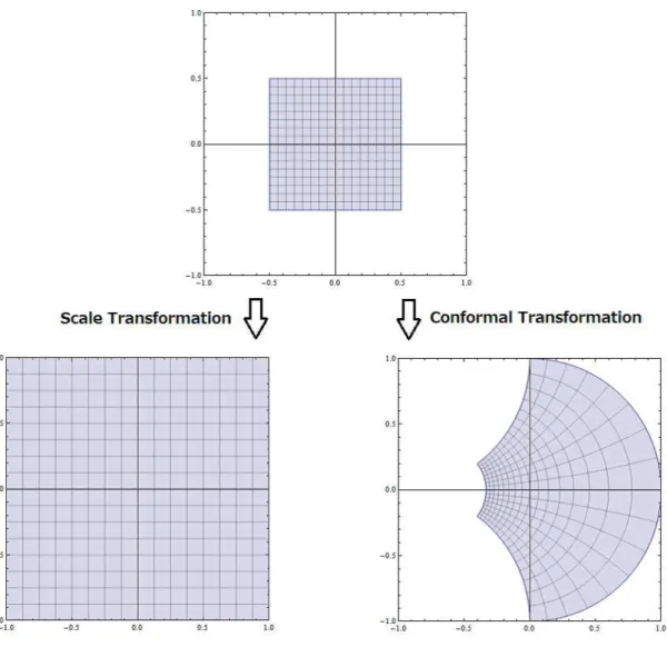
Conformal invariance is the other leading actor of this review article. What is conformal invari- ance? While we will describe the mathematical definition of the conformal invariance momentarily, an intuitive idea can be guessed from the root: “con-formal” comes from a Latin word conformalis “hav- ing the same shape”. It is the transformation that leaves the size of the angle between corresponding curves unchanged. Such transformations are more general than the scale transformation. See fig 1. In d = 4 dimension, the parameter of the conformal transformation is 15 rather than 11 of Poincar´e + scale symmetry.
1It is good with pasta, in particular with oil-based source.
Figure 1: We see a graphical distinction between scale invariance and conformal invariance in d = 2 dimension. Our perception is approximately invariant under scale transformation but not invariant under conformal transformation. Do you think conformal transformation keeps the “same shape”?
Therefore there is no a priori reason why a given scale invariant system must show conformal invariance. Nevertheless, as we mentioned at the beginning, there should be a reason why theoretical physicists in our generation have not made a clear distinction in our everyday research. We believe it is because we have empirical knowledge that almost all scale invariant quantum field theories that we know show conformal invariance so there is no point in emphasizing it in our textbooks. Do we have to talk about unicorns or dragons in zoology lectures or in textbooks (even though they might exist in principle due to our limited knowledge)?
But it is still a mystery: why does scale invariance have to accompany conformal invariance? The aim of this review article is to uncover the puzzle behind the enhancement of conformal invariance from scale invariance. As we will see, the underlying reason must be related to a deep property of the renormalization group flow. In particular, the notion of irreversibility of the renormalization group flow and counting degrees of freedom will play a crucial role in our discussions.
The idea of irreversibility of the renormalization group flow can be understood in an intuitive way: as mentioned, the renormalization group flow is accompanied with a kind of coarse graining. We lose
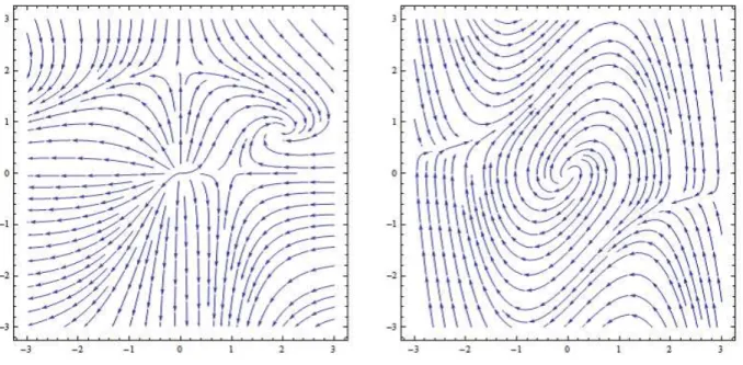
information along the flow. It is very counterintuitive if the renormalization group flow shows a cyclic or chaotic behavior (although it was envisaged by the pioneers [4][5]). See fig 2 for illustration. The field theory understanding of this coarse graining is supported by the so-called “c-theorem” that dictates there exists a function (called “c”-function) that monotonically decreases along the renormalization group flow. Roughly speaking, this function counts the degrees of freedom at a given energy scale. If such a function exists, the cyclic or chaotic behavior in renormalization group flow cannot occur. In relativistic quantum field theories in d = 2 dimension, there is a proof that such a function indeed exists and the renormalization group flow is irreversible [6].
Figure 2: We show artificially generated examples of (possible?) renormalization group flow. The left hand side contains UV fixed point as well as IR fixed point. The right hand side shows a cyclic behavior with UV fixed point.
As we will see, scale invariant but non-conformal field theories are intimately connected with the possibility of such a cyclic or chaotic behavior in the renormalization group flow. At least this is the case within perturbation theory in d = 4 dimension as first emphasized in [7]. There is a clear tension between them. The above mentioned proof in d = 2 dimension of the irreversibility of the renormalization group flow implies that scale invariance must be enhanced to conformal invariance in d = 2 dimension. In this review article, we would like to report the current status of the situations in higher dimensions. Unfortunately, as of January 2014, there is no compelling non-perturbative proof that scale invariance is enhanced to conformal invariance in higher dimensions with no counterexamples reported so far under some reasonable assumptions. However, our accumulated knowledge of the subject in recent years in line with the development of the higher dimensional analogue of the c- theorem may suggest that the complete proof will be close by.
To look for a non-perturbative evidence, we will study the holographic argument. This is the second aim of this review article, which was mainly developed by the present author. Holographic principle is by far the most profound but conjectural principle that connects non-gravitational quantum physics and the corresponding (quantum) gravity. It has a beautiful concrete realization known as AdS/CFT correspondence, and we have culminating evidence that it is true. With the holographic principle in mind, our idea is to explore the hidden side of the quantum field theories from the analysis
in gravitational backgrounds. According to the AdS/CFT correspondence, the classical gravity will describe a certain strongly coupled limit of the dual quantum field theories, and it is expected that it provides non-perturbative understanding of them.
As we have already mentioned in the black hole example, gravitational systems show their own symmetry enhancement mechanism. We conjecture that the consistency of the quantum gravity is encoded in the consistency of the renormalization group flow through the holographic equivalence, and vice versa. The c-function associated with the renormalization group flow can be viewed as “entropy” of the gravitational system, which should be monotonically decreasing along the evolution. Along the same line of reasoning, we will argue that it is reasonable that scale invariant holographic configurations show the enhanced enhanced symmetry corresponding to conformal invariance. Indeed, we will see that we can provide a holographic proof of the statement based on a certain energy-condition.
At the same time, we would like to ask some pertinent questions in quantum gravity. What would be the fundamental mechanism to exclude seemingly pathological geometries from quantum gravity such as superluminal propagation of information, closed time-like curves, and so on? We believe that the consistency of the renormalization group flow e.g. absence of the limit cycle or chaotic behavior would give a hint to understand the fundamental aspects of quantum geometry and quantum gravity through the holography. Our earlier attempt to discuss the issue from the holographic approach is summarized in a review paper [8].
There was a debate whether scale invariance without conformal invariance is possible or not in d = 4 dimension over the last couple of years, but we are happy to announce that we converge to the point our holographic argument predicts [9][10][11]. However, the complete proof is yet to come. We wish the complete field theory proof would appear soon to make this review article partly obsolete. 1.1. Physical applications we have in mind
Suppose we could show that scale invariant quantum field theories necessarily possess the enhanced symmetry of conformal invariance. What could we learn? What would be the practical benefit of con- formal invariance compared with the mere scale invariance? Are there any real applications of con- formal invariance relevant for our understanding of physical phenomena in nature? Or, alternatively, is there any physics which relies on scale invariance without conformal invariance? Before going into the technical analysis of the relation between scale invariance and conformal invariance from section 2 on, we would first like to show how the distinction and possible equivalence between scale invariance and conformal invariance plays an important role in various examples in condensed matter physics, high energy physics, gravitational physics, as well as other arenas of physics and beyond. The list is far from complete, so we would like to encourage interested readers to look for possible further applications.
• Critical phenomena:
Boiling water may be the first example of phase transition we learn in the science classroom during our elementary education. The phase transition under the normal pressure we typically experience on earth is first order. However, it is known that if we tune the pressure, the thermal transition of water can be second order (at T = 273.16K and P = 0.61kPa). The second order phase transition there is known as an example of critical phenomena (see e.g. [12] for a review). A surprising fact is that the second order phase transition of the water shows the universality. It means that various critical exponents take the universal values: the jump of the density near the critical temperature Tc for example shows
δρ(T )∼ (T − Tc)β (1.2)
where β∼ 0.325, and the specific heat shows
C ∼ (T − Tc)−α (1.3)
where α∼ 0.11. These numbers are precisely same as that of the d = 3 dimensional Ising model at the critical point, where for example the density ρ in the above water example is replaced by the spontaneous magnetization, up to experimental/numerical errors. One of the goal of the theoretical physics is to understand these universal properties associated with the critical phenomena. How do they occur emergently and why do they show the universality?
The crucial observation is that at the critical point, the so-called “scaling hypothesis” applies [13], which means that the thermodynamic quantities show the scaling behavior. As already mentioned, the best way to understand the critical behavior with the scale invariance would be the renormalization group. The second order phase transition and the associated critical phenomena are characterized by the scale invariant fixed point of the effective Hamiltonian (or free energy).
The scaling hypothesis alone cannot determine the critical exponent while it may give some relations among them. Here is the power of conformal invariance. Suppose that the critical phenomena are classified by the conformal invariant fixed point. Then the classification of the critical phenomena is equivalent to the classification of conformal field theories. For instance, in d = 2 dimension, a complete classification (for small central charge, relevant for condensed matter applications) of the conformal field theories is possible [65] , and the critical exponent is solely determined by the constraint from the conformal invariance.
It is very likely that the critical exponents of the higher dimensional critical phenomena are controlled by the dynamics of conformal field theories as in d = 2 dimension. Indeed, the recent development (which we will briefly mention in section 2.4.2) shows that the critical exponents such as (1.2) (1.3) are completely consistent with the conformal hypothesis. It is this “conformal hypothesis” than the mere scaling hypothesis that enables us to compute the critical exponents by using the constraint from the conformal symmetry.
It is therefore of theoretical as well as practical importance to understand under which con- ditions we expect the conformal invariance in critical phenomena. Our study of the relation between scale invariance and conformal invariance is essential because the definition of the criti- cal phenomena and the simple renormalization group argument by themselves do not imply the emergence of the conformal invariance (at least without further thoughts). Nevertheless, we are led to the belief that the conformal hypothesis is more or less valid through our experience. One of the final goals of this study is to give a firm basis of this belief.
• Particle physics:
Quantum field theories are foundation of particle physics. The notion of approximate or asymp- totic scale invariance in quantum field theories describing the elementary particles played a significant role in understanding the high energy properties of QCD, which is asymptotic to the trivial Gaussian scale invariant fixed point (massless free field theories) in the ultraviolet (UV) limit [14][15]. The free Gaussian fixed point there turns out to be also conformal invariant. A slight violation of the scale invariance is known as the Bjorken scaling in QCD phenomenol- ogy [16]. Historically speaking, the conformal symmetry itself was discovered in the study of Maxwell theory of electromagnetism, which is probably the best known example of conformal field theories realized in nature.
The scale invariance is tightly related to massless properties of the quantized field. It is obvious that the mass “scale” will break the scale invariance. However, it is slightly non-trivial that clas- sical scale invariance will be typically broken in quantum field theories due to the renormalization group effect. Thus, the emergence of scale invariance in particle physics is quite non-trivial. We should again emphasize that the conformal invariance is stronger than the mere scale invariance at this point. Although related, the massless field theories (even if we ignore the interaction) do not necessarily possess conformal invariance. A good example is the Einstein gravity with zero cosmological constant. At the linearized level, it describes the massless scale invariant graviton, but the theory is not conformal invariant off-shell (while the dispersion of the on-shell graviton is conformal invariant).
In some beyond-the-standard-model scenarios, the existence of non-trivial scale invariant fixed points plays some important roles (see e.g. [17] for a review). Our standard model has the so-called hierarchy problem. The weak-energy scale is more than fifteen digit smaller than the Planck scale, and the naive power-counting suppressed by the Planck scale (or any other high energy scale) gives various constraints on the model building without allowing fine-tuning. One typical idea to use the scale invariant non-trivial fixed point as a part of the model building tools is to rely on the “anomalous dimensions” of various operators to deviate from the naive engineering dimensional counting.
However, the extra constraint from the conformal invariance may give further restrictions on the possible amount of anomalous dimensions [18]. The structure of the renormalization group such as the irreversibility may further restrict the possibility. On the other hand, if the scale invariance without conformal invariance were allowed, the constraint could be relaxed with a slight loss of predictive powers. It relies on our philosophical viewpoint which is better (i.e. generalization vs predictive power), but the discussion would be moot for the latter possibility of using scale invariant but non-conformal field theories if it turns out that such theories do not exist at all.
There is also a speculative idea that our standard model may be embedded in the scale invariant UV fixed point. A partial implementation of the idea led to the prediction of 126 GeV Higgs mass [19] (see also [20]). The idea is tightly related to the asymptotic safety scenario, which we would like to turn next in the context of gravity.
• Cosmology and gravitational physics:
There are two major directions to apply scale invariance in cosmology and gravitational physics. The first one is the possibility of asymptotic safety in quantum gravity [21] (see e.g. [22] for a review). The conjecture is that although Einstein gravity is non-renormalizable in the power- counting sense and it is strongly coupled in the ultraviolet, it may have a non-trivial UV fixed point and the lack of the predictive power in non-renormalizable theory may be circumvented by assuming that we are on the flow emanating from this hypothetical UV fixed point of quantum gravity. Obviously, the UV fixed point must be scale invariant. It is less obvious if such a fixed point (if any) would show the conformal invariance. As we will discuss in this review, the gravitational theory (either scale invariant or conformal invariant) is special and does not satisfy the usual assumptions we would make when we talk about the enhancement of conformal invariance from scale invariance.
Another possible application of scale invariance in cosmology is the primordial fluctuations in cosmic microwave background [23]. The fluctuation of the cosmic microwave background is
known to be nearly scale invariant from the observational data, and one explanation is from the approximate de-Sitter invariance during the inflation. The crucial point is the de-Sitter invariance could predict the enhanced (nearly) conformal invariant spectrum rather than the mere scale invariant spectrum [24]. So far, observationally we have no evidence for or against the enhanced conformal invariance in the cosmic microwave background. It is very interesting to see if this hypothetical conformal invariance could be observed in the cosmic microwave background in the study of the higher point functions in the tensor mode. At the same time, it would be very interesting if we could construct a cosmological model that predicts only the scale invariance without the enhanced conformal invariance. Based on the holography, it may be related to the possibility to have scale invariant but non-conformal field theories in d = 3 dimension.
• String theory:
The foundation of the worldsheet formulation of the first quantized string theory is a conformal field theory (see e.g. [122][123] for a review). In order to get rid of the space-time ghost and construct the consistent loop amplitudes, it is not enough to have scale invariance: the worldsheet theory must possess the conformal invariance. The distinction between scale invariance and conformal invariance is crucial, and there can be a target space which is not consistent as a string background due to the lack of the worldsheet conformal invariance although it is scale invariant. Note that the situation is a slightly peculiar because the general theorem of enhancement of conformal invariance from scale invariance in d = 2 dimension does not apply here because the worldsheet theory violates some of the assumptions made.
As we have already mentioned in the introduction the holography is a novel idea to understand the nature of strongly coupled quantum field theories from gravitational analysis. It was origi- nally developed in the string theory by connecting the symmetry of the AdS space-time and the symmetry of the conformal field theories. Here, the conformal invariance is taken for granted. In this review, we would like to ask the question why and how the holography relies on the underlying conformal invariance of the dual field theories for the consistency. At the same time, we would like to reveal the nature of the space-time from the possible constraint on the dual field theories.
• Biology, economy, human behavior etc:
There are many other arenas of science in which we would encounter scale invariance without conformal invariance. As we have already mentioned in the introduction, in our daily lives there is no shortage of scale invariant phenomena. For another amusing example, Zipf’s law [25] predicts that the frequency of the appearance of words in this review (say, the most common word “the” gets a rank r of 1 and ”broccoli” among others would get the lowest rank) shows the scaling law Q(r) = F r−1/α. Here α measures the richness of one’s vocabulary. As far as the author knows, there is no conformal extension of this observation.
There are two different categories here. In the first case, there is no obvious group theoretic way to extend the scaling symmetry to conformal symmetry. In this case, we can easily explain the non-enhancement of symmetry from scale invariance: simply we cannot do it. Presumably, the stock market economy, which shows power-law scaling behavior falls in this category while there is a possibility of conformal invariance in bond market because it may be described by a free string action (see e.g. [26] and reference therein). The second case, which is more non-trivial and is
similar to the quantum field theory examples so far, is that although the algebraic enhancement of the conformal symmetry from scale invariance is possible, in reality it does not show it. Let us only mention one example: human perception of visionary. Our visual perception is approximately Euclidean invariant as well as scale invariant (so there is a group theoretic chance of enhancement to conformal invariance), but actually we know it is not conformal invariant. If it were conformal invariant, we would not perceive the right panel of Figure 1 as somewhat distorted compared with the left one! Indeed, as we will mention in this review article, there may be a field theoretic understanding of human perception based on scale invariant but non- conformal field theories [93][94][95] as we mentioned in the introduction.
1.2. Organization of the review and conventions
This review is based on a lecture note on scale invariance vs conformal invariance, on which the author gave lectures at Taiwan Central University for the 5th Taiwan School on Strings and Fields. Originally, we had three lectures, and the plan was as follows. In Lecture 1, we began with the definition of scale invariance and conformal invariance, and gave criteria to distinguish between the two. Then we showed various examples of scale invariant systems with or without conformal invariance. In Lecture 2, we tried to give a field theoretic argument why scale invariant phenomena typically show enhanced conformal invariance under several assumptions. In Lecture 3, we gave holographic discussions on the distinction and showed possible enhancement from scale invariance to conformal invariance from the properties of the space-time dynamics.
In this review article, we have reorganized the lectures into 11 sections for a more coherent and self-contained presentation. Lecture 1 corresponds to section 2,3, and 4. Lecture 2 corresponds to section 5,6,7,8, and 9. Lecture 3 corresponds to section 10. Of course, we did not cover everything presented here in the lectures, so the review is significantly expanded compared with what the author discussed in the school. We have also added more recent developments after the school to catch up with the rapid pace of the researches in this field.
Before going into the main discussions, we would like to summarize the basic conventions of the review for future reference. We also provide some small tips for the readers how to read the review.
• As broader audience in mind, let us fix our notation for the space-time dimensionality. When we say d-dimension, it means either d-dimensional Euclidean (statistical) system, or relativistic d-dimensional space-time which is given by d− 1 dimensional space and 1 dimensional time. µ = 0, 1, 2· · · d − 1 refers to Lorentz index with the Minkowski metric ηµν = (− + + · · · ). We also work in the Euclidean signature field theories with no particular mentioning of Wick rotation2 xd= ix0. In the Euclidean signature, we use µ = 1, 2· · · d with the Euclidean metric δµν = (+ + +· · · ). The antisymmetrization of the tensor indices is represented by [IJ], and the symmetrization is represented by (IJ). Only when we discuss field theories in d = 2 dimension, we will use the complex coordinate which will be explained in section 5.1.
• In section 10, we add the extra holographic coordinate and use M = 0, 1, · · · d − 1, r or M = 0, 1,· · · d−1, z referring to d+1-dimensional space-time coordinate. We also work in the Euclidean signature as above.
• We use the natural unit: ℏ = c = 1. In section 10, we further assume the Planck constant κd= 1.
2With this regards, we will not discuss some subtle aspects of the global conformal transformation in Minkowski space-time. See section 4.5.
• Otherwise stated, the summation convention of Einstein is used (e.g. AµBµ≡∑µAµBµ). The
coordinate indices are raised and lowered with an appropriate metric gµν. Such a “metric” may or may not be naturally available when tensor indices take the value in more abstract spaces such as “coupling constant spaces”, and we will be explicit about raising and lowering indices then. □ = DµDµ denotes the Laplacian (or D’Alembertian), and in flat space-time it is given by ∂µ∂µ. The use of □ is not restricted to d = 4 in this review article. In some obvious cases without confusion, we even omit the summation conventions: e.g. x2 = xµxµ.
• Spacetime argument x in field variables such as a scalar field Φ(x) is sometimes omitted as Φ to avoid the clumsy expressions when the space-time dependence is not important.
• Our metric and curvature convention is same as that of Wald’s textbook [27]. See Appendix A.1 for more about our conventions.
• In most of the sections dealing with interacting quantum field theories, we assume fields appear- ing in various formulae are all finitely renormalized, and we typically put the suffix 0 otherwise. Although we do give some basic explanations of the renormalization procedure in the review article, it is beyond our scope to perform the explicit renormalization program, and we refer to textbooks (e.g. [28],[29],[30][31]). Unfortunately, at a certain point, we have to go beyond the textbook treatment because the distinction between scale invariance and conformal invariance is so subtle. We hope interested readers will find reference provided throughout the review article useful and fill the gap if necessary.
• At many places, we state that the renormalization group flow is a quantum effect. In the (classical) statistical systems, It should be understood that the effect is induced by the statistical fluctuation. They are equivalent up on Wick rotation.
• When we talk about quantum gauge theories, the gauge fixing procedure will be always implicit. After the gauge fixing, we have to add various terms both in the action and the energy-momentum tensor. However, all these terms (that could violate scale invariance or conformal invariance) are BRST trivial, so the physical discussions will not be affected.
• We do not cover various techniques in conformal field theories developed in particular in d = 2 dimension. We refer to [32][33] and references therein. We also refer to the lecture note [34] for a complementary approach in higher dimensional conformal field theories.
• We try to avoid spinors and supersymmetry as much as possible. In some advanced sections, we assume some basic knowledge (e.g. γµ denotes the Dirac gamma matrix). For supersymmetry, we refer to textbooks [35][36] and a lecture note [37]. In various symbolic formulae such as a field variation δSδϕ, we implicitly pretend as if ϕ were bosonic and suitable modifications are necessary for anti-commuting fermionic fields.
• The discussion on the holographic approach in section 10 is relatively independent. The other sections are self-contained within field theory arguments. Those who are not interested in holog- raphy can skip section 10 entirely. On the other hand, although understanding of section 10 requires some basic facts presented in the earlier sections, one may directly start with section 10 to grasp the holographic approach. In the latter case, we also recommend [8] for reference.
• Minor revisions will be updated at https://sites.google.com/site/scalevsconformal/
2. Statement of the problem
The aim of this section is to formulate the statement of the problem on the relation between scale invariance and conformal invariance. We begin with the mathematical distinction between scale invariance and conformal invariance, and then we proceed to discuss the criteria to distinguish them in quantum field theories. As we will argue in section 2.3, in local quantum field theories, the criteria are stated as a property of the energy-momentum tensor. Our discussions in this section are restricted to the case in flat Minkowski or Euclidean space-time, but in section 3, we will learn that the problem is better understood in the curved background with more general background sources.
2.1. Conformal algebra as maximal bosonic space-time symmetry
In special relativity, we postulate the Poincar´e algebra as the fundamental symmetry of our space- time:
i[Jµν, Jρσ] = ηνρJµσ− ηµρJνσ− ησµJρν+ ησνJρµ i[Pµ, Jρσ] = ηµρPσ − ηµσPρ
[Pµ, Pν] = 0 . (2.1)
Pµis the translation generator and Jµνis the Lorentz transformation generator. In quantum mechan- ics, they are realized by Hermitian operators acting on a given Hilbert space. The representation of Poincar´e algebra in terms of particles will naturally lead to the formalism of the quantum field theory [30].
For a massless scale invariant theory, one can augment this Poincar´e algebra by adding the dilata- tion generator D as
[Pµ, D] = iPµ
[Jµν, D] = 0 . (2.2)
We use the terminology “dilatation” and “scale transformation” interchangeably throughout the re- view. The representation theory of the Poincar´e algebra augmented with the dilatation naturally leads to the notion of unparticles [39][40]. The theory of unparticles sometimes relies on a delicate difference between scale invariance and conformal invariance (see e.g. [41]).
The generalization of the Coleman-Mandula theorem [42][43] asserts (for d≥ 3) that the maximally enhanced bosonic symmetry of the space-time for massless particles is obtained3 by adding the special conformal transformation Kµ:
[Kµ, D] =−iKµ
[Pµ, Kν] = 2iηµνD + 2iJµν [Kµ, Kν] = 0
[Jρσ, Kµ] = iηµρKσ− iηµσKρ . (2.3)
3With this assertion, we have to be careful about the assumption in the Haag-Lopuszanski-Sohnius theorem. In particular, the analyticity assumption of S-matrix can be violated with an IR divergence in interacting conformal field theories. For example, as noted in Weinberg’s textbook, the validity of the Haag-Lopuszanski-Sohnius theorem (even the Coleman-Mandula theorem) for the Banks-Zaks fixed point has not been proved [36]. The more recent discussions on the allowed space-time symmetry with the assumption of conformal invariance can be found in [44].
As is clear from the group theory structure above, the conformal invariance demands scale invari- ance from the closure of the algebra in (2.3) but the converse is not necessarily true: scale invariance does not always imply conformal invariance. However, in many field theory examples as we will show in section 4, we typically observe the emergence of the full conformal invariance rather than the scale invariance alone. The goal of this review article is to uncover deep dynamical reasons behind the enhancement of the symmetry from scale invariance to conformal invariance.
2.2. Local field theory realization
As extensively discussed in [30], the realization of the Poincar´e algebra in quantum mechanics with a particle interpretation naturally leads to quantum field theories. In this review article, we discuss relativistic quantum field theories with scale invariance or with conformal invariance. The former is referred as scale invariant field theory (SFT) and the latter is referred as conformal field theory (CFT) in the literature. We should note that the physical realization of the conformal symmetry may not be restricted to the quantum field theories based on the particle picture. It may be possible to formulate a scale invariant or conformal invariant string field theory, and more generally higher membrane theories, but we will not discuss these rather exotic possibilities in this review article.
We may realize the Poincar´e algebra together with dilatation and conformal transformation on space-time functions as differential operators
Pµ= i∂µ
Jµν = i(xµ∂ν− xν∂µ)
D = i(xµ∂µ)
Kµ= 2ixµxρ∂ρ− ix2∂µ . (2.4)
In quantum field theories, we should realize these symmetries as operators acting on Hilbert space (Schr¨odiner picture) or equivalently on local operators (Heisenberg picture).
One basic assumption in the local quantum field theory in the Heisenberg picture is that the Poincar´e generators act on local fields (or more generally local operators) as
[Pµ, O(x)] =−i∂µO(x)
[Jµν, O(x)] = (Σµν− i(xµ∂ν− xν∂µ))O(x) , (2.5) where Σµν is the SO(d− 1, 1) spin matrix acting on generically non-scalar operator O(x).
The action of the dilatation on local fields must be consistent with the algebra (2.2) introduced in the last subsection:
[D, O(x)] =−i(∆ + xµ∂µ)O(x) , (2.6)
where ∆ is the scaling dimension matrix acting on the collection of the local operators O(x) (with fixed spin), which may not be digagonalizable in general. Actually, at this point, we can add any conserved charge Q, which commutes with the Poincar´e generators, to D without changing the commutation relations (2.2). In general, Q acts as anti-symmetric rotation on O(x) rather than the engineering scaling transformation, which typically acts as “symmetric part”. In conformal field theories, the closure of the conformal algebra will uniquely determine the action of D in most cases. From the scaling algebra alone, we cannot say that the anti-symmetric part of ∆ is not forbidden.
Finally, let us consider the action of the conformal transformation on the local operators. We here only consider the unitary highest weight representation. In this case, we know that the dilatation generator is diagonalizable and its spectrum is positive definite (see section 2.4.2 for further constraint from unitarity). The highest weight representation is also known as (quasi-)primary field or (quasi- )primary operator, and it is annihilated by Kµ at the origin of the space-time (i.e. xµ = 0). For primary operators O(x), the action of the conformal generator is given by
[Kµ, O(x)] = (−2ixµ∆− 2xλΣλµ− 2ixµxρ∂ρ+ ix2∂µ)O(x) . (2.7) The action on the non-primary operators may be obtained by acting Pµ further.
As in general quantum mechanics in Heisenberg picture, the assumption of the invariance under Poincar´e, dilatation and conformal transformation is dictated by the requirement
Pµ|0⟩ = Jµν|0⟩ = D|0⟩ = Kµ|0⟩ = 0 , (2.8) where |0⟩ is the vacuum state of the quantum field theories under consideration. This vacuum prop- erties can be translated into the Ward-Takahashi identities for correlation functions in quantum field theories under the Noether assumption that we will discuss in section 2.3. We should emphasize that in most part of our discussions, we do assume that dilatation and conformal symmetry are not spon- taneously broken as is clear from our vacuum assumption (2.8). We should note however that this does not mean that the dilatation or conformal symmetry are not broken spontaneously. For example, N = 4 super Yang-Mills theory spontaneously breaks the conformal invariance in the coulomb branch where the scalar field obtains a non-zero vacuum expectation value.
2.3. Space-time symmetry and energy-momentum tensor
In section 2.1, we introduced the symmetry of a given quantum system as an algebra of conserved charges that act on the Hilbert space (or S-matrix in the Haag-Lopuszanski-Sohnius theorem4). In quantum field theories, we usually postulate that these symmetries are realized by local conserved currents. Obviously, if a current jµ is conserved: ∂µjµ= 0, one can construct the conserved charge
Q =
∫
dd−1xj0 . (2.9)
Strictly speaking, the existence of the current rather than the charge is not necessary for the existence of the symmetry, but this assumption (Noether assumption) covers most of interesting examples we will discuss in this review article. The assumption implies that we will exclusively consider local quantum field theories. Although it is an interesting possibility as we mentioned, we will not discuss, for instance, conformal or scale invariant string field theories or more generally membrane field theories if any.
With the Noether assumption, the translational invariance means that the theory possesses a conserved energy-momentum tensor:
∂µTµν = 0 (2.10)
4The reason why they discussed the symmetry of the S-matrix rather than the symmetry of the Hilbert space is based on the hypothesis that the Hilbert space may not be good observables in relativistically interacting systems. According to the purists at the time, only S-matrix was observable. We will not be so pedantic about it.
The Lorentz invariance further demands that the energy momentum tensor can be chosen to be symmetric (known as the Belinfante prescription):
Tµν = Tνµ (2.11)
so that the Lorentz current JρJµν = x[µTρν]is conserved. The scale invariance (xµ→ λxµ) requires that
Tµµ= ∂µJµ (2.12)
so that Dµ= xρTµρ− Jµ is the conserved scale current (dilatation current).5 As we will see, roughly speaking, the first term generates the space-time dilatation while the second term generates the addi- tional scaling of fields to preserve the total scale invariance of the theory. The current Jµ is known as the virial current [45]. The word “virial” is derived from Latin “vis” meaning “power” or “energy”. It was Clausius in 19th century who first used the name with the definition∑ xipi, which reminds us of the virial current for a free scalar field theory we will describe in section 4.1. Probably it refers to the “internal” degrees of freedom responsible for the scale transformation like those in “molecules”.
The special conformal invariance is a symmetry under xµ→ x
µ+ vµx2
1 + 2vµxµ+ v2x2 . (2.13)
It requires that the energy-momentum tensor is traceless:
Tµµ= 0 (2.14)
so that we can construct the special conformal current Kµ(ρ) =[ρνx2− 2xν(ρσxσ)] Tνµ.6
In the literature, it is often claimed that the inversion and the translation generate the full confor- mal transformation. This is true because Kµ= IPµI with I generating space-time inversion xµ→ xxµ2, but the converse may not hold. Invariance under the conformal algebra does not imply invariance un- der the inversion (see e.g. [46][47] for a related comment). The point is that inversion is a disconnected component of the conformal group and it is only an outer automorphism. We can see it explicitly if we recall that the action of inversion on the cylinder Sd−1× R1 is given by the time reversal (on R1) in the radial quantization of conformal field theories. We refer e.g. to [32][33] for the radial quantization in d = 2 dimension. The similar construction is possible in any d≥ 2 [48]. The time-reversal may or may not be a symmetry of the theory on Sd−1× R1 as is the case in flat Minkowski space-time.
Energy-momentum tensor is not unique: one can improve it without spoiling the conservation law (2.10):
Tµν → Tµν+ ∂ρBµνρ . Bµνρ =−Bρνµ . (2.15) Belinfante showed [49] that by using the ambiguity, one can always make it symmetric when the theory is Poincar´e invariant (see also [50]) by explicitly constructing Bµνρ from the spin current
Bµνρ = 1
2(sνρµ+ sµνρ+ sµρν) (2.16)
5Actually, we do not have to assume that the energy-momentum tensor is symmetric: We do not need Lorentz invariance for scale invariance.
6Note that unlike scale invariance, we have to assume that the energy-momentum tensor is symmetric here. We need the Lorentz invariance for the special conformal invariance to exist as can be seen from the algebra (2.3).
where the Lorentz current is given by JρJµν = x[µTˆρν]+ sµνρ with possibly non-symmetric energy- momentum tensor ˆTµν.
The non-uniqueness of the energy-momentum tensor has an important consequence in conformal invariance. Suppose the energy-momentum tensor is given by
Tµµ= ∂µ∂νLµν (d≥ 3)
Tµµ= ∂µ∂µL (d = 2) (2.17)
with certain local operators Lµν and L, then by using this ambiguity, one can define the improved energy-momentum tensor (see e.g. [45][51][38])
Θµν =Tµν+ 1 d− 2
(∂µ∂αLαν+ ∂ν∂αLαµ− □Lµν− ηµν∂α∂βLαβ)
+ 1
(d− 2)(d − 1)(ηµν□L
αα− ∂µ∂νLαα) (2.18)
for d≥ 3, and
Θµν = Tµν+ (ηµν□Lαα− ∂µ∂νLαα) (2.19) for d = 2. The improved energy-momentum tensor Θµν is traceless (as well as symmetric and con- served). Thus the precise condition for the conformal invariance is (2.17). The traceless energy- momentum tensor may not be unique because we can still add ∂ρ∂σΥµρνσ with Υµρνσ possessing the symmetry of Weyl tensor (symmetry properties of Riemann tensor plus traceless condition. See Ap- pendix A.1). When there is such a possibility, a different choice will give a different Weyl invariant theory in the curved background as we will describe more about the Weyl transformation in section 3.7 If we allow more than two derivative modifications of the energy-momentum tensor, it is possible to introduce further higher derivative improvement terms in d > 4, but we will not discuss them in this review article. As we will see in section 2.4.1, unitarity demands that the only allowed improvement term in unitary quantum field theories in d ≥ 3 is from Lµν = ηµνL with a dimension d− 2 scalar operator L if we demand the energy-momentum tensor has the canonical scaling dimension d.
2.4. Unitarity, causality and discreteness of spectrum
As we discussed in section 2.1, the scale transformation is merely a subgroup of the conformal algebra, and there is no apparent reason that scale invariance must imply conformal invariance. How- ever, we are not interested in general representations of the symmetry algebra. We are only interested in unitary representations realized by local quantum field theories. We have discussed in section 2.3 how the condition can be stated in terms of the properties of the energy-momentum tensor in local quantum field theories with the Noether assumption. In this subsection, we clarify the other tacitly implied assumptions when we talk about unitary relativistic quantum field theories.
The first important notion is unitarity. We have already assumed that the symmetry algebra is represented by unitary operators acting on the Hilbert space. In quantum field theories, we can derive various important properties from the unitarity assumption. First of all, the unitary representation of the Poincar´e algebra leads to the spectral decomposition of the two-point function. Let us examine the
7Fortunately, the unitarity of the operator dimension restrict the possibilities of improvement, and we will not en- counter such inequivalent Weyl invariant theories in d ≥ 3 with the assumption of unitarity.
Feynmann T∗ two-point function for the scalar operator O(x) for simplicity.8 It satisfies the spectral decomposition
⟨O(x)O†(y)⟩ =∑
n
e−ikn(x−y)|⟨0|O(0)|n⟩|2
= i
∫ ∞ 0
dσ2ρ(σ2)
∫ ddk (2π)d
e−ik(x−y)
σ2+ k2− iϵ (2.20)
with the positive definite spectral function
ρ(σ2)≥ 0 (2.21)
by assuming that the physical Hilbert space has a positive definite norm. If we further assume scale invariance, the spectral function for the operator O(x) with a definite scaling dimension ∆ has the scaling form
ρ(σ2)∝ (σ2)∆−d/2 . (2.22)
When ∆− d/2 is an integer, the momentum space two-point function can have scaling anomaly as we will see some examples later (e.g. in section 5.3.1)9. For this particular correlation functions, there is no further constraint from conformal invariance.
There are other consequences of unitarity. In particular, the unitarity of the S-matrix
S†S = 1 (2.23)
yields various important properties such as the optical theorem that we will use later in understanding the relation between scale invariance and conformal invariance in section 8, and these are briefly reviewed and summarized in Appendix A.4. We should note that strictly speaking S-matrix does not exist for scale invariant or conformal invariant theories due to the IR divergence, so we have to think of it as in a regularized sense.
After Wick rotation, the statement of the unitarity in the correlation functions is equivalent to the reflection positivity. Let us define the Euclidean adjoint
Θ[O(x1,· · · xd)] = O†(x1,· · · − xd) , (2.24) where xd= ix0 is from the Wick rotation. Then the reflection positivity states
⟨O(x)Θ[O(x)]⟩ ≥ 0 . (2.25)
Consequently, the scalar Euclidean two-point function has the spectral decomposition
⟨O(x)O†(y)⟩ =
∫ ∞
0
dσ2ρ(σ2)
∫ ddk (2π)d
e−ik(x−y)
σ2+ k2 (2.26)
with the same spectral density ρ(σ2) when the Wick rotation is well-defined. When we use the reflection positivity for tensor operators, it is important to flip the sign whenever we have the xd tensorial indices.
8In the following, without further mentioning, the correlation functions must be understood as the Feynmann T∗ function in the Lorentzian field theories and the Schwinger function in the Euclidean field theories. In most of the discussions, we will neglect the contact terms.
9Otherwise, the two-point function is ultralocal and has only support at the coincident point.
While statistical models realized as Euclidean field theories do not necessarily satisfy the reflection positivity (see e.g. the last example in section 4.1), in most of the review, we do assume the reflection positivity. Indeed, it is known that scale invariant but non-conformal field theories exist if we abandon the reflection positivity, and we argue that the reflection positivity plays a crucial role in understanding the enhancement of scale invariance to conformal invariance in Euclidean field theories. In particular, the proof in d = 2 dimension relies on it as we will see in section 5.
The invariance under Poincar´e symmetry naturally introduces the notion of causality. We assume that no information can propagate faster than the speed of light. This by itself is not a consequence of the Poincar´e invariance (because the representation theory allows tachyon), but it is natural to assume this property. In relativistic quantum field theories, there are several different notions of causality proposed in the literature, but in this review paper we assume one of the stronger version called microscopic causality. The microscopic causality demands that every local operators Oi(x) (anti-)commute
[Oi(x), Oj(y)] = 0 (2.27)
when the separation is space-like (x− y)2 > 0. If we start with a renormalizable Lagrangian, the microscopic causality is satisfied at the formal level of argument based on the covariant canonical quantization by demanding the spectrum does not contain any tachyonic states.
One important application of the unitarity and the causality is the so-called Reeh-Schlieder the- orem, which we use heavily in the following discussions. One consequence of the Reeh-Schlieder theorem is O(x)|0⟩ = 0 ⇐⇒ O(x) = 0 in general quantum field theories. Obviously this is not true for non-local operators such as charge or momentum.
The proof is not elementary [182], so we only give a sketch of the physical idea with the emphasis on the role of the microscopic causality. What we would like to show boils down to the claim that in any correlation functions, the insertion of O(x) is zero except for contact terms when O(x)|0⟩ = 0:
⟨0|O1(x1)· · · O(x) · · · On(xn)|0⟩ = 0 . (2.28) To see this, we suppose that the insertion point x is space-like separated with all the other xi. Then the microscopic causality demands [Oi(xi), O(x)] = 0, so
⟨0|O1(x1)· · · O(x) · · · On(xn)|0⟩ = ⟨0|O1(x1)· · · On(xn)O(x)|0⟩ (2.29) vanishes by acting O(x) on the vacuum from the assumption O(x)|0⟩ = 0. The correlation func- tions (more precisely Feynmann T∗ function) in the other causal domains are related by analytic continuation, so they must vanish identically in any causal domain.
The argument crucially relies on causality, so if the theory does not have a notion of causality, the proof fails. A good example is the Schr¨odinger field theory in which the annihilation operator Ψ(x), which is local, annihilates the vacuum, but it is obviously not zero identically. We also note that for non-local operators like charge or momentum, the above argument does not apply. Again, as reflection positivity, there is no fundamental reason to believe (let alone prove) the Reeh-Schlieder theorem in Euclidean statistical mechanics, but in most part of the review, we assume this property.
The Reeh-Schlieder theorem is essentially the baby version of the state operator correspondence in conformal field theories. It enable us to access any quantum state from local operators acting on the vacuum. At this point, we should emphasize that our field theory discussions only concern the local observables and we do not make any statement about the global aspects of the quantum field theories.