WAVENET: A GENERATIVE
MODEL FOR
R
AW
AUDIO
A¨aron van den Oord Sander Dieleman Heiga Zen†
Karen Simonyan Oriol Vinyals Alex Graves
Nal Kalchbrenner Andrew Senior Koray Kavukcuoglu
{avdnoord, sedielem, heigazen, simonyan, vinyals, gravesa, nalk, andrewsenior, korayk}@google.com Google DeepMind, London, UK
†Google, London, UK
A
BSTRACTThis paper introduces WaveNet, a deep neural network for generating raw audio waveforms. The model is fully probabilistic and autoregressive, with the predic-tive distribution for each audio sample conditioned on all previous ones; nonethe-less we show that it can be efficiently trained on data with tens of thousands of samples per second of audio. When applied to text-to-speech, it yields state-of-the-art performance, with human listeners rating it as significantly more natural sounding than the best parametric and concatenative systems for both English and Mandarin. A single WaveNet can capture the characteristics of many different speakers with equal fidelity, and can switch between them by conditioning on the speaker identity. When trained to model music, we find that it generates novel and often highly realistic musical fragments. We also show that it can be employed as a discriminative model, returning promising results for phoneme recognition.
1
I
NTRODUCTIONThis work explores raw audio generation techniques, inspired by recent advances in neural autore-gressive generative models that model complex distributions such as images (van den Oord et al., 2016a;b) and text (J´ozefowicz et al., 2016). Modeling joint probabilities over pixels or words using neural architectures as products of conditional distributions yields state-of-the-art generation.
Remarkably, these architectures are able to model distributions over thousands of random variables (e.g. 64×64 pixels as in PixelRNN (van den Oord et al., 2016a)). The question this paper addresses is whether similar approaches can succeed in generating wideband raw audio waveforms, which are signals with very high temporal resolution, at least 16,000 samples per second (see Fig. 1).
Figure 1: A second of generated speech.
This paper introducesWaveNet, an audio generative model based on the PixelCNN (van den Oord et al., 2016a;b) architecture. The main contributions of this work are as follows:
• We show that WaveNets can generate raw speech signals with subjective naturalness never before reported in the field of text-to-speech (TTS), as assessed by human raters.
• In order to deal with long-range temporal dependencies needed for raw audio generation, we develop new architectures based on dilated causal convolutions, which exhibit very large receptive fields.
• We show that when conditioned on a speaker identity, a single model can be used to gener-ate different voices.
• The same architecture shows strong results when tested on a small speech recognition dataset, and is promising when used to generate other audio modalities such as music.
We believe that WaveNets provide a generic and flexible framework for tackling many applications that rely on audio generation (e.g. TTS, music, speech enhancement, voice conversion, source sep-aration).
2
W
AVEN
ETIn this paper we introduce a new generative model operating directly on the raw audio waveform. The joint probability of a waveformx = {x1, . . . , xT} is factorised as a product of conditional
probabilities as follows:
p(x) = T Y
t=1
p(xt|x1, . . . , xt−1) (1)
Each audio samplextis therefore conditioned on the samples at all previous timesteps.
Similarly to PixelCNNs (van den Oord et al., 2016a;b), the conditional probability distribution is modelled by a stack of convolutional layers. There are no pooling layers in the network, and the output of the model has the same time dimensionality as the input. The model outputs a categorical distribution over the next valuext with a softmax layer and it is optimized to maximize the
log-likelihood of the data w.r.t. the parameters. Because log-log-likelihoods are tractable, we tune hyper-parameters on a validation set and can easily measure if the model is overfitting or underfitting.
2.1 DILATEDCAUSALCONVOLUTIONS
Input Hidden Layer Hidden Layer Hidden Layer Output
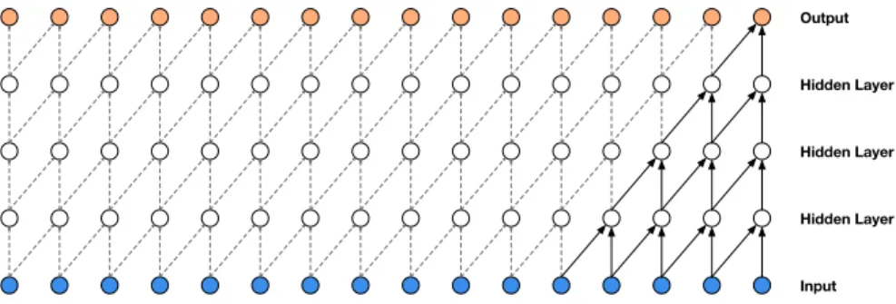
Figure 2: Visualization of a stack of causal convolutional layers.
The main ingredient of WaveNet are causal convolutions. By using causal convolutions, we make sure the model cannot violate the ordering in which we model the data: the prediction p(xt+1|x1, ..., xt)emitted by the model at timesteptcannot depend on any of the future timesteps
xt+1, xt+2, . . . , xT as shown in Fig. 2. For images, the equivalent of a causal convolution is a
masked convolution (van den Oord et al., 2016a) which can be implemented by constructing a mask tensor and doing an elementwise multiplication of this mask with the convolution kernel before ap-plying it. For 1-D data such as audio one can more easily implement this by shifting the output of a normal convolution by a few timesteps.
Because models with causal convolutions do not have recurrent connections, they are typically faster to train than RNNs, especially when applied to very long sequences. One of the problems of causal convolutions is that they require many layers, or large filters to increase the receptive field. For example, in Fig. 2 the receptive field is only 5 (= #layers + filter length - 1). In this paper we use dilated convolutions to increase the receptive field by orders of magnitude, without greatly increasing computational cost.
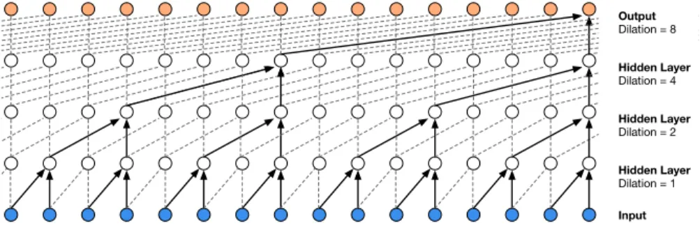
A dilated convolution (also called `a trous, or convolution with holes) is a convolution where the filter is applied over an area larger than its length by skipping input values with a certain step. It is equivalent to a convolution with a larger filter derived from the original filter by dilating it with zeros, but is significantly more efficient. A dilated convolution effectively allows the network to operate on a coarser scale than with a normal convolution. This is similar to pooling or strided convolutions, but here the output has the same size as the input. As a special case, dilated convolution with dilation
1yields the standard convolution. Fig. 3 depicts dilated causal convolutions for dilations1,2,4, and8. Dilated convolutions have previously been used in various contexts, e.g. signal processing (Holschneider et al., 1989; Dutilleux, 1989), and image segmentation (Chen et al., 2015; Yu & Koltun, 2016).
Input Hidden Layer
Dilation = 1
Hidden Layer
Dilation = 2
Hidden Layer
Dilation = 4
Output
Dilation = 8
Figure 3: Visualization of a stack ofdilatedcausal convolutional layers.
Stacked dilated convolutions enable networks to have very large receptive fields with just a few lay-ers, while preserving the input resolution throughout the network as well as computational efficiency. In this paper, the dilation is doubled for every layer up to a limit and then repeated: e.g.
1,2,4, . . . ,512,1,2,4, . . . ,512,1,2,4, . . . ,512.
The intuition behind this configuration is two-fold. First, exponentially increasing the dilation factor results in exponential receptive field growth with depth (Yu & Koltun, 2016). For example each
1,2,4, . . . ,512block has receptive field of size1024, and can be seen as a more efficient and dis-criminative (non-linear) counterpart of a1×1024convolution. Second, stacking these blocks further increases the model capacity and the receptive field size.
2.2 SOFTMAX DISTRIBUTIONS
One approach to modeling the conditional distributions p(xt|x1, . . . , xt−1)over the individual audio samples would be to use a mixture model such as a mixture density network (Bishop, 1994) or mixture of conditional Gaussian scale mixtures (MCGSM) (Theis & Bethge, 2015). However, van den Oord et al. (2016a) showed that a softmax distribution tends to work better, even when the data is implicitly continuous (as is the case for image pixel intensities or audio sample values). One of the reasons is that a categorical distribution is more flexible and can more easily model arbitrary distributions because it makes no assumptions about their shape.
Because raw audio is typically stored as a sequence of 16-bit integer values (one per timestep), a softmax layer would need to output 65,536 probabilities per timestep to model all possible values. To make this more tractable, we first apply aµ-law companding transformation (ITU-T, 1988) to the data, and then quantize it to 256 possible values:
f(xt) = sign(xt)
where−1 < xt < 1andµ = 255. This non-linear quantization produces a significantly better
reconstruction than a simple linear quantization scheme. Especially for speech, we found that the reconstructed signal after quantization sounded very similar to the original.
2.3 GATED ACTIVATION UNITS
We use the same gated activation unit as used in the gated PixelCNN (van den Oord et al., 2016b):
z= tanh (Wf,k∗x)⊙σ(Wg,k∗x), (2)
where∗denotes a convolution operator,⊙denotes an element-wise multiplication operator,σ(·)is a sigmoid function, kis the layer index, f andg denote filter and gate, respectively, andW is a learnable convolution filter. In our initial experiments, we observed that this non-linearity worked significantly better than the rectified linear activation function (Nair & Hinton, 2010) for modeling audio signals.
2.4 RESIDUAL AND SKIP CONNECTIONS
1×1 ReLU ReLU
1×1
Dilated Conv
tanh × +
σ
1×1
+ Softmax
Residual
Skip-connections
k Layers
Output
Causal Conv
Input
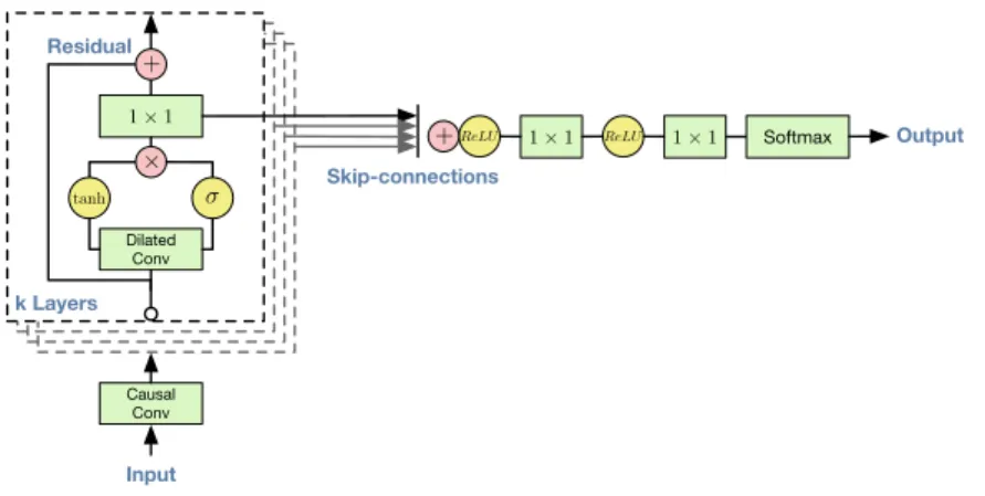
Figure 4: Overview of the residual block and the entire architecture.
Both residual (He et al., 2015) and parameterised skip connections are used throughout the network, to speed up convergence and enable training of much deeper models. In Fig. 4 we show a residual block of our model, which is stacked many times in the network.
2.5 CONDITIONALWAVENETS
Given an additional inputh, WaveNets can model the conditional distributionp(x|h)of the audio given this input. Eq. (1) now becomes
p(x|h) = T Y
t=1
p(xt|x1, . . . , xt−1,h). (3)
By conditioning the model on other input variables, we can guide WaveNet’s generation to produce audio with the required characteristics. For example, in a multi-speaker setting we can choose the speaker by feeding the speaker identity to the model as an extra input. Similarly, for TTS we need to feed information about the text as an extra input.
We condition the model on other inputs in two different ways: global conditioning and local condi-tioning. Global conditioning is characterised by a single latent representationhthat influences the output distribution across all timesteps, e.g. a speaker embedding in a TTS model. The activation function from Eq. (2) now becomes:
z= tanh Wf,k∗x+Vf,kT h
⊙σ Wg,k∗x+Vg,kT h
whereV∗,kis a learnable linear projection, and the vectorV∗T,khis broadcast over the time
dimen-sion.
For local conditioning we have a second timeseriesht, possibly with a lower sampling frequency
than the audio signal, e.g. linguistic features in a TTS model. We first transform this time series using a transposed convolutional network (learned upsampling) that maps it to a new time series y=f(h)with the same resolution as the audio signal, which is then used in the activation unit as follows:
z= tanh (Wf,k∗x+Vf,k∗y)⊙σ(Wg,k∗x+Vg,k∗y),
whereVf,k∗yis now a1×1convolution. As an alternative to the transposed convolutional network,
it is also possible to useVf,k∗hand repeat these values across time. We saw that this worked slightly
worse in our experiments.
2.6 CONTEXT STACKS
We have already mentioned several different ways to increase the receptive field size of a WaveNet: increasing the number of dilation stages, using more layers, larger filters, greater dilation factors, or a combination thereof. A complementary approach is to use a separate, smallercontextstack that processes a long part of the audio signal and locally conditions a larger WaveNet that processes only a smaller part of the audio signal (cropped at the end). One can use multiple context stacks with varying lengths and numbers of hidden units. Stacks with larger receptive fields have fewer units per layer. Context stacks can also have pooling layers to run at a lower frequency. This keeps the computational requirements at a reasonable level and is consistent with the intuition that less capacity is required to model temporal correlations at longer timescales.
3
E
XPERIMENTSTo measure WaveNet’s audio modelling performance, we evaluate it on three different tasks: multi-speaker speech generation (not conditioned on text), TTS, and music audio modelling. We provide samples drawn from WaveNet for these experiments on the accompanying webpage:
https://www.deepmind.com/blog/wavenet-generative-model-raw-audio/.
3.1 MULTI-SPEAKERSPEECHGENERATION
For the first experiment we looked at free-form speech generation (not conditioned on text). We used the English multi-speaker corpus from CSTR voice cloning toolkit (VCTK) (Yamagishi, 2012) and conditioned WaveNet only on the speaker. The conditioning was applied by feeding the speaker ID to the model in the form of a one-hot vector. The dataset consisted of 44 hours of data from 109 different speakers.
Because the model is not conditioned on text, it generates non-existent but human language-like words in a smooth way with realistic sounding intonations. This is similar to generative models of language or images, where samples look realistic at first glance, but are clearly unnatural upon closer inspection. The lack of long range coherence is partly due to the limited size of the model’s receptive field (about 300 milliseconds), which means it can only remember the last 2–3 phonemes it produced.
A single WaveNet was able to model speech from any of the speakers by conditioning it on a one-hot encoding of a speaker. This confirms that it is powerful enough to capture the characteristics of all 109 speakers from the dataset in a single model. We observed that adding speakers resulted in better validation set performance compared to training solely on a single speaker. This suggests that WaveNet’s internal representation was shared among multiple speakers.
3.2 TEXT-TO-SPEECH
For the second experiment we looked at TTS. We used the same single-speaker speech databases from which Google’s North American English and Mandarin Chinese TTS systems are built. The North American English dataset contains 24.6 hours of speech data, and the Mandarin Chinese dataset contains 34.8 hours; both were spoken by professional female speakers.
WaveNets for the TTS task were locally conditioned on linguistic features which were derived from input texts. We also trained WaveNets conditioned on the logarithmic fundamental frequency (logF0) values in addition to the linguistic features. External models predictinglogF0values and phone durations from linguistic features were also trained for each language. The receptive field size of the WaveNets was 240 milliseconds. As example-based and model-based speech synthesis base-lines, hidden Markov model (HMM)-driven unit selection concatenative (Gonzalvo et al., 2016) and long short-term memory recurrent neural network (LSTM-RNN)-based statistical parametric (Zen et al., 2016) speech synthesizers were built. Since the same datasets and linguistic features were used to train both the baselines and WaveNets, these speech synthesizers could be fairly compared.
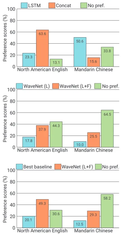
To evaluate the performance of WaveNets for the TTS task, subjective paired comparison tests and mean opinion score (MOS) tests were conducted. In the paired comparison tests, after listening to each pair of samples, the subjects were asked to choose which they preferred, though they could choose “neutral” if they did not have any preference. In the MOS tests, after listening to each stimulus, the subjects were asked to rate the naturalness of the stimulus in a five-point Likert scale score (1: Bad, 2: Poor, 3: Fair, 4: Good, 5: Excellent). Please refer to Appendix B for details.
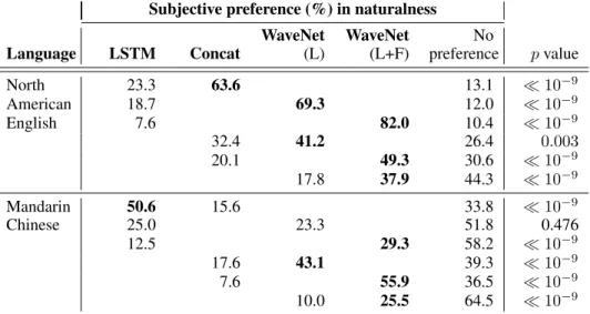
Fig. 5 shows a selection of the subjective paired comparison test results (see Appendix B for the complete table). It can be seen from the results that WaveNet outperformed the baseline statisti-cal parametric and concatenative speech synthesizers in both languages. We found that WaveNet conditioned on linguistic features could synthesize speech samples with natural segmental quality but sometimes it had unnatural prosody by stressing wrong words in a sentence. This could be due to the long-term dependency ofF0 contours: the size of the receptive field of the WaveNet, 240 milliseconds, was not long enough to capture such long-term dependency. WaveNet conditioned on both linguistic features andF0values did not have this problem: the externalF0prediction model runs at a lower frequency (200 Hz) so it can learn long-range dependencies that exist inF0contours.
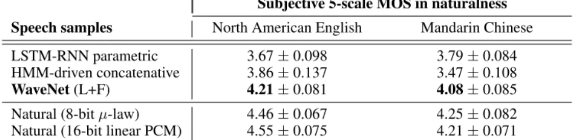
Table 1 show the MOS test results. It can be seen from the table that WaveNets achieved 5-scale MOSs in naturalness above 4.0, which were significantly better than those from the baseline systems. They were the highest ever reported MOS values with these training datasets and test sentences. The gap in the MOSs from the best synthetic speech to the natural ones decreased from 0.69 to 0.34 (51%) in US English and 0.42 to 0.13 (69%) in Mandarin Chinese.
Subjective 5-scale MOS in naturalness
Speech samples North American English Mandarin Chinese
LSTM-RNN parametric 3.67±0.098 3.79±0.084 HMM-driven concatenative 3.86±0.137 3.47±0.108 WaveNet(L+F) 4.21±0.081 4.08±0.085
Natural (8-bitµ-law) 4.46±0.067 4.25±0.082 Natural (16-bit linear PCM) 4.55±0.075 4.21±0.071
Table 1: Subjective 5-scale mean opinion scores of speech samples from LSTM-RNN-based sta-tistical parametric, HMM-driven unit selection concatenative, and proposed WaveNet-based speech synthesizers, 8-bitµ-law encoded natural speech, and 16-bit linear pulse-code modulation (PCM) natural speech. WaveNet improved the previous state of the art significantly, reducing the gap be-tween natural speech and best previous model by more than 50%.
3.3 MUSIC
0 20 40 60 80
100 LSTM Concat No pref.
Mandarin Chinese North American English
P re fe re n c e s c o re s ( % ) 23.3 13.1 63.6 50.6 33.8 15.6 0 20 40 60 80
100 WaveNet (L) WaveNet (L+F) No pref.
Mandarin Chinese North American English
P re fe re n c e s c o re s ( % ) 17.8 44.3 37.9 10.0 64.5 25.5 0 20 40 60 80
100 Best baseline WaveNet (L+F) No pref.
Mandarin Chinese North American English
P re fe re n c e s c o re s ( % ) 20.1 49.3 30.6 12.5 29.3 58.2
• the MagnaTagATune dataset (Law & Von Ahn, 2009), which consists of about 200 hours of music audio. Each 29-second clip is annotated with tags from a set of 188, which describe the genre, instrumentation, tempo, volume and mood of the music.
• the YouTube piano dataset, which consists of about 60 hours of solo piano music obtained from YouTube videos. Because it is constrained to a single instrument, it is considerably easier to model.
Although it is difficult to quantitatively evaluate these models, a subjective evaluation is possible by listening to the samples they produce. We found that enlarging the receptive field was crucial to ob-tain samples that sounded musical. Even with a receptive field of several seconds, the models did not enforce long-range consistency which resulted in second-to-second variations in genre, instrumen-tation, volume and sound quality. Nevertheless, the samples were often harmonic and aesthetically pleasing, even when produced by unconditional models.
Of particular interest are conditional music models, which can generate music given a set of tags specifying e.g. genre or instruments. Similarly to conditional speech models, we insert biases that depend on a binary vector representation of the tags associated with each training clip. This makes it possible to control various aspects of the output of the model when sampling, by feeding in a binary vector that encodes the desired properties of the samples. We have trained such models on the MagnaTagATune dataset; although the tag data bundled with the dataset was relatively noisy and had many omissions, after cleaning it up by merging similar tags and removing those with too few associated clips, we found this approach to work reasonably well.
3.4 SPEECHRECOGNITION
Although WaveNet was designed as a generative model, it can straightforwardly be adapted to dis-criminative audio tasks such as speech recognition.
Traditionally, speech recognition research has largely focused on using log mel-filterbank energies or mel-frequency cepstral coefficients (MFCCs), but has been moving to raw audio recently (Palaz et al., 2013; T¨uske et al., 2014; Hoshen et al., 2015; Sainath et al., 2015). Recurrent neural networks such as LSTM-RNNs (Hochreiter & Schmidhuber, 1997) have been a key component in these new speech classification pipelines, because they allow for building models with long range contexts. With WaveNets we have shown that layers of dilated convolutions allow the receptive field to grow longer in a much cheaper way than using LSTM units.
As a last experiment we looked at speech recognition with WaveNets on the TIMIT (Garofolo et al., 1993) dataset. For this task we added a mean-pooling layer after the dilated convolutions that ag-gregated the activations to coarser frames spanning 10 milliseconds (160×downsampling). The pooling layer was followed by a few non-causal convolutions. We trained WaveNet with two loss terms, one to predict the next sample and one to classify the frame, the model generalized better than with a single loss and achieved18.8 PER on the test set, which is to our knowledge the best score obtained from a model trained directly on raw audio on TIMIT.
4
C
ONCLUSIONThis paper has presented WaveNet, a deep generative model of audio data that operates directly at the waveform level. WaveNets are autoregressive and combine causal filters with dilated convolu-tions to allow their receptive fields to grow exponentially with depth, which is important to model the long-range temporal dependencies in audio signals. We have shown how WaveNets can be con-ditioned on other inputs in a global (e.g. speaker identity) or local way (e.g. linguistic features). When applied to TTS, WaveNets produced samples that outperform the current best TTS systems in subjective naturalness. Finally, WaveNets showed very promising results when applied to music audio modeling and speech recognition.
A
CKNOWLEDGEMENTSGaffney and Steve Crossan for helping to manage the project, Faith Mackinder for help with prepar-ing the blogpost, James Besley for legal support and Demis Hassabis for managprepar-ing the project and his inputs.
R
EFERENCESAgiomyrgiannakis, Yannis. Vocaine the vocoder and applications is speech synthesis. InICASSP, pp. 4230–4234, 2015.
Bishop, Christopher M. Mixture density networks. Technical Report NCRG/94/004, Neural Com-puting Research Group, Aston University, 1994.
Chen, Liang-Chieh, Papandreou, George, Kokkinos, Iasonas, Murphy, Kevin, and Yuille, Alan L. Semantic image segmentation with deep convolutional nets and fully connected CRFs. InICLR, 2015. URLhttp://arxiv.org/abs/1412.7062.
Chiba, Tsutomu and Kajiyama, Masato. The Vowel: Its Nature and Structure. Tokyo-Kaiseikan, 1942.
Dudley, Homer. Remaking speech. The Journal of the Acoustical Society of America, 11(2):169– 177, 1939.
Dutilleux, Pierre. An implementation of the “algorithme `a trous” to compute the wavelet transform. In Combes, Jean-Michel, Grossmann, Alexander, and Tchamitchian, Philippe (eds.),Wavelets:
Time-Frequency Methods and Phase Space, pp. 298–304. Springer Berlin Heidelberg, 1989.
Fan, Yuchen, Qian, Yao, and Xie, Feng-Long, Soong Frank K. TTS synthesis with bidirectional LSTM based recurrent neural networks. InInterspeech, pp. 1964–1968, 2014.
Fant, Gunnar.Acoustic Theory of Speech Production. Mouton De Gruyter, 1970.
Garofolo, John S., Lamel, Lori F., Fisher, William M., Fiscus, Jonathon G., and Pallett, David S. DARPA TIMIT acoustic-phonetic continuous speech corpus CD-ROM. NIST speech disc 1-1.1.
NASA STI/Recon technical report, 93, 1993.
Gonzalvo, Xavi, Tazari, Siamak, Chan, Chun-an, Becker, Markus, Gutkin, Alexander, and Silen, Hanna. Recent advances in Google real-time HMM-driven unit selection synthesizer. In
Inter-speech, 2016. URLhttp://research.google.com/pubs/pub45564.html.
He, Kaiming, Zhang, Xiangyu, Ren, Shaoqing, and Sun, Jian. Deep residual learning for image recognition.CoRR, abs/1512.03385, 2015.
Hochreiter, S. and Schmidhuber, J. Long short-term memory. Neural Comput., 9(8):1735–1780, 1997.
Holschneider, Matthias, Kronland-Martinet, Richard, Morlet, Jean, and Tchamitchian, Philippe. A real-time algorithm for signal analysis with the help of the wavelet transform. In Combes, Jean-Michel, Grossmann, Alexander, and Tchamitchian, Philippe (eds.), Wavelets: Time-Frequency
Methods and Phase Space, pp. 286–297. Springer Berlin Heidelberg, 1989.
Hoshen, Yedid, Weiss, Ron J., and Wilson, Kevin W. Speech acoustic modeling from raw multi-channel waveforms. InICASSP, pp. 4624–4628. IEEE, 2015.
Hunt, Andrew J. and Black, Alan W. Unit selection in a concatenative speech synthesis system using a large speech database. InICASSP, pp. 373–376, 1996.
Imai, Satoshi and Furuichi, Chieko. Unbiased estimation of log spectrum. InEURASIP, pp. 203– 206, 1988.
Itakura, Fumitada. Line spectrum representation of linear predictor coefficients of speech signals.
The Journal of the Acoust. Society of America, 57(S1):S35–S35, 1975.
ITU-T. Recommendation G. 711.Pulse Code Modulation (PCM) of voice frequencies, 1988.
J´ozefowicz, Rafal, Vinyals, Oriol, Schuster, Mike, Shazeer, Noam, and Wu, Yonghui. Exploring the limits of language modeling.CoRR, abs/1602.02410, 2016. URLhttp://arxiv.org/abs/
1602.02410.
Juang, Biing-Hwang and Rabiner, Lawrence. Mixture autoregressive hidden Markov models for speech signals.IEEE Trans. Acoust. Speech Signal Process., pp. 1404–1413, 1985.
Kameoka, Hirokazu, Ohishi, Yasunori, Mochihashi, Daichi, and Le Roux, Jonathan. Speech anal-ysis with multi-kernel linear prediction. InSpring Conference of ASJ, pp. 499–502, 2010. (in Japanese).
Karaali, Orhan, Corrigan, Gerald, Gerson, Ira, and Massey, Noel. Text-to-speech conversion with neural networks: A recurrent TDNN approach. InEurospeech, pp. 561–564, 1997.
Kawahara, Hideki, Masuda-Katsuse, Ikuyo, and de Cheveign´e, Alain. Restructuring speech rep-resentations using a pitch-adaptive time-frequency smoothing and an instantaneous-frequency-basedf0extraction: possible role of a repetitive structure in sounds. Speech Commn., 27:187– 207, 1999.
Kawahara, Hideki, Estill, Jo, and Fujimura, Osamu. Aperiodicity extraction and control using mixed mode excitation and group delay manipulation for a high quality speech analysis, modification and synthesis system STRAIGHT. InMAVEBA, pp. 13–15, 2001.
Law, Edith and Von Ahn, Luis. Input-agreement: a new mechanism for collecting data using human computation games. InProceedings of the SIGCHI Conference on Human Factors in Computing
Systems, pp. 1197–1206. ACM, 2009.
Maia, Ranniery, Zen, Heiga, and Gales, Mark J. F. Statistical parametric speech synthesis with joint estimation of acoustic and excitation model parameters. InISCA SSW7, pp. 88–93, 2010.
Morise, Masanori, Yokomori, Fumiya, and Ozawa, Kenji. WORLD: A vocoder-based high-quality speech synthesis system for real-time applications.IEICE Trans. Inf. Syst., E99-D(7):1877–1884, 2016.
Moulines, Eric and Charpentier, Francis. Pitch synchronous waveform processing techniques for text-to-speech synthesis using diphones.Speech Commn., 9:453–467, 1990.
Muthukumar, P. and Black, Alan W. A deep learning approach to data-driven parameterizations for statistical parametric speech synthesis.arXiv:1409.8558, 2014.
Nair, Vinod and Hinton, Geoffrey E. Rectified linear units improve restricted Boltzmann machines. InICML, pp. 807–814, 2010.
Nakamura, Kazuhiro, Hashimoto, Kei, Nankaku, Yoshihiko, and Tokuda, Keiichi. Integration of spectral feature extraction and modeling for HMM-based speech synthesis. IEICE Trans. Inf.
Syst., E97-D(6):1438–1448, 2014.
Palaz, Dimitri, Collobert, Ronan, and Magimai-Doss, Mathew. Estimating phoneme class condi-tional probabilities from raw speech signal using convolucondi-tional neural networks. InInterspeech, pp. 1766–1770, 2013.
Peltonen, Sari, Gabbouj, Moncef, and Astola, Jaakko. Nonlinear filter design: methodologies and challenges. InIEEE ISPA, pp. 102–107, 2001.
Poritz, Alan B. Linear predictive hidden Markov models and the speech signal. InICASSP, pp. 1291–1294, 1982.
Rabiner, Lawrence and Juang, Biing-Hwang. Fundamentals of Speech Recognition. PrenticeHall, 1993.
Sainath, Tara N., Weiss, Ron J., Senior, Andrew, Wilson, Kevin W., and Vinyals, Oriol. Learning the speech front-end with raw waveform CLDNNs. InInterspeech, pp. 1–5, 2015.
Takaki, Shinji and Yamagishi, Junichi. A deep auto-encoder based low-dimensional feature ex-traction from FFT spectral envelopes for statistical parametric speech synthesis. InICASSP, pp. 5535–5539, 2016.
Takamichi, Shinnosuke, Toda, Tomoki, Black, Alan W., Neubig, Graham, Sakriani, Sakti, and Naka-mura, Satoshi. Postfilters to modify the modulation spectrum for statistical parametric speech synthesis.IEEE/ACM Trans. Audio Speech Lang. Process., 24(4):755–767, 2016.
Theis, Lucas and Bethge, Matthias. Generative image modeling using spatial LSTMs. InNIPS, pp. 1927–1935, 2015.
Toda, Tomoki and Tokuda, Keiichi. A speech parameter generation algorithm considering global variance for HMM-based speech synthesis.IEICE Trans. Inf. Syst., E90-D(5):816–824, 2007.
Toda, Tomoki and Tokuda, Keiichi. Statistical approach to vocal tract transfer function estimation based on factor analyzed trajectory hmm. InICASSP, pp. 3925–3928, 2008.
Tokuda, Keiichi. Speech synthesis as a statistical machine learning problem. http://www.sp.
nitech.ac.jp/˜tokuda/tokuda_asru2011_for_pdf.pdf, 2011. Invited talk given
at ASRU.
Tokuda, Keiichi and Zen, Heiga. Directly modeling speech waveforms by neural networks for statistical parametric speech synthesis. InICASSP, pp. 4215–4219, 2015.
Tokuda, Keiichi and Zen, Heiga. Directly modeling voiced and unvoiced components in speech waveforms by neural networks. InICASSP, pp. 5640–5644, 2016.
Tuerk, Christine and Robinson, Tony. Speech synthesis using artificial neural networks trained on cepstral coefficients. InProc. Eurospeech, pp. 1713–1716, 1993.
T¨uske, Zolt´an, Golik, Pavel, Schl¨uter, Ralf, and Ney, Hermann. Acoustic modeling with deep neural networks using raw time signal for LVCSR. InInterspeech, pp. 890–894, 2014.
Uria, Benigno, Murray, Iain, Renals, Steve, Valentini-Botinhao, Cassia, and Bridle, John. Modelling acoustic feature dependencies with artificial neural networks: Trajectory-RNADE. InICASSP, pp. 4465–4469, 2015.
van den Oord, A¨aron, Kalchbrenner, Nal, and Kavukcuoglu, Koray. Pixel recurrent neural networks.
arXiv preprint arXiv:1601.06759, 2016a.
van den Oord, A¨aron, Kalchbrenner, Nal, Vinyals, Oriol, Espeholt, Lasse, Graves, Alex, and Kavukcuoglu, Koray. Conditional image generation with PixelCNN decoders. CoRR, abs/1606.05328, 2016b. URLhttp://arxiv.org/abs/1606.05328.
Wu, Yi-Jian and Tokuda, Keiichi. Minimum generation error training with direct log spectral distor-tion on LSPs for HMM-based speech synthesis. InInterspeech, pp. 577–580, 2008.
Yamagishi, Junichi. English multi-speaker corpus for CSTR voice cloning toolkit, 2012. URL
http://homepages.inf.ed.ac.uk/jyamagis/page3/page58/page58.html.
Yoshimura, Takayoshi. Simultaneous modeling of phonetic and prosodic parameters, and
char-acteristic conversion for HMM-based text-to-speech systems. PhD thesis, Nagoya Institute of
Technology, 2002.
Yu, Fisher and Koltun, Vladlen. Multi-scale context aggregation by dilated convolutions. InICLR, 2016. URLhttp://arxiv.org/abs/1511.07122.
Speech Speech
Text Text
Feature prediction
Vocoder synthesis
Text analysis Vocoder
analysis
Text analysis
Model training
l o
l Λ
ˆ Acoustic
model
ˆ o
Training Synthesis
Figure 6: Outline of statistical parametric speech synthesis.
Zen, Heiga, Tokuda, Keiichi, and Kitamura, Tadashi. Reformulating the HMM as a trajectory model by imposing explicit relationships between static and dynamic features. Comput. Speech Lang., 21(1):153–173, 2007.
Zen, Heiga, Tokuda, Keiichi, and Black, Alan W. Statistical parametric speech synthesis. Speech
Commn., 51(11):1039–1064, 2009.
Zen, Heiga, Senior, Andrew, and Schuster, Mike. Statistical parametric speech synthesis using deep neural networks. InProc. ICASSP, pp. 7962–7966, 2013.
Zen, Heiga, Agiomyrgiannakis, Yannis, Egberts, Niels, Henderson, Fergus, and Szczepaniak, Prze-mysław. Fast, compact, and high quality LSTM-RNN based statistical parametric speech synthe-sizers for mobile devices. InInterspeech, 2016. URLhttps://arxiv.org/abs/1606.
06061.
A
T
EXT-
TO-S
PEECHB
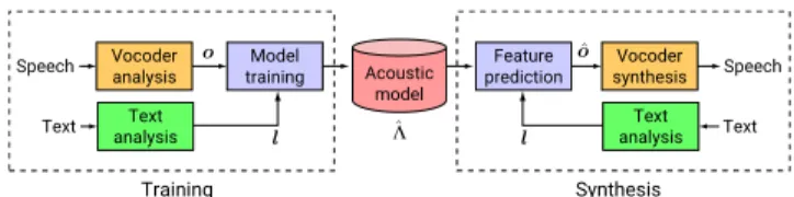
ACKGROUNDThe goal of TTS synthesis is to render naturally sounding speech signals given a text to be syn-thesized. Human speech production process first translates a text (or concept) into movements of muscles associated with articulators and speech production-related organs. Then using air-flow from lung, vocal source excitation signals, which contain both periodic (by vocal cord vibration) and aperiodic (by turbulent noise) components, are generated. By filtering the vocal source excitation signals by time-varying vocal tract transfer functions controlled by the articulators, their frequency characteristics are modulated. Finally, the generated speech signals are emitted. The aim of TTS is to mimic this process by computers in some way.
TTS can be viewed as a sequence-to-sequence mapping problem; from a sequence of discrete sym-bols (text) to a real-valued time series (speech signals). A typical TTS pipeline has two parts; 1) text analysis and 2) speech synthesis. The text analysis part typically includes a number of natural language processing (NLP) steps, such as sentence segmentation, word segmentation, text normal-ization, part-of-speech (POS) tagging, and grapheme-to-phoneme (G2P) conversion. It takes a word sequence as input and outputs a phoneme sequence with a variety of linguistic contexts. The speech synthesis part takes the context-dependent phoneme sequence as its input and outputs a synthesized speech waveform. This part typically includes prosody prediction and speech waveform generation.
There are two main approaches to realize the speech synthesis part; non-parametric, example-based approach known as concatenative speech synthesis (Moulines & Charpentier, 1990; Sagisaka et al., 1992; Hunt & Black, 1996), and parametric, model-based approach known as statistical parametric speech synthesis (Yoshimura, 2002; Zen et al., 2009). The concatenative approach builds up the utterance from units of recorded speech, whereas the statistical parametric approach uses a gener-ative model to synthesize the speech. The statistical parametric approach first extracts a sequence of vocoder parameters (Dudley, 1939)o= {o1, . . . ,oN}from speech signalsx= {x1, . . . , xT}
and linguistic featureslfrom the text W, whereN andT correspond to the numbers of vocoder parameter vectors and speech signals. Typically a vocoder parameter vectoronis extracted at
as
ˆ
Λ = arg max
Λ
p(o|l,Λ), (4)
whereΛdenotes the set of parameters of the generative model. At the synthesis stage, the most probable vocoder parameters are generated given linguistic features extracted from a text to be syn-thesized as
ˆ
o= arg max o
p(o|l,Λ)ˆ . (5)
Then a speech waveform is reconstructed fromoˆ using a vocoder. The statistical parametric ap-proach offers various advantages over the concatenative one such as small footprint and flexibility to change its voice characteristics. However, its subjective naturalness is often significantly worse than that of the concatenative approach; synthesized speech often sounds muffled and has artifacts. Zen et al. (2009) reported three major factors that can degrade the subjective naturalness; quality of vocoders, accuracy of generative models, and effect of oversmoothing. The first factor causes the artifacts and the second and third factors lead to the muffleness in the synthesized speech. There have been a number of attempts to address these issues individually, such as developing high-quality vocoders (Kawahara et al., 1999; Agiomyrgiannakis, 2015; Morise et al., 2016), improving the ac-curacy of generative models (Zen et al., 2007; 2013; Fan et al., 2014; Uria et al., 2015), and compen-sating the oversmoothing effect (Toda & Tokuda, 2007; Takamichi et al., 2016). Zen et al. (2016) showed that state-of-the-art statistical parametric speech syntheziers matched state-of-the-art con-catenative ones in some languages. However, its vocoded sound quality is still a major issue.
Extracting vocoder parameters can be viewed as estimation of a generative model parameters given speech signals (Itakura & Saito, 1970; Imai & Furuichi, 1988). For example, linear predictive anal-ysis (Itakura & Saito, 1970), which has been used in speech coding, assumes that the generative model of speech signals is a linear auto-regressive (AR) zero-mean Gaussian process;
xt= P X
p=1
apxt−p+ǫt (6)
ǫt∼ N(0, G2) (7)
whereapis ap-th order linear predictive coefficient (LPC) andG2is a variance of modeling error.
These parameters are estimated based on the maximum likelihood (ML) criterion. In this sense, the training part of the statistical parametric approach can be viewed as a two-step optimization and sub-optimal: extract vocoder parameters by fitting a generative model of speech signals then model trajectories of the extracted vocoder parameters by a separate generative model for time series (Tokuda, 2011). There have been attempts to integrate these two steps into a single one (Toda & Tokuda, 2008; Wu & Tokuda, 2008; Maia et al., 2010; Nakamura et al., 2014; Muthukumar & Black, 2014; Tokuda & Zen, 2015; 2016; Takaki & Yamagishi, 2016). For example, Tokuda & Zen (2016) integrated non-stationary, nonzero-mean Gaussian process generative model of speech signals and LSTM-RNN-based sequence generative model to a single one and jointly optimized them by back-propagation. Although they showed that this model could approximate natural speech signals, its segmental naturalness was significantly worse than the non-integrated model due to over-generalization and over-estimation of noise components in speech signals.
The conventional generative models of raw audio signals have a number of assumptions which are inspired from the speech production, such as
• Use of fixed-length analysis window; They are typically based on a stationary stochas-tic process (Itakura & Saito, 1970; Imai & Furuichi, 1988; Poritz, 1982; Juang & Rabiner, 1985; Kameoka et al., 2010). To model time-varying speech signals by a stationary stochas-tic process, parameters of these generative models are estimated within a fixed-length, over-lapping and shifting analysis window (typically its length is 20 to 30 milliseconds, and shift is 5 to 10 milliseconds). However, some phones such as stops are time-limited by less than 20 milliseconds (Rabiner & Juang, 1993). Therefore, using such fixed-size analysis win-dow has limitations.
• Gaussian process assumption; The conventional generative models are based on Gaussian process (Itakura & Saito, 1970; Imai & Furuichi, 1988; Poritz, 1982; Juang & Rabiner, 1985; Kameoka et al., 2010; Tokuda & Zen, 2015; 2016). From the source-filter model of speech production (Chiba & Kajiyama, 1942; Fant, 1970) point of view, this is equivalent to assuming that a vocal source excitation signal is a sample from a Gaussian distribu-tion (Itakura & Saito, 1970; Imai & Furuichi, 1988; Poritz, 1982; Juang & Rabiner, 1985; Tokuda & Zen, 2015; Kameoka et al., 2010; Tokuda & Zen, 2016). Together with the lin-ear assumption above, it results in assuming that speech signals are normally distributed. However, distributions of real speech signals can be significantly different from Gaussian.
Although these assumptions are convenient, samples from these generative models tend to be noisy and lose important details to make these audio signals sounding natural.
WaveNet, which was described in Section 2, has none of the above-mentioned assumptions. It incorporates almost no prior knowledge about audio signals, except the choice of the receptive field andµ-law encoding of the signal. It can also be viewed as a non-linear causal filter for quantized signals. Although such non-linear filter can represent complicated signals while preserving the details, designing such filters is usually difficult (Peltonen et al., 2001). WaveNets give a way to train them from data.
B
D
ETAILS OFTTS E
XPERIMENTThe HMM-driven unit selection and WaveNet TTS systems were built from speech at 16 kHz sam-pling. Although LSTM-RNNs were trained from speech at 22.05 kHz sampling, speech at 16 kHz sampling was synthesized at runtime using a resampling functionality in the Vocaine vocoder (Agiomyrgiannakis, 2015). Both the LSTM-RNN-based statistical parametric and HMM-driven unit selection speech synthesizers were built from the speech datasets in the 16-bit linear PCM, whereas the WaveNet-based ones were trained from the same speech datasets in the 8-bitµ-law encoding.
The linguistic features include phone, syllable, word, phrase, and utterance-level features (Zen, 2006) (e.g. phone identities, syllable stress, the number of syllables in a word, and position of the current syllable in a phrase) with additional frame position and phone duration features (Zen et al., 2013). These features were derived and associated with speech every 5 milliseconds by phone-level forced alignment at the training stage. We used LSTM-RNN-based phone duration and autoregres-sive CNN-basedlogF0prediction models. They were trained so as to minimize the mean squared errors (MSE). It is important to note that no post-processing was applied to the audio signals gener-ated from the WaveNets.
Subjective preference (%) in naturalness
WaveNet WaveNet No
Language LSTM Concat (L) (L+F) preference pvalue
North 23.3 63.6 13.1 ≪10−9
American 18.7 69.3 12.0 ≪10−9
English 7.6 82.0 10.4 ≪10−9
32.4 41.2 26.4 0.003
20.1 49.3 30.6 ≪10−9
17.8 37.9 44.3 ≪10−9
Mandarin 50.6 15.6 33.8 ≪10−9
Chinese 25.0 23.3 51.8 0.476
12.5 29.3 58.2 ≪10−9
17.6 43.1 39.3 ≪10−9
7.6 55.9 36.5 ≪10−9
10.0 25.5 64.5 ≪10−9