Article
A Stackelberg Game Approach in an Integrated
Inventory Model with Carbon-Emission and Setup
Cost Reduction
Biswajit Sarkar1, Sharmila Saren2, Mitali Sarkar1and Yong Won Seo3,*
1 Department of Industrial & Management Engineering, Hanyang University, Ansan Gyeonggi-do 15588,
Korea; [email protected] (B.S.); [email protected] (M.S.)
2 Department of Applied Mathematics with Oceanology and Computer Programming, Vidyasagar University,
Midnapore 721 102, India; [email protected]
3 Department of Business Administration, College of Business and Economics, Chung-Ang University,
Dongjak, Seoul 06974, Korea
* Correspondence: [email protected]; Tel.: +82-10-6858-1683; +82-2-820-5580
Academic Editor: Marc A. Rosen
Received: 5 September 2016; Accepted: 22 November 2016; Published: 2 December 2016
Abstract:This paper formulates an integrated inventory model that allows Stackelberg game policy for optimizing joint total cost of a vendor and buyer system. After receiving the lot, the buyer commences an inspection process to determine the defective items. All defective items the buyer sends to vendor during the receiving of the next lot. Due to increasing number of shipments fixed and variable transportation, as well as carbon emissions, are considered, which makes the model sustainable integrated model forever. To reduce the setup cost for the vendor, a discrete setup reduction is considered for maximization more profit. The players of the integrated model are with unequal power (as leader and follower) and the Stackelberg game strategy is utilized to solve this model for obtaining global optimum solution over the finite planning horizon. An illustrative numerical example is given to understand this model clearly.
Keywords:integrated-inventory model; stackelberg approach; setup cost reduction; transportation cost; carbon emission reduction
1. Introduction
Generally, an integrated-production-inventory model defines the vendor-buyer or retailer-customer model. In that type of model, usually a vendor produces an item in a production batch line and the produced finished goods are transferred to several buyers. In spite of that, retailer’s production cycle time is measured as an integer multiple of the function of consumer’s ordering time. Many research articles highlighted various integrated vendor-buyer models with several key parameters. Chang et al. [1] discussed an integrated vendor-buyer inventory system under trade-credit policies. Demand is measured as the diminishing function of retail-price. Additionally, they surveyed an iterative algorithm to figure out the optimal retail-price, number of buyer’s ordering amount, and numbers of deliveries per production run. Yang [2] extended previous research models considering an integrated-inventory model with lead time crashing cost. Hoque [3] analyzed a vendor-buyer integrated-production model, where lead time follows a normal distribution along with setup time of a machine, maximum boundary on capacity of shipping vehicle, cost of transportation, and batch time are also inserted in his model. Jha and Shanker [4] established an integrated inventory model with transportation for a single-vendor and multi-buyer. It is observed that the vendor produces and deliveries products to buyers in distinct locations by similar capability of some vehicles. The external demands of buyers are taken to be independent and follows a normal distribution. Lead time of
buyers without transportation time are reduced by an added crashing cost. Most of the above mentioned research articles related to the integrated-inventory model are formed with the assumption that all produced items are absolutely perfect. There are no defective items during production system. Sarkar et al. [5] expanded former integrated-inventory models by including the concept of imperfect production. An inspection policy is given to examine defective items and also provides delay-in-payments in their model. In their model, non-defective item follows a binomial distribution and lead time demand follows a mixture of normal distribution. By highlighting the trade-credit policy, Ouyang et al. [6] derived an integrated-inventory model with a capacity constraint and a permissible delay-payment system. An unit production cost is calculated as the function of rate of production. Sarkar et al. [7] analyzed a continuous review inventory model on the basis of probability distribution of lead time demand. Some investment function is applied to improve the process quality. They presented two models, one with normal distributed lead time demand and another with an unknown distributed lead time demand. Sarkar [8] discovered a vendor-buyer model by considering three steps of inspection process before vendor’s consignment. Ahmad et al. [9] formulated an integrated-inventory model which includes single-supplier, single-manufacturer, and single-retailer. In addition, imperfect production process is also considered in their model. Fauza et al. [10] provided a single-vendor and multiple buyers (SVMB) model to obtain the food inventory policy. They developed a kinetic model, which is utilized to present the quality degradation of the raw material at the vendor. In literature, there are several integrated inventory models, but no one of the above mentioned authors considered unequal power of player in the integrated model. Every model is considered to have equal power of the players. However, if the players are with unequal power then only game strategy (using leader-follower policy) can be used those models.
the retailers. Wang et al. [17] addressed a product family architecture (PFA) planning and supply chain configuration as a Stackelberg game approach. They presented the PFA decision making as an upper-level optimization problem. On the other side, the lower-level optimization problem deals with the supply chain decisions. Though there are several models considering Stackelberg game policy, but no one considered this strategy for integrated inventory model for unequal lot size within single-setup-multi-delivery policy. This research gap is fulfilled by the proposed research model.
Setup cost plays an important role in today’s advanced manufacturing companies for shipment of products on time. Setup process is not measured as a value adding constraint. Setup cost need to be discussed at the time of enhancing productivity, minimizing waste, enlarging resource utilization, and satisfy deadlines. To minimize capital investment function, manufacturer are required to reduce setup cost. Researchers made various inventory models with this concept of setup cost reduction. Denizel et al. [18] studied a dynamic lot size model in which setup costs can be reduced by several amounts depending upon the level of raw-materials. They also derived a shortest path problem for these level of raw-materials. Diaby [19] established a comprehensive model to reduce both setup time and setup cost. He also added that setup times can be reduced by contributing appropriate amounts of many resources like equipment, tooling, etc. He determined how much to cut setup time for every product and how much of each good to manufacture to minimize total cost. Nyea et al. [20] developed some inventory models to forecast optimal setup times, or optimal investment in setup reduction. In their paper, a new model based on queuing theory was formed to estimate work-in-process (WIP) levels. Freimer et al. [21] established two types of process improvements which are (i) setup costs reduction; and (ii) improvement in quality of the process. Huang et al. [22] considered setup cost reduction policy by assuming an added investment. In their paper, demand of lead time is taken to be as compound poisson distribution. Annadurai and Uthayakumar [23] analyzed a mixture-inventory model with the assumptions of setup cost reduction, backorders, and lost sales. They considered that an arrival order batch may hold some defective items. Both normally distributed demand and distribution free lead time demand are developed in their model. Sarkar and Majumder [24] discussed an integrated vendor–buyer supply chain model for setup cost reduction. In their paper, two types of models are developed. In the first model, lead time demand follows a normal distribution while their second model considers the distribution free approach for the lead time demand. Sarkar and Moon [25] extended previous models by involving the concept of quality improvement, reorder point, and also lead time in which backorder rate has a great impact. They also assumed production process as imperfect. Sarkar et al. [26] included the concept of setup cost reduction along with quality improvement. The same distribution free approaches with known mean and standard deviation are discussed in their model. Allahverdi [27] obtained independently addressed problems based on performance observers, shop, and setup times/costs environments. By providing the concept that setup cost is a logarithmic function of capital investment, Priyan and Uthayakumar [28] represented an economic manufacturing quantity (EMQ) model for imperfect production process. They assumed three types of continuous probabilistic defective function. Sarkar et al. [29] produced the impact of setup cost reduction in a deteriorated two-echelon supply chain model with deterioration. Quality improvement technique is added to their model. Sarkar et al. [30] formulated a deteriorated two-echelon supply chain model where setup cost is taken to be as variable. In this case, setup cost is directly proportional to reliability. On the other hand, the deterioration rate is taken to be as inversely proportional to reliability. There are several models in the literature considering continuous investment function for reducing setup cost, but only a single model Huang et al. [22], they only considered the realistic case. The proposed model also follows the same direction of discrete investment for reducing setup cost.
determine potential benefits, increase customer service-level by improved efficiencies, and minimize lead-time variability. Hill and Galbreth [32] proposed a single-warehouse multi-retailer supply chain model, which incurs transportation discount cost functions. Kang and Kim [33] surveyed a two-level supply chain model, where a supplier provides a set of retailers and derives a production plan for every retailer by applying the data on demands of end consumers. Transportation costs are included in their model for shipment of finished products. Deliveries are fulfilled through the same capability vehicles to several retailers in a one-time trip. Chan and Zhang [34] determined a collaborative transportation management model with a simulation approach, which is utilized to (a) analyze profits of CTM; (b) describe view-point of carrier’s flexibility; and also (c) examine delivery speed ability. Lee and Fu [35] proposed a producer-buyer supply chain model in which delivery or transportation cost is added and adjusted as a power function. Shu et al. [36] observed an integrated-production-delivery lot size model with stochastic delivery time and transportation cost, which is the function of delivery quantity. Krishnakumari [37] observed a multi-period inventory cum transportation problem (MPICTP) with single-product, single-stage for multiple suppliers and multiple destinations. In this direction of research, transportation costs along with piecewise constant setup cost are described in Pazhani et al. [38]. They developed a mixed integer nonlinear programming model to observe the optimal inventory policy for the several stages in supply chain. They assumed some vehicles of several capabilities to shipment of materials. The integrated inventory model with discrete setup cost reduction and fixed as well as variable transportation is not considered yet by any researchers.
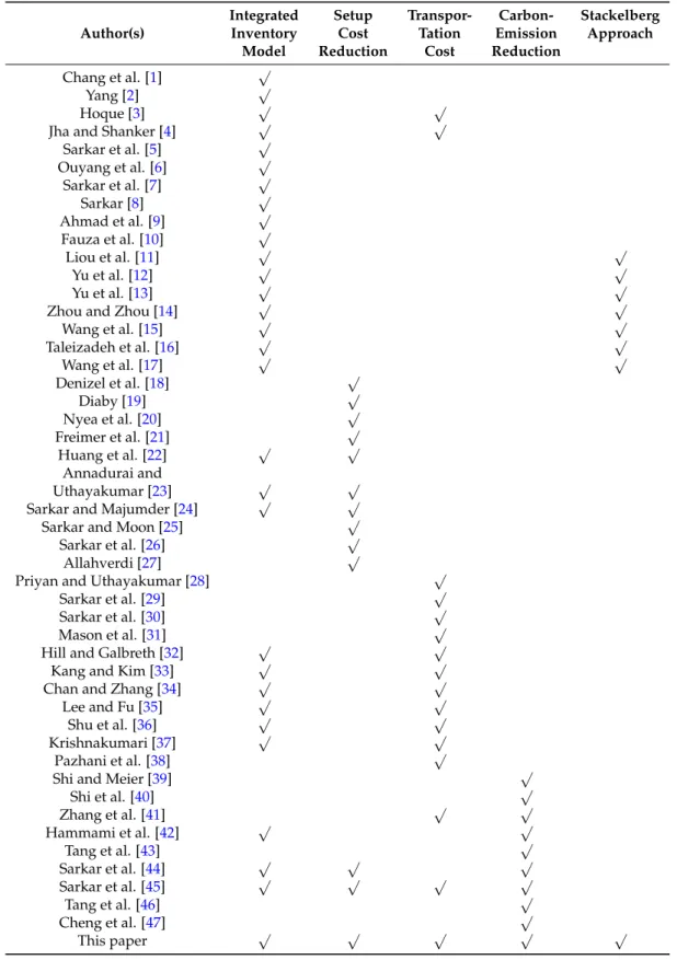
For reducing carbon-emission, production companies can monitor and enhance the emission performance of their products during their life-cycle stages. The carbon-emission assessment provides a possible mechanism to serve companies with some emission reduction. During production process, manufacturer should formulate low carbon system. There are several research papers, in which carbon-emission reduction is described briefly. To reduce global warming and carbon-emission from earth, Shi and Meier [39] presented a hybrid carbon-emission model to meet up increasing necessities of practical low-carbon matters in manufacturing systems. Shi et al. [40] described a carbon-emission reduction potential model for technology disruption and structural allowance in cement factory. They determined energy consumption and also derived the effects and trends of technological advancement. Zhang et al. [41] generated a both split and traffic assignment model, which assumed the low-carbon constraints. Their model analyzed in particular two hypothetical examine networks. Hammami et al. [42] deduced a multi-echelon supply chain model with different outside suppliers, several manufacturing facilities, distinct distribution centers, and reducing carbon-emission. Tang et al. [43] presented a periodic inventory review system by reducing carbon-emission with minimum shipment frequency. Sarkar et al. [44] produced a vendor-buyer system by assuming setup cost reduction technique, carbon-emission reduction, and inspection policy. Sarkar et al. [45] discussed a three-echelon supply chain model in which both fixed and variable transportation costs along with carbon-emission costs are included. Tang et al. [46] described a sustainable supply chain (SSC) network in which consumer environmental behaviors (CEBs) are introduced by including routing, inventory, and location. Cheng et al. [47] observed a traditional inventory routing problem (IRP) with the effects of carbon-emission regulations. There is one assembly plant and a set of geographically dispersed suppliers in that traditional inventory routing problem (IRP). They assumed transportation cost as constant with some fuel consumption cost and inventory holding cost. In their model, the fuel consumption cost is calculated by distance, fuel price, and fuel consumption rate. See Table1for the contribution of various authors.
solution methodologies. Numerical examples, graphical illustrations, sensitivity analysis are given in Section5. Finally, conclusions and future remarks are given in Section6.
Table 1.Authors contribution Table.
Integrated Setup Transpor- Carbon- Stackelberg
Author(s) Inventory Cost Tation Emission Approach
Model Reduction Cost Reduction
Chang et al. [1] √
Yang [2] √
Hoque [3] √ √
Jha and Shanker [4] √ √
Sarkar et al. [5] √ Ouyang et al. [6] √ Sarkar et al. [7] √
Sarkar [8] √
Ahmad et al. [9] √ Fauza et al. [10] √
Liou et al. [11] √ √
Yu et al. [12] √ √
Yu et al. [13] √ √
Zhou and Zhou [14] √ √
Wang et al. [15] √ √
Taleizadeh et al. [16] √ √
Wang et al. [17] √ √
Denizel et al. [18] √
Diaby [19] √
Nyea et al. [20] √
Freimer et al. [21] √
Huang et al. [22] √ √
Annadurai and
Uthayakumar [23] √ √
Sarkar and Majumder [24] √ √
Sarkar and Moon [25] √
Sarkar et al. [26] √
Allahverdi [27] √
Priyan and Uthayakumar [28] √
Sarkar et al. [29] √
Sarkar et al. [30] √
Mason et al. [31] √
Hill and Galbreth [32] √ √
Kang and Kim [33] √ √
Chan and Zhang [34] √ √
Lee and Fu [35] √ √
Shu et al. [36] √ √
Krishnakumari [37] √ √
Pazhani et al. [38] √
Shi and Meier [39] √
Shi et al. [40] √
Zhang et al. [41] √ √
Hammami et al. [42] √ √
Tang et al. [43] √
Sarkar et al. [44] √ √ √
Sarkar et al. [45] √ √ √ √
Tang et al. [46] √
Cheng et al. [47] √
2. Problem Definition, Notation, and Assumptions
This section provides the problem definition with notation and assumptions.
2.1. Problem Definition
This paper fulfils the research gap within an integrated inventory model for unequal powers of players by introducing fixed and variable transportation costs and carbon emission costs to make the model sustainable forever. To reduce the setup cost of vendor a discrete investment function is utilized. When vendor sends products to buyer, he/she conducts an inspection to ensure the quality of products for saving his/her brand image. However, after inspection, the inspection process gives some defective products, those are sent to vendor when buyer receives next lot. The number of shipment becomes an important decision variable here. Due to increasing or decreasing value of shipment number transportation and carbon emission cost may vary. Therefore, fixed and variable transportation and variable carbon emission are considered. Based on single-setup-multi-delivery (SSMD), those products are transported from vendor to buyer, but every time equal delivery lot is not possible always. Therefore, an increasing ratio of lot size is introduced to save more holding lost for reducing total cost of the system. As players of the integrated model are with unequal power, thus Stackelberg game policy is used to solve the model. The aim is to reduce total cost for making the integrated model sustainable forever.
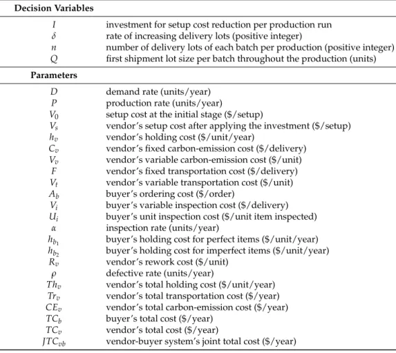
2.2. Notation
This paper considers the following some notation in Table2.
Table 2.Notation for decision variables and parameters.
Decision Variables
I investment for setup cost reduction per production run δ rate of increasing delivery lots (positive integer)
n number of delivery lots of each batch per production (positive integer) Q first shipment lot size per batch throughout the production (units)
Parameters
D demand rate (units/year) P production rate (units/year)
V0 setup cost at the initial stage ($/setup)
Vs vendor’s setup cost after applying the investment ($/setup)
hv vendor’s holding cost ($/unit/year)
Cv vendor’s fixed carbon-emission cost ($/delivery)
Vv vendor’s variable carbon-emission cost ($/unit)
F vendor’s fixed transportation cost ($/delivery) Vt vendor’s variable transportation cost ($/unit)
Ab buyer’s ordering cost ($/order)
Vi buyer’s variable inspection cost ($/delivery)
Ui buyer’s unit inspection cost ($/unit item inspected)
α inspection rate (units/year)
hb1 buyer’s holding cost for perfect items ($/unit/year) hb2 buyer’s holding cost for imperfect items ($/unit/year) Rv vendor’s rework cost ($/unit)
ρ defective rate (units/year)
Thv vendor’s total holding cost ($/unit/year)
Trv vendor’s total transportation cost ($/year)
CEv vendor’s total carbon-emission cost ($/year)
TCb buyer’s total cost ($/year)
TCv vendor’s total cost ($/year)
2.3. Assumptions
This paper makes its considerations on the basis of the following assumptions.
(1) An integrated inventory model is considered with single-buyer and single-vendor for single-type of items. To reduce setup cost, some discrete investmentIis considered. Therefore, the expression of new setup cost becomesVs(I) =V0e−κI, whereκis a known parameter. In the above equation, it is found that as the investment will be higher, the corresponding setup cost will be smaller. On the basis of such investment function, setup cost for every production run will be lower. For any business operations, the setup cost should be controlled by using this type of investment function. For instance, see Sarkar et al. [7], Huang et al. [22], Sarkar and Majumder [24], Sarkar and Moon [25], Sarkar et al. [26]. The investment decisions will effect on the setup cost and setup cost is a major cost of the production system. Therefore, the investment decision effect the whole system.
(2) Vendor transports delivery lots in a dissimilar size. Each shipment lots increases at a rateδ. The main rationale of such assumption is to reduce the holding cost of vendor. As higher holding cost has a huge impact on the total cost. Therefore, to control the holding cost, the vendor sends delivery lots to buyer in an increasing manner. In this case, it is assumed that every delivery lots enhances at a rateδ.
(3) Fixed and variable carbon-emission costs along with fixed and variable transportation costs are associated with vendor. The transportation mode is taken to be as delivery truck.
(4) At the moment buyer receives delivery lots from vendor, then the buyer starts an inspection process for classifying perfect and imperfect goods. In this case, buyer includes two types of inspection costs.
(5) After classifying defective goods, the buyer delivers those goods during the next lot that comes from the vendor to rework.
(6) It is considered that buyer does not pay any transportation cost as well as carbon-emission cost during delivery of defective goods. The vendor pays the transportation cost as well as carbon emission cost at the time of delivery of defective goods. The defective goods will be transported to the vendor, when the next lot will be received by the buyer and the same vehicles is to be used for sent back the defective products to the vendor. Thus, only vendor is responsible to pay the transportation and carbon-emission cost.
(7) This model considers the inventory system where demand and production rates are constant. Some references of that types of systems are given by Chung et al. [48], Choi et al. [49], Wee et al. [50], Sarkar and Saren [51], Kaliraman et al. [52].
(8) Shortages are not considered as rate of production is bigger than the rate of demand i.e.,P>D. (9) Lead time is taken as negligible as all shipment of products made periodically with similar time
gap. As for example, see Chuang et al. [53], Sarkar and Saren [54], Sarkar et al. [55].
3. Mathematical Model
Initially, buyer orders some products with ordering costAb. Vendor produces items with a fixed
production ratePand initial setup cost of vendor isV0. Vendor uses some investmentsIfor reducing that setup cost and sends first lots of each batch i.e.,Qunits with some fixed transportation costF as well as variable transportation costVt. Vendor continues the whole delivery products inntimes.
Initially, first shipment lot size per batch isQ. It is assumed that the increasing rate of delivery lots asδ. Therefore, vendor’s second shipment lot size isδQ. Vendor transports third shipment lot size as 2δQ. In this way, it can be found that the number of quantity transferred to buyer onythdelivery is(y−1)δQ,y > 1. Throughout unequal delivery goods, vendor pays fixed carbon-emission cost Cvand also variable carbon-emission costVv. While that delivery lots placed to buyer, then buyer
isα. The rate of imperfect item isρin each lot. When the inspection has been completed, both perfect and imperfect items are separated. For holding perfect items, buyer incurs some costhb1. In addition,
buyer’s holding cost for imperfect items ishb2. While next produced lot comes to buyer from vendor,
buyer sent back all imperfect products of previous lot to vendor for reworking. In this case, it is assumed that buyer has not pay any delivery cost for shifting imperfect products to vendor.
3.1. Vendor’s Mathematical Model
Vendor sends ordering lots inn times in each production cycle by using single-setup-multi-delivery (SSMD) policy.
One can measured the total production batch, which shipped to buyer from vendor is formulated by adding the whole delivery lots
Q+δQ+2δQ+...+ (n−1)δQ=Q+δQn(n2−1).
Total production cycle is obtained by splitting the demand with total production batch.
D
Q+δn(n2−1)Q =
2D
2Q+Qδn(n−1).
As the number of total production cycle is D
Q+δn(n−1)
2 Q
=2Q+Q2δDn(n
−1), setup cost is V0, and investment to minimize setup cost isI.
Vendor’s total setup cost isV0e−κI
2D
2Q+δn(n−1)Q
. Vendor’s total investment cost is2Q+δ2nDI(n
−1)Q.
At the beginning, while the production batch is around to commence, systems’s total stock is starting with zero. On the other hand, buyer has sufficient stock to meet satisfy the demand before the first delivery lot comes. Buyer stock is DQP . The total stock inclined at a rate of P−Dwhile
producing the batch quantity of Q+δQn(n−1)
2 with the rate P and arrives the maximum level of
DQ
P + (P−D)
2Q+δn(n−1)Q
2P
when manufacturing of batch completed. Therefore, system’s average total stock is
DQ
P + (P−D)
2Q+δn(n−1)Q
4P
.
On the other hand, average buyer stock consists of perfect as well as imperfect products. i.e., average buyer stock isQ(1−ρ)2[2+δn(n−1)]
4
+QρD[2+δn(n−1)] 2α
.
Then average vendor stock can be measured by deducting system’s average total stock less the average buyer stock.
Hence, average vendor stock is
DQ
P + (P−D)
2Q
+δn(n−1)Q
4P
−
Q(1−ρ)2[2+δn(n−1)]
4
−
Qρ
D[2+δn(n−1)]
2α
.
Vendor’s total holding cost is
Thv=Hv
h
(P−D)
2Q+δn(n −1)Q 4P
−
Q(1
−ρ)2[2+δn(n−1)] 4
−
QρD[2+δn(n −1)] 2α
+DQP i.
Vendor’s total transportation cost is measured by adding fixed and variable transportation costs which is
Trv= 2nFD
Vendor’s total carbon-emission cost can be obtained by calculating fixed and variable carbon-emission costs.
As the number of total production cycle is 2Q+Q2δDn(n
−1), vendor’s fixed carbon-emission cost per delivery isCv, and number of delivery lots of each batch per production isn.
Therefore, vendor’s fixed carbon-emission cost is 2nCvD
2Q+δn(n−1)Q.
Likewise, for defective rateρ, demandD, and vendor’s variable carbon-emission cost per unitVv.
The vendor’s variable carbon-emission cost is given byVvρD.
Hence, the vendor’s total carbon-emission cost isCEv= 2Q+2δnCn(vnD−1)Q+VvρD.
Total rework cost for the vendor isRvρD.
Then, the vendor’s total inventory cost can be obtained by summing setup cost, holding cost, investment cost to minimize setup cost, fixed and variable transportation cost, fixed as well as variable carbon-emission cost, and rework cost.
TCv(n,Q,δ,I) = 2Q+δn2D(n−1)Q(V0e−κI+nCv+I+nF) +ρD(Vv+Vt+Rv) +hvQ
h
D
P + (2+δn(n−1))
(P
−D) 4P −
(1−ρ)2
4 −
ρD
2α
i
3.2. Buyer’s Mathematical Model
The buyer incurs total ordering cost for whole production cycle isAb
2D
2Q+δn(n−1)Q
.
During the inspecting process, the buyer considers two types of inspection costs i.e., unit as well as variable inspection cost.
Total inspection cost for the buyer isDUi+2Q+2δnVn(niD−1)Q.
The total number of perfect products for whole production cycle is observed from the area of the triangle given in Figure1, which is obtained as
Q(1−ρ) 2
(1−ρ)Q
D +
δQ(1−ρ) 2
δ(1−ρ)Q D +...+
(n−1)δQ(1−ρ) 2
(n−1)δ(1−ρ)Q D = 12
Q2(1−ρ)2 D
h
1+δ2n(n−1)(2n−1) 6
i .
Hence, the buyer’s total holding cost for perfect productsThb1 is obtained by multiplying all
perfect products with production cycle i.e.,
Thb1 =hb1
h 1 2
Q2(1
−ρ)2
D
1+δ2n(n−1)(2n−1) 6
i h 2D
2Q+δQn(n−1) i
=hb1
h Q(1
−ρ)2
2+δn(n−1) 1+
δ2n(n
−1)(2n−1) 6
i .
The total quantity of imperfect products is calculated by the parallelogram shown in Figure1.
QρQ α +δQρ
δQ
α +...+δ(n−1)Qρ
(n−1)δQ
α =
Q2ρ α
1+δ2n(n−1)(2n−1) 6
The buyer’s total holding cost for imperfect productsThb2 is given by multiplying total imperfect
products with production cycle.
Thb2 =hb2
hQ2ρ α
1+δ2n(n−1)(2n−1) 6
i h 2D
2Q+δQn(n−1) i
=hb2
h 2DQρ
α(2+δn(n−1))
1+δ2n(n−1)(2n−1) 6
i
Therefore, the buyer’s total inventory cost can be determined by adding ordering cost, inspection cost, holding cost of perfect products items, and imperfect products.
TCb(n,Q,δ) =2Q+δn2(Dn−1)Q(Ab+nVi) +DUi+
(1−ρ)2hb1+ 2Dρ
α hb2
1+δ2n(n−1)(2n−1) 6
Q
Figure 1.Inventory positions of buyer. Adapted from Sarkar et al. [44].
Hence, the vendor-buyer system’s joint total costJTCvbis given by
JTCvb(n,Q,δ,I) = 2D
2Q+δQn(n−1)(V0e
−κI+nC
v+I+nF+Ab+nVi) +DUi+ρD(Vv+Vt + Rv) +hv
h(P−D)
2P −
(1−ρ)2
2 −
ρD
α
2Q+δn(n−1)Q
2
+DQ
P i
+ 2Dρ
α hb2+ (1−ρ)
2h
b1
Q
2+δn(n−1)
1+δ2n(n−1)(2n−1) 6
.
The necessary conditions to minimize the vendor-buyer system’s joint total cost JTCvb are
∂JTCvb
∂I = 0,
∂JTCvb
∂Q =0,
∂JTCvb
∂δ =0, and ∂JTCvb
∂n =0.
The first order partial derivative of the vendor-buyer system’s joint total costJTCvbwith respect
to number of delivery lots of each batch per productionn(by considering number of shipment as continuous variable) is given by
∂JTCvb
∂n =
2DR3
2Q+δQn(n−1)−
2DQδ(2n−1)
(2Q+δQn(n−1))2(V0e
−κI+nR
3+I+Ab) +
hvR1δQ(2n−1)
2
+ R2
(2n3−3n2+n)Q
6(2+δn(n−1)) −
δ2n(n−1)(2n−1)
6 +1
Qδ(2n−1)
2+δn(n−1)
.
By calculatingβ(n∗) =0, whereβ(n) = ∂JTCvb
∂n , the optimal value ofn(sayn∗) is obtained.
See AppendixAfor the values ofR1,R2, andR3. The first order partial derivative of vendor-buyer system’s joint total cost JTCvb with respect to first shipment lot size per batch throughout the
productionQis
∂JTCvb
∂Q =
2D
Q2(2+δn(n−1))(V0e−
κI+nC
v+I+nF+Ab+nVi)−hv
h
R1(2+δn(n−1)) 2
+ D
P i
+ R2
2+δn(n−1)
δ2n(n−1)(2n−1)
6 +1
The optimum valueQ∗is given by
Q∗= v u u t
2D(V0e−κI+nR3+I+Ab)
h
hv(2+δn(n−1))
R1(2+δn(n−1)) 2 +DP
+1+δ2n(n−1)(2n−1) 6
R2i.
Now, the first order partial derivative of the vendor-buyer system’s joint total costJTCvbwith
respect to investment for setup cost reduction per production runIis
∂JTCvb
∂I =
2D
2Q+δn(n−1)Q(1−V0κe
−κI).
From the equation∂JTCvb
∂I =0, the optimal value ofI(sayI∗) will beI∗= 1κln(V0κ).
Again, the first order partial derivative of vendor-buyer system’s joint total costJTCvbregarding
rate of increasing delivery lotsδis
∂JTCvb
∂δ = −
2DQn(n−1)
2Q+δQn(n−1)2
(V0e−κI+nR3+I+Ab) +
hvR1n(n−1)Q
2
+ R2
δ
(2n3−3n2+n)Q 6(2+δn(n−1)) −
Qn(n−1)
(2+δn(n−1))2
δ2
n(n−1)(2n−1)
6 +1
.
Similarly asn,I, andQ, in this case the optimal value ofδ(sayδ∗) can be calculated if it satisfies
ξ(δ∗) =0, whereξ(δ) = ∂JTCvb
∂δ .
Now, Hessian matrix at the optimal values, i.e.,n∗,Q∗,δ∗, andI∗are calculated as
Hii=
∂2JTC vb(·)
∂I∗2
∂2JTC vb(·)
∂I∗∂Q∗
∂2JTC vb(·)
∂I∗∂n∗
∂2JTC vb(·)
∂I∗∂δ∗
∂2JTCvb(·)
∂Q∗∂I∗
∂2JTCvb(·)
∂Q∗2
∂2JTCvb(·)
∂Q∗∂n∗
∂2JTCvb(·)
∂Q∗∂δ∗
∂2JTCvb(·)
∂n∗∂I∗
∂2JTCvb(·)
∂n∗∂Q∗
∂2JTCvb(·)
∂n∗2
∂2JTCvb(·)
∂n∗∂δ∗
∂2JTC vb(·)
∂δ∗∂I∗
∂2JTC vb(·)
∂δ∗∂Q∗
∂2JTC vb(·)
∂δ∗∂n∗
∂2JTC vb(·)
∂δ∗2
whereJTCvb(·) =JTC(n∗,Q∗,δ∗,I∗).
The optimal valuesn∗,I∗,Q∗, andδ∗for minimize vendor-buyer system’s joint total costJTCvb must fulfil the conditions that all principal minors of Hessian matrixHiiare positive. As the expressions
of second order partial derivatives ofJTCvbare non-linear (see AppendixB), thus each principal minors
of the Hessian matrixHiiare extremely non-linear. Hence, those conditions to minimize vendor-buyer
system’s joint total costJTCvbare determined by considering some numerical examples and graphical
representations.
4. Solution Methodology
Case 1. (While buyer as leader and vendor as follower).
Using Stackelberg approach, vendor’s cost function is optimized with respect to four decision variables namely n, Q,δ, and I.
Vendor’s cost function is
TCv(n,Q,δ,I) = 2D
2Q+δn(n−1)Q(V0e
−κI+nCv+I+nF) +ρD(Vv+Vt+Rv)
+ hvQ
hD
P + (2+δn(n−1))
(P−D)
4P −
(1−ρ)2
4 −
ρD 2α
i
.
The first order partial derivative of TCvwith respect to I is given by ∂TCv
∂I =
2D
2Q+δn(n−1)Q(1−V0κe
−κI).
The optimum value of I (say I∗) is
I∗ = 1
κln(V0κ).
Equating the first order partial derivative of TCvwith respect to Q to zero, which is ∂TCv
∂Q =
2D
Q2(2+δn(n−1))(V0e−
κI+nC
v+I+nF)−Dρ(Vv+Vt+Rv)
− hv
D
P +
(2+δn(n−1))
2 R1
=0.
The optimum value Q∗is calculated as follows:
Q∗ = v u u t
2D(V0e−κI+nCv+I+nF)
R4+hv
D P +
(2+δn(n−1)) 2 R1
(2+δn(n−1))
.
(See AppendixAfor the values of R4.)
δ∗will be evaluated from the following equation, which is the first order partial derivative of TCvwith respect toδ.
∂TCv
∂δ =
hvQn(n−1)R1
4DQn(n−1)(V0e−κI+nCv+I+nF)−
1
(2Q+δQn(n−1))2
Therefore,
δ∗ = 1
Qn(n−1)
s
2DQn(n−1)(V0e−κI+nCv+I+nF) hvQn(n−1)R21 −
2Q.
Finally, the first order derivative of TCvwith respect to n is as follows: ∂TCv
∂n =
2D 2Q+δQn(n−1)
δQ(1−2n)(V0e−κI+nCv+I+nF)
2Q+δn(n−1) + (Cv+F)
+ hvQδ(2n−1)R1
2 .
Substituting all optimum values, i.e., I∗, Q∗, n∗, andδ∗into the buyer’s cost function, the optimized buyer’s cost function can be obtained as
TCb(n∗,Q∗,δ∗) =
2D
2Q∗+δ∗n∗(n∗−1)Q∗(Ab+n ∗V
i) +DUi+
(1−ρ)2hb1
+ 2Dρ
α hb2
1+δ∗
2n∗(n∗−1)(2n∗−1) 6
Q∗
(2+δ∗n∗(n∗−1)).
Case 2. (While vendor as leader and buyer as follower).
In this case, buyer’s cost function is optimized with respect to three decision variables namely n, Q, andδ. Buyer’s cost function is
TCb(n,Q,δ) = 2D
2Q+δn(n−1)Q(Ab+nVi) +DUi+
(1−ρ)2hb1
+ 2Dρ
α hb2
1+δ2n(n−1)(2n−1) 6
Q
(2+δn(n−1)).
The first order partial derivative of TCbwith respect to Q is given by ∂TCb
∂Q =
2D(Ab+nVi) Q2(2+δn(n−1))−
DUiR2 2+δn(n−1)
1+δ
2n(n
−1)(2n−1)
6
.
The optimum value of Q (say Q∗) is
Q∗ = v u u t
2(Ab+nVi) UiR2
1+δ2n(n−1)(2n−1) 6
.
The optimal value ofδ(sayδ∗) will be found from the equationψ(δ∗) =0, where
ψ(δ) = ∂TCb
∂δ = DUi
Qn(n−1)R
2 (2+δn(n−1))
δ(2n−1)
3 −
1 2+δn(n−1)
1
+ δ2n(n−1)(2n−1) 6
−2Dn(n−1)(Ab+nVi)
Q(2+δn(n−1))2 .
Putting all optimum values, i.e., Q∗,δ∗, and n∗into the vendor’s cost function, the optimized vendor’s cost function can be obtained as
TCv(n∗,Q∗,δ∗,I) = 2D
2Q∗+δ∗n∗(n∗−1)Q∗(V0e
−κI+n∗C
v+I+n∗F) +ρD(Vv+Vt + Rv) +hvQ∗
D P + (δ
∗n∗(n∗
−1) +2)
(P−D)
4P −
(1−ρ)2
4 −
ρD 2α
.
The optimal value of I (say I∗) will be determined from the above equation as
I∗= 1
5. Numerical Example without Stackelberg Approach
Example 1. The values of parameters are considered by using the numerical data from Sarkar [8], Huang et al. [22], Sarkar et al. [44], and Sarkar et al. [45] as
D = 1000 units/year, P = 4000 units/year, Ab = $300/order, A3 = $100/shipment, Cv = $5/delivery, F = $0.2/shipment, Vt = $0.1/unit, Vi = $1/delivery,Ui = $0.2/unit item
inspected, Rv = $15/unit, ρ = 0.55, Vv = $5/unit, hb1 = $35/unit/year, hb2 = $30/unit/year,
hv = $20/unit/year, α = 3500 units/year, κ = 0.0014, andV0 = $1000/setup. Therefore, after applying the investment vendor’s setup cost becomesVs=$714.28/setup.
Hence, the vendor-buyer system’s joint total costJTCvb =$17809, first shipment lot size per batch
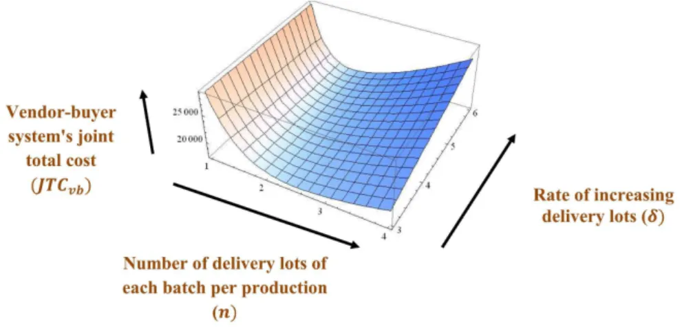
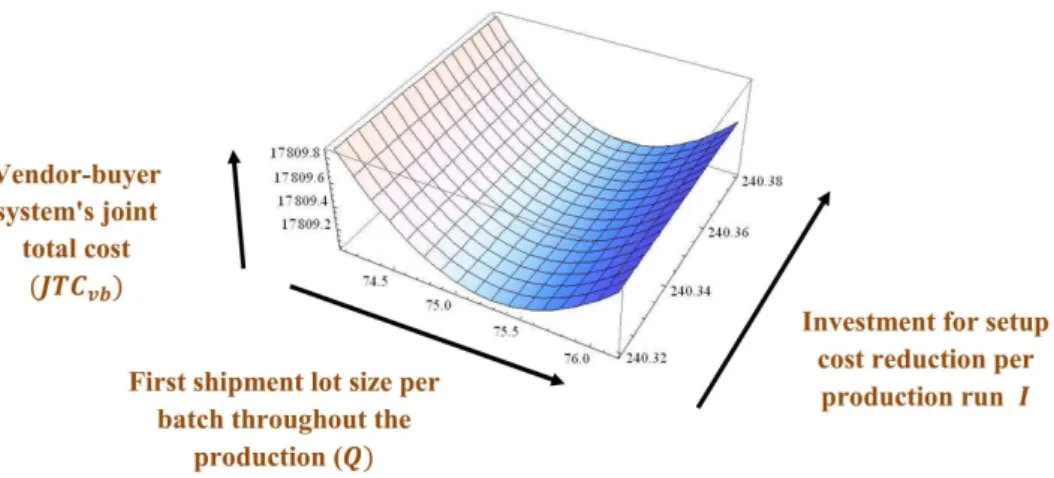
throughout the production Q∗ = 75 units, rate of increasing delivery lots δ∗ = 4 unit/year, and number of delivery lots of each batch per productionn∗=2, and investment for setup cost reduction per production runI∗=$240.34/production run, see Figures2–7for graphical representations of the total cost with optimum values.
Figure 2. Graphical representation of vendor-buyer system’s joint total cost(JTCvb)versus rate of
increasing delivery lots (δ) and investment for setup cost reduction per production runI, whennand Qare fixed,δandIare variable.
Figure 3. Graphical representation of vendor-buyer system’s joint total cost(JTCvb)versus rate of
Figure 4.Graphical representation of vendor-buyer system’s joint total cost(JTCvb)versus number of
delivery lots of each batch per production (n) and investment for setup cost reduction per production run (I), whenQandδare fixed,nandIare variable.
Figure 5.Graphical representation of vendor-buyer system’s joint total cost(JTCvb)versus number of
delivery lots of each batch per production (n) and rate of increasing delivery lots (δ), whenQandIare fixed,nandδare variable.
Figure 6.Graphical representation of vendor-buyer system’s joint total cost(JTCvb)versus number
Figure 7. Graphical representation of vendor-buyer system’s joint total cost(JTCvb)versus first
shipment lot size per batch throughout the production (Q) investment for setup cost reduction per production run (I), whennandδare fixed,QandIare variable.
5.1. Sensitivity Analysis
The sensitivity analysis conducted for the key parameters.
This section illustrates sensitivity analysis, which shows (Table3) the impact of each parameters which areVi,Ui,F,Vt,ρ,hv,Cv,hb1,hb2, andAb, respectively on vendor-buyer system’s joint total
costJTCvb.
Table 3.Sensitivity analysis of key parameters of the model with equal power.
Parameters Changes (in%) JTCvb Parameters Changes (in%) JTCvb
−50% −0.09 −50% −0.07 −25% −0.04 −25% −0.04
Vi +25% 0.04 Cv +25% 0.04
+50% 0.09 +50% 0.07
−50% −0.06 −50% −2.31 −25% −0.03 −25% −1.14
Ui +25% 0.03 Ab +25% 1.10
+50% 0.06 +50% 2.17
−50% −0.003 −50% −3.70
−25% −0.001 −25% −1.80
F +25% 0.001 Vt +25% 1.72
+50% 0.003 +50% 3.37
−50% −2.64 −50% −29.83
−25% −1.30 −25% −14.98
hb1 +25% 1.25 ρ +25% 15.13
+50% 2.46 +50% 30.41
−50% −3.55 −50% −3.70 −25% −1.73 −25% −1.80
hb2 +25% 1.66 hv +25% 1.72
+50% 3.25 +50% 3.37
• The vendor-buyer system’s joint total costJTCvbincreases while unit and variable inspection costs
i.e.,UiandViincrease. On the other hand, if unit transportation costFand variable transportation
costVtare increased, then vendor-buyer system’s joint total costJTCvbis also increased.
• If defective rateρ, vendor’s holding costhv, and vendor’s fixed carbon-emission costCvincrease,
• Increasing values in buyer’s holding cost for perfect itemshb1, holding cost for imperfect itemshb2,
and buyer’s ordering costAbimply that vendor-buyer system’s joint total costJTCvbis increased.
It is found that the negative percentage changes for these three parametershb1,hb2,Abare much
more sensitive than the positive percentage changes.
5.2. Numerical Example by Using Stackelberg Approach Case 1. Buyer as leader and vendor as follower
Example 2. D = 1000 units/year, P = 4000 units/year, Ab = $300/order, A3 = $100/shipment, Cv = $5/delivery, F = $0.2/shipment, Vt = $0.1/unit, Vi = $1/delivery, Ui = $0.2/unit item inspected, Rv = $15/unit,ρ = 0.55, Vv = $5/unit, hb1 = $35/unit/year, hb2 = $30/unit/year, hv = $20/unit/year, α=3500units/year,κ=0.0014, and V0=$1000/setup.
Hence, vendor-buyer system’s joint total costJTCvb=$17, 131.36, first shipment lot size per batch
throughout the production Q∗ = 58 units, rate of increasing delivery lots δ∗ = 3 unit/year, and number of delivery lots of each batch per productionn∗=3, and investment for setup cost reduction per production runI∗=$240.34/production run.
The results, which are obtained in our paper, are compared with the paper of Sarkar et al. [44]. In Sarkar et al. [44], vendor-buyer system’s joint total cost isJTCvb =$24, 045.8 which is larger in
compared to this model. Therefore, this proposed model formulates more appropriate results than Sarkar et al. [44] by incorporating the Stackelberg approach.
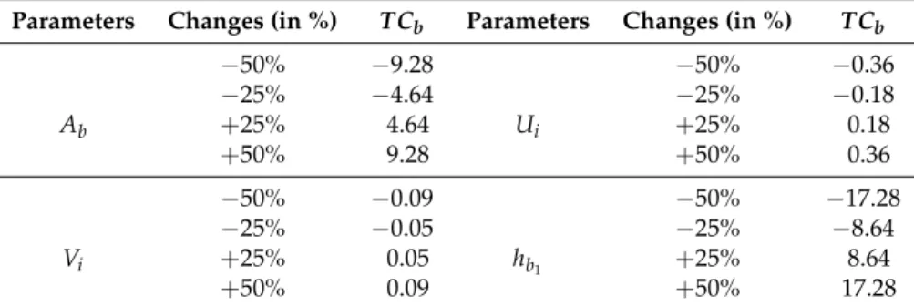
This section discusses the effect on the total cost for buyerTCbby changing several parameters
such asAb,Vi,Ui, andhb1, respectively (see Table4).
• For the parameterAb, which is buyer’s ordering cost, negative and positive percentage changes
are similar. If the value of the parameter Ab increases that indicates buyer’s total cost TCb
also increases.
• It is observed if unit inspection costUiand variable inspection costViare increased, then buyer’s
total costTCbalso increases.
• When buyer’s holding cost for perfect items, i.e.,hb1 increases, then buyer’s total cost TCb is
increased. Both negative percentage change and positive percentage changes are similar for this parameter.
Table 4.Sensitivity analysis for buyer’s cost.
Parameters Changes (in %) TCb Parameters Changes (in %) TCb
−50% −9.28 −50% −0.36 −25% −4.64 −25% −0.18
Ab +25% 4.64 Ui +25% 0.18
+50% 9.28 +50% 0.36
−50% −0.09 −50% −17.28
−25% −0.05 −25% −8.64
Vi +25% 0.05 hb1 +25% 8.64
+50% 0.09 +50% 17.28
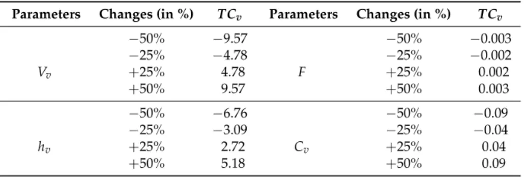
This section allows sensitivity analysis for evaluating the effect of several parameters such asVv, hv,F, andCv, respectively on vendor’s total costTCv(see Table5).
• If the vendor’s variable carbon-emission costVvincreases, then the vendor’s total costTCvalso
increases. In this case, both negative percentage change and positive percentage changes are equal.
• When vendor’s holding costhvincreases, then the vendor’s total costTCvincreases. The negative
• As vendor’s fixed transportation cost F increases, then the vendor’s total costTCvalso increases.
Both the positive and negative percentage changes are same.
• An increasing value in the vendor’s fixed carbon-emission cost per deliveryCvincreases, the total
cost for vendorTCvincreases. For this parameter, the positive percentage change is smaller than
the negative percentage change.
Table 5.Sensitivity analysis for vendor’s cost.
Parameters Changes (in %) TCv Parameters Changes (in %) TCv
−50% −9.57 −50% −0.003
−25% −4.78 −25% −0.002
Vv +25% 4.78 F +25% 0.002
+50% 9.57 +50% 0.003
−50% −6.76 −50% −0.09 −25% −3.09 −25% −0.04
hv +25% 2.72 Cv +25% 0.04
+50% 5.18 +50% 0.09
Case 2. Vendor as leader and buyer as follower.
Example 3. All parameters for this model are as follows:
D = 1000 units/year, P = 4000 units/year, Ab = $300/order, A3 = $100/shipment, Cv = $5/delivery, F = $0.2/shipment, Vt = $0.1/unit, Vi = $1/delivery,Ui = $0.2/unit item
inspected, Rv = $15/unit, ρ = 0.55, Vv = $5/unit, hb1 = $35/unit/year, hb2 = $30/unit/year,
hv=$20/unit/year,α=3500 units/year,κ =0.0014, andV0=$1000/setup.
Hence, the vendor-buyer system’s joint total cost is JTCvb = $17456.1, first shipment lot size
per batch throughout the production isQ∗=28 units, rate of increasing delivery lots isδ∗= 3 unit/year, and number of delivery lots of each batch per production isn∗ =3, and investment for setup cost reduction per production run isI∗=$240.34/production run.
This section analyzes the effect on the buyer’s total costTCbby changing key parameters such as Vi,Ui,hb1, andhb2 (see Table6).
• It is found while unit inspection costUiand variable inspection costViare increased, it implies
the buyer’s total costTCbis also increased.
• The increasing values in buyer’s holding cost for perfect itemshb1 and buyer’s holding cost for
imperfect itemshb2 indicates the increasing value of the buyer’s total costTCb. For this parameter,
the negative percentage change is greater than the positive percentage change.
Table 6.Sensitivity analysis for buyer’s cost.
Parameters Changes (in %) TCb Parameters Changes (in %) TCb
−50% −0.24 −50% −11.27
−25% −0.12 −25% −5.46
Vi +25% 0.12 hb1 +25% 5.18
+50% 0.24 +50% 10.11
−50% −0.46 −50% −15.32
−25% −0.23 −25% −7.34
Ui +25% 0.23 hb2 +25% 6.83
+50% 0.46 +50% 13.25
• If the vendor’s fixed and variable carbon-emission costs i.e.,CvandVvincrease, then the vendor’s
total costTCvalso increases. It is observed that the negative percentage change as well as the
positive percentage changes are similar.
• For the increasing value in vendor’s rework costRvand vendor’s holding costhvindicate vendor’s
total costTCvincreases. LikeCvandVv, both negative percentage change and positive percentage
change are equal forRvandhv.
Table 7.Sensitivity analysis for vendor’s cost.
Parameters Changes (in %) TCv Parameters Changes (in %) TCv
−50% −0.17 −50% −2.61 −25% −0.09 −25% −1.31
Cv +25% 0.09 hv +25% 1.31
+50% 0.17 +50% 2.61
−50% −8.99 −50% −26.98
−25% −4.50 −25% −13.49
Vv +25% 4.50 Rv +25% 13.49
+50% 8.99 +50% 26.98
By analyzing the above comparison Tables8and9, it can be observed that the model with Stackelberg approach gives the lowest vendor-buyer system’s joint total costJTCvbwhen compared
with the model without Stackelberg approach.
Table 8.Model without Stackelberg approach.
Joint total cost $17,809
Table 9.Model with Stackelberg approach.
Description Buyer Cost Vendor Cost Joint Total Cost
Buyer as leader and vendor
as follower $2761.06 $14,370.3 $17,131.36 Vendor as leader and buyer
as follower $2165.7 $15,290.4 $17,456.1
6. Conclusions
Author Contributions:Biswajit Sarkar developed the concept of this model. Sharmila Saren and Mitali Sarkar wrote the whole paper and solved the solution technique of this research. Yong Won Seo contributed several valuable suggestions for this research topic.
Conflicts of Interest:The authors declare no conflict of interest.
Appendix A
R1 = (P−D) 2P −
(1−ρ)2
2 −
ρD
α
R2 = 2Dαρhb2+ (1−ρ)
2h
b1
R3 = Cv+F+Vi R4 = Dρ(Vv+Vt+Rv) Appendix B
The second order partial derivatives of vendor-buyer system’s joint total costJTCvbat the optimal
valuesI∗,Q∗,δ∗, andn∗are given by
∂2JTCvb(n∗,Q∗,δ∗,I∗)
∂I∗2 =
2DV0κ2 2Q+δQn(n−1)e
−κI>0.
∂2JTCvb(n∗,Q∗,δ∗,I∗)
∂Q∗2 =
4DQn(n−1)
(2+δn(n−1))2(V0e
−κI+nR
3+I+Ab)
∂2JTC
vb(n∗,Q∗,δ∗,I∗)
∂δ∗2 =
n(n−1)Q
(2+δn(n−1))
h
R2(2n−1)
3 −
2δ(2n3−3n2+n) 3(2+δn(n−1))
+ 2(n2−n) (2+δn(n−1))2
1+δ2n(n−1)(2n−1) 6
+ 4Dn(n−1)(V0e−
κI+nR
3+I+Ab) (2Q+δn(n−1)Q)2
i
∂2JTC
vb(n∗,Q∗,δ∗,I∗)
∂n∗2 =
4DδQ
(2+δn(n−1))2((R3(1−2n) +V0e
−κI+nR
3+I+Ab)δQ(2n−1)2)
+ hvR1δQ+
R2 (2+δn(n−1))
h
−2δ
1+δ2(2n3−3n2+n) 6
+Q(2n
− 1)−(6n
2−6n+1)δ(2n−1)
6 +
δ(2n−1)
(2+δn(n−1))2
(2n−1)
− Qδ
2(6n2
−6n+1)
6
i
∂2JTCvb(n∗,Q∗,δ∗,I∗)
∂I∗∂Q∗ =
∂2JTCvb(n∗,Q∗,δ∗,I∗)
∂Q∗∂I∗ =−
4D
2Q+δQn(n−1)](1−V0κe
−κI)
∂2JTCvb(n∗,Q∗,δ∗,I∗)
∂I∗∂δ∗ =
∂2JTCvb(n∗,Q∗,δ∗,I∗)
∂δ∗∂I∗ =−
2DQn(n−1)
(2Q+δn(n−1)Q)2(1−V0κe
−κI)
∂2JTCvb(n∗,Q∗,δ∗,I∗)
∂I∗∂n∗ =
∂2JTCvb(n∗,Q∗,δ∗,I∗)
∂n∗∂I∗ =−
2DδQ(2n−1)
(2Q+δQn(n−1))2(1−V0κe
∂2JTCvb(n∗,Q∗,δ∗,I∗)
∂Q∗∂n∗ =
∂2JTCvb(n∗,Q∗,δ∗,I∗) ∂n∗∂Q∗ = hvR1δ(1−2n)
2 −Y
h (2n−1)δ
(2+δn(n−1))2
1+δ2(2n3−3n2+n) 6
+ δ2(6n2−6n+1) 6(2+δn(n−1))
i
− 2D
Q2(2+δn(n−1))
(V
0e−κI+nR3+I+Ab) (2+δn(n−1))
− R3
∂2JTCvb(n∗,Q∗,δ∗,I∗)
∂Q∗∂δ∗ =
∂2JTCvb(n∗,Q∗,δ∗,I∗) ∂δ∗∂Q∗
= hvR1(2n−1)
2 −
2Dn(n−1)
Q2(2+δn(n−1))2(V0e−
κI+nR
3+I+Ab)
− R2n(n−1)
(2+δn(n−1))2
δ2(2n3−3n2+n)
6 +1
+2δ(2n3−3n2+n)R2 6(2+δn(n−1))
∂2JTCvb(n∗,Q∗,δ∗,I∗)
∂n∗∂δ∗ =
∂2JTCvb(n∗,Q∗,δ∗,I∗) ∂δ∗∂n∗
= (V0e−κI+nR3+I+Ab)
2DQ(2n−1)
(2Q+δQn(n−1))2
1+ 2δ(n2−n) (2+δ(n2−n))
+ hvR1(2n−1)Q
2 +R2
hδQ(6n2−6n+1)
3(2+δn(n−1)) −
Q(2n−1)
(2+δn(n−1))2
1
+ δ2(2n3−3n2+n) 6
1−2+2n(nδn(n−1) −1)
− δ
2nQ(n−1) (2+δn(n−1))2
(2n−1)2
3
+ (6n2−6n+1) 6
i
References
1. Chang, H.C.; Ho, C.H.; Ouyang, L.Y.; Su, C.H. The optimal pricing and ordering policy for an integrated inventory model when trade-credit linked to order quantity.Appl. Math. Model.2009,33, 2978–2991. 2. Yang, M.F. Supply chain integrated-inventory model with present value and dependent crashing cost is
polynomial.Math. Comput. Model.2010,51, 802–809.
3. Hoque, M.A. A vendor-buyer integrated-production-inventory model with normal distribution of lead time. Int. J. Prod. Econ.2013,144, 409–417.
4. Jha, J.K.; Shanker, K. An integrated-inventory problem with transportation in a divergent supply chain under service-level constraint.J. Manuf. Syst.2014,33, 462–475.
5. Sarkar, B.; Gupta, H.; Chaudhuri, K.S.; Goyal, S.K. An integrated-inventory model with variable lead time, defective units and delay-in-payments.Appl. Math. Comput.2014,237, 650–658.
6. Ouyang, L.Y.; Ho, C.H.; Su, C.H.; Yang, C.T. An integrated inventory model with capacity constraint and ordersize dependent trade-credit.Comput. Ind. Eng.2015,84, 133–143.
7. Sarkar, B.; Mondal, B.; Sarkar, S. Quality improvement and backorder price discount under controllable lead time in an inventory model.J. Manuf. Syst.2015,35, 26–36.
8. Sarkar, B. Supply chain coordination with variable backorder, inspections and discount policy for fixed lifetime products.Math. Probl. Eng.2016,2016, 6318737.
9. Ahmad, W.; Sofiana, A.; Kurdhi, N.; Laksono, P.W. An integrated inventory model for supplier-manufacturer-retailer system with imperfect quality and inspection errors. Int. J. Logist. Syst. Manag. 2016, doi:10.1504/IJLSM.2016.076893.
11. Liou, Y.C.; Schaible, S.; Yao, J.C. Supply chain inventory management via a stackelberg equilibrium.J. Ind. Manag. Optim.2006,2, 81–94.
12. Yu, Y.; Huang, G.Q.; Liang, L. Stackelberg game-theoretic model for optimizing advertising, pricing and inventory policies in vendor managed inventory (VMI) production supply chains.J. Comput. Ind. Eng.2009, 57, 368–382.
13. Yu, Y.; Chu, F.; Chen, H. A Stackelberg game and its improvement in a VMI system with a manufacturing vendor.Eur. J. Oper. Res.2009,192, 929–948.
14. Zhou, Y.W.; Zhou, D. Determination of the optimal trade credit policy: A supplier-stackelberg model.J. Oper. Res. Soc.2013,64, 1030–1048.
15. Wang, Y.; Sun, X.; Meng, F. On the conditional and partial trade-credit policy with capital constraints: A stackelberg model.Appl. Math. Model.2016,40, 1–18.
16. Taleizadeh, A.A.; Noori-daryan, M.; Govindan, K. Pricing and ordering decisions of two competing supply chains with different composite policies: A Stackelberg game-theoretic approach.Int. J. Prod. Econ.2016, doi:10.1080/00207543.20.
17. Wang, D.; Du, G.; Jiaob, R.J.; Wu, R.; Yu, J.; Yang, D. A Stackelberg game theoretic model for optimizing product family architecting with supply chain consideration.Int. J. Prod. Econ.2016,172, 1–18.
18. Denizel, M.; Erengü´cc, S.; Benson, H.P. Dynamic lot-size with setup cost reduction.Eur. J. Oper. Res.1997, 100, 537–549.
19. Diaby, M. Integrated batch size and setup reduction decisions in multi product, dynamic manufacturing environments.Int. J. Prod. Econ.2000,67, 219–233.
20. Nyea, T.J.; Jewkes, E.M.; Dilsc, D.M. Theory and Methodology Optimal investment in setup reduction in manufacturing systems with WIP inventories.Eur. J. Oper. Res.2001,135, 128–141.
21. Freimer, M.; Thomas, D.; Tyworth, J. The value of setup cost reduction and process improvement for the economic production quantity model with defects.Eur. J. Oper. Res.2006,173, 241–251.
22. Huang, C.K.; Cheng, T.L.; Kao, T.C.; Goyal, S.K. An integrated inventory model involving manufacturing setup cost reduction in compound Poisson process.Int. J. Prod. Econ.2011,49, 1219–1228.
23. Annadurai, K.; Uthayakumar, R. Controlling setup cost in (Q,r,L) inventory model with defective items. Appl. Math. Model.2010,34, 1418–1427.
24. Sarkar, B.; Majumder, A. Integrated vendor-buyer supply chain model with vendor’s setup cost reduction. Appl. Math. Comput.2013,224, 362–371.
25. Sarkar, B.; Moon, I. Improved quality, setup cost reduction, and variable backorder costs in an imperfect production process.Int. J. Prod. Econ.2014,155, 204–213.
26. Sarkar, B.; Chaudhuri, K.S.; Moon, I. Manufacturing setup cost reduction and quality improvement for the distribution free continuous-review inventory model with a service level constraint.J. Manuf. Syst.2015,34, 74–82.
27. Allahverdi, A. The third comprehensive survey on scheduling problems with setup times/costs. Eur. J. Oper. Res.2015,246, 345–378.
28. Priyan, S.; Uthayakumar, R. Setup cost reduction EMQ inventory system with probabilistic defective and rework in multiple shipments management.Int. J. Syst. Assur. Eng. Manag.2016, doi:10.1007/s13198-016-0418-2. 29. Sarkar, B.; Majumder, A.; Sarkar, M.; Dey, B.K.; Roy, G. Two-echelon supply chain model with manufacturing
quality improvement and setup cost.J. Ind. Manag. Opt.2016, doi:10.3934/jimo.2016063.
30. Sarkar, B.; Sett, B.K.; Roy, G.; Goswami, A. Flexible setup cost and deterioration of products in a supply chain model.Int. J. Appl. Comput. Math.2016,2, 25–40.
31. Mason, S.J.; Ribera, P.M.; Farris, J.A.; Kirk, R.G. Integrating the warehousing and transportation functions of the supply chain.Trans. Res. Part E2003,39, 141–159.
32. Hill, J.; Galbreth, M. A heuristic for single-warehouse multi retailer supply chains with all-unit transportation cost discounts.Eur. J. Oper. Res.2008,187, 473–482.
33. Kang, J.H.; Kim, Y.D. Coordination of inventory and transportation managements in a two-level supply chain.Int. J. Prod. Econ.2010,123, 137–145.
34. Chan, T.S.; Zhang, T. The impact of collaborative transportation management on supply chain performance: A simulation approach felix.Expert Syst. Appl.2011,38, 2319–2329.
![Figure 1. Inventory positions of buyer. Adapted from Sarkar et al. [ 44 ].](https://thumb-ap.123doks.com/thumbv2/123deta/6882353.248234/10.892.235.663.152.452/figure-inventory-positions-buyer-adapted-sarkar-et-al.webp)