[DOI: 10.2197/ipsjjip.25.486]
Regular Paper
Particle-based Shallow Water Simulation with Splashes
and Breaking Waves
M
akoto
F
ujisawa
1,a)T
akuya
N
akada
1M
asahiko
M
ikawa
1,b)Received: September 6, 2016, Accepted: March 3, 2017
Abstract: We propose a fast method of simulating large-scale liquid phenomena by coupling 2D and 3D smoothed particle hydrodynamics (SPH). Our method combines 2D SPH-based shallow water simulation with 3D SPH simula-tion to effectively treat complex behaviors, such as splashes and breaking waves. To achieve realistic animasimula-tion, we generate 3D particles from 2D particles by categorizing these particles according to motion and position. One-way interactions between both types of particles are described by the conservation of momentum. We demonstrate the effectiveness of our approach in various graphical scenes.
Keywords: large-scale fluid simulation, shallow water, SPH
1.
Introduction
Fluid simulation is widely used to create computer graphics animation of complex natural phenomena. However, it is diffi -cult to compute the details of large phenomena, such as floods and ocean waves, in real-time because of the high computational cost, while interactive applications, such as games, require both high levels of detail and very fast computing. One approach to this type of application is to use a two-dimensional height field, in which three-dimensional fluid behaviors are approximated as surface wave motion. The wave motion is calculated as a two-dimensional flow on a surface, which dramatically reduces the computational cost. However, this method cannot represent some motions characteristic of waves, such as splashes and breaking waves, because it can only treat vertical movement.
In this paper, we propose a new method that realizes fast fluid simulation with finer details by combining two-dimensional shallow-water simulation with particles and three-dimensional smoothed particle hydrodynamics (SPH). A height field repre-sented by the particles is updated according to the shallow wa-ter equation (SWE) and three-dimensional particles are generated by analyzing wave movement. Both particles can be naturally combined because the full Lagrangian representation is available. Also, we propose to use a screen-space rendering technique to represent a water surface by using additional particles for render-ing in cases where the particle-based shallow-water simulation would cause holes due to an insufficient number of particles.
2.
Related Work
For large-scale water simulation, various methods have been proposed. Using a two-dimensional height field instead of a full three-dimensional fluid solver is the most popular solution for
1 University of Tsukuba, Tsukuba, Ibaraki 305–8550, Japan a) fujis@slis.tsukuba.ac.jp
b) mikawa@slis.tsukuba.ac.jp
interactive applications. Several papers propose using the fast Fourier transform (FFT) to construct a height field and create fluid animations in large-scale scenes with a high level of de-tail [18], [25], [26]. Kass and Miller [12] introduced a wave equa-tion that can determine water surface movement using a height-field representation. This approach is not based on physics, but it can very effectively simulate large-scale water scenes, such as ocean waves. Later researchers extended this technique to fluid splashing [22], bubbles and droplets [19], waves over ter-rain [8], [17], and hydraulic erosion [28].
large-method based on SPH shallow-water simulation [23], which we extend to three-dimensional effects by using SPH particles. Both the water surface and three-dimensional effects are represented as particles, so that we can easily combine the simulation, and the method has the advantage of being a particle-based method. Also, we propose a method to calculate interactions on the ba-sis of momentum conservation from three-dimensional to two-dimensional particles.
There are many works that consider the full three-dimensional simulation of liquid by using a grid [3] or particles [11]. SPH [6], which is one popular particle-based simulation method, has been widely used for computer graphics [11], [20] because of its sim-plicity and the ease of extending the simulation space. SPH uses an explicit calculation of pressure according to a state equation, which allows very fast computation but causes incompressibil-ity problems. To solve this problem, various algorithms, such as WCSPH [1], PCISPH [24], IISPH [10], PBF [16], and DFSPH [2] have been developed. We use PBF (Position-Based Fluid) to sim-ulate the behavior of three-dimensional particles because of its handling of incompressibility and its low computational cost rel-ative to other volume-conserving methods.
3.
Method
We use SWE with particles [23] to simulate the water wave. This two-dimensional simulation cannot generate any three-dimensional effects, such as breaking waves or splashing. To make such kinds of effects, we introduce particles that move freely in three-dimensional space and then use SPH to calculate the behavior of these particles. The particles are generated via analysis of the movement of SWE particles and deleted when they enter into the water’s surface. Finally, both types of particles are rendered by a screen-space rendering technique. In the follow-ing sections, we call the particles used in SWE simulation the 2D particles, and those used in three-dimensional PBF are called 3D particles.
3.1 Particle-based Shallow Water Simulation
In general shallow-water simulation, the simulation space is partitioned by a two-dimensional grid, and each grid cell has a height, a vertical velocity, and horizontal velocity, and these vari-ables are updated by using the SWE [13]. SWE, used for repre-senting the motion of the water surface, is based on the Navier– Stokes equations, meaning that the system represents mass and momentum conservation. The velocity field is updated by solv-ing the SWE (2) and then changsolv-ing the height field on the basis of the velocity Eq. (1).
∂h
∂t =−∇ ·(hu) (1)
Du
Dt =−g∇(h+H(x))+aext (2)
wherehis the height of the water surface,uis the velocity of the
mine the height of the particles.
hi=
ρ2D i
ρ0
(3)
wherehiandρ2iDare the height from the bottom and the density of particlei, respectively. In this,ρ0is the rest density of water. We assume that gravity acts along theyaxis. In this case, 2D par-ticles are placed on thexzplane and the densityρ2D
i is calculated as in 2D SPH.
ρ2D
i =
j∈N
m2D
j Wpoly6(xj−xi,l2D) (4)
whereNis the set of 2D particles within the effective radiusl2D,
m2D
j is the mass of 2D particlej, andW(xj−xi,l2D) is the kernel function. By substituting Eq. (3) into Eq. (2), we can obtain the SWE for the particle method:
∂u2D x z
∂t =−
g ρ0
∇ρ2iD−g∇H(x)+ν∇2u2D
x z +aext (5)
whereu2D
xz is the velocity of a 2D particle on the xzplane and
ν(=µ/ρ0) is the kinematic viscosity coefficient. The termν∇2u2x zD
is a viscosity term used to stabilize the surface motion [14]. Equa-tion (5) updates the velocityu2D
xz of 2D particles with timestep length ∆t, and position x2xzD is also updated from the veloc-ity. Finally, they element of the position is calculated from x2D
y = hi+H(x2xzD) and Eq. (3). The SPH shallow-water simu-lation transforms the change in density to the change in height. We also restrict the velocity by setting a maximum propagation speed of water ghito that given from a wave equation, which creates a more stable simulation.
Boundary handling is a challenging problem of particle-based methods. In our method, we use boundary particles to prevent particle stacking near the boundary, which can be caused by un-derestimation of the density. Boundary particles are placed into solid boundaries. As an added step, we set the velocityu2D
xz to 0 for particles that contact the boundary, which represents a one-way interaction from solid to liquid.
3.2 3D Particle Generation
As mentioned, SWE simulation alone cannot simulate 3D ef-fects, such as breaking waves or splashing. In order to consider these kinds of phenomena, we generate 3D particles from 2D par-ticles. In SWE simulation, the motion of water surface would be restricted to vertical movement and it only generates waves. We assume that there are only two types of 3D effect arising from the wave as shown inFig. 1: a splash shot to the upper direction from crest of wave and a plunging breaker (breaking wave) moved to the horizontal direction from side of wave.
Fig. 1 3D effects caused by a wave.
Fig. 2 Classification of newly generated 3D particles and their initial veloc-ities. A blue circle represents a 2D particle and a light blue is a 3D particle.
hi−hiprev
∆t > γ3D. (6)
Here,hiprevis the height of the 2D particleiat the previous step, andγ3Dis the user-specified threshold for 3D particle generation. Each particle satisfying Eq. (6) is classified into one of three types according to the maximum difference in height with neighboring particlesj. This is characterized by
hdi f f =max(hj)−min(hj) (7)
where max(hj) and min(hj) are the maximum and minimum height among neighboring 2D particles. We classify the 2D par-ticle into the three types, “top”, “slope” and “steep” parpar-ticles, by hdi f f as shown inFig. 2. The “top” particle represents a splash generated from the top of the wave, while the “steep” particle represents a plunging breaker generated from the steep region of the wave. We also define the “slope” particle in order to smoothly interpolate the motion of the above two particles. These have the following thresholds: top particles are generated when hdi f f ≤ γtop; steep particles are generated whenγsteep ≤ hdi f f; and splash particles are generated in other cases (i.e., when
γtop<hdi f f < γsteep), where we assume that 0≤γtop≤γsteep. The initial position of a new 3D particle is determined as fol-lows.
x3xzD = x2xzD (8)
x3yD = (1−αheight)h2iD+αheightmax(hj)+H(x2D) (9)
whereαheightis a parameter used to adjust the height of 3D parti-cle. In this paper, we use 0–0.3 forαheight. The initial position is independent of the type of particle. In contrast, the initial velocity of each 3D particle depends on its type.
• “top” particles
The particle is placed near the wave crest when the change of height from the previous timestep is large but the difference between near particleshdi f f is small. In this case, splashes are generated, and we set the vertical vector with the veloc-ity:
Fig. 3 3D particles deletion.
utopxz =0, utopy =ktop
hi−hiprev
∆t
wherektopis the coefficient for “top” particles.
• “steep” particles
The particle is placed on the side of the wave when the dif-ference from nearby particles is large. In this case, we set an oblique velocity to represent a breaking wave.:
usteepxz = a 2D xz
|a2D xz|
ghi, usteepy =ksteep
hi−hiprev
∆t
whereksteepis the coefficient for “steep” particles,a2xzDis the vector of acceleration of the 2D particle in thexzplane, and
ghiis the maximum propagation speed of water as given by a wave equation. We just usea2D
xz to determine the direc-tion of the steep particle movement, because the horizontal velocity of the 2D particle does not correspond to the wave speed.
• “slope” particles
“slope” particles are placed between “top” and “steep,” and the initial velocity is calculated by linear interpolation of the corresponding “top” and “steep” particle velocities:
uslopexyz =αslopeusteepxyz +(1−αslope)utopxyz
whereαslope=(hdi f f−γtop)/(γsteep−γtop) is the interpolation coefficient for “steep” particles,
After 3D particles have been generated from the 2D particles, the positions of the 3D particles are updated by PBF [16]. PBF can enforce the incompressibility of the fluid by imposing a den-sity constraint, such asci(x31D, . . . ,x
3D
N ) = ρ
3D
i /ρ0−1 = 0, on all 3D particles. PBF uses a constraint-based method to obtain a uniform distribution of the particles, rather than the Poisson dis-tribution of pressure that is derived from the Navier–Stokes equa-tions. This might produce unreasonable results, because SWE is based on the Navier–Stokes equations. We think the equation for mass conservation (Eq. (1) for SWE) is unlikely to be a problem because both 2D and 3D simulations use the particles for approx-imation. Also, the pressurepis approximated from the change of heighthasp=gρhin the SWE [13]. This is similar to a position-based method. In our experiments, we did not observe any visual artifacts related to this problem.
3.3 3D Particle Deletion
mi
whereNneighis the number of neighboring 2D particles,rxzis the position of 2D particle relative to the 3D particle on thexzplane. In Eq. (10), the termm2D
i u2xzDrepresents the momentum of a 2D particle before the velocity update; we add the momentum of the relevant 3D particle to it. For this, we assume that the momen-tum of a 3D particlem3D
i u
3D uniformly affects all neighboring
2D particles. Thexzcomponent of the momentum of the 3D par-ticle (m3iDu3xzD/Nneigh) is directly added to the momentum of the 2D particles. Theycomponent of the momentum of 3D particle, in contrast, works as a repulsive force on the 2D particles in the directionrxz/|rxz|.
3.4 Rendering
General height-field approaches use a flat mesh and move the vertices according to the height field. We cannot apply this method to our simulation results because we incorporate 3D par-ticles. Full 3D particle-based methods, in contrast, commonly use the Marching Cubes algorithm [15] to make the surface mesh from a potential field defined by the particles and the kernel func-tion. This technique is valid for 3D particles only, but we also have 2D particles that are characterized by just upper surface in-formation (i.e., a height). To handle this, we create a surface mesh from both 2D and 3D particles by using the Screen Space Meshes (SSM) algorithm [21] for rendering. SSM uses only those particles visible from a specified viewpoint. Therefore, it is not necessary to calculate information about the particles under the surface wave if the viewpoint is above the 2D particles.
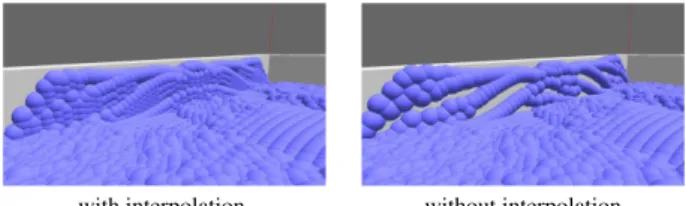
SSM directly projected the particles into screen space and gen-erates a mesh in the 2D space. If the particle distribution is sparse, SSM will generate a mesh with many holes. The particle-based SWE calculates the particle distribution in two dimensional space and then it projects the particles into three dimensional space by computing the height from the density of the particles. Even if there is no hole in two dimensional space, when projecting to three dimensional space with the height, some holes are gener-ated at a region where the density rapidly changes as shown in
Fig. 4. We solve this problem by using a particle interpolation. The holes appear in the side of the wave where the particles are rapidly moving in a vertical direction. In the side of the wave, the particles also move toward to the center of the wave as indi-cated by the red arrow in Fig. 4, because the wave is created by the movement of the particles gathering. As a result, the particles placed on the wave side move along to the wave surface. We make use of this feature to fill the holes.Figure 5shows the particle in-terpolation using the particle movement along the wave surface. We simply use a linear interpolation to deside the position of in-terpolated particles and particle interpolation is performed when the following condition is satisfied.
γinter p<|x2xyDz−x
2Dprev
xyz | (11)
Fig. 4 Holes on surface generated by the vertical movement of the parti-cles. Fully three dimensional simulation generates uniform particle distribution (left), while particle-baesd SWE causes non-uniform dis-tribution in three dimensional space (right).
Fig. 5 Particle interpolation for screen-space mesh creation. A green parti-cle represents an interpolated partiparti-cle.
Fig. 6 Comparison of particle interpolation.
wherex2xDpreyz vis the 3D position of a 2D particle at the previous step, andγinter pis the user-defined threshold for particle interpo-lation. We useγinter p =r2D/2 for all examples wherer2Dis the radius of the 2D particle. If the particle fulfills the condition of Eq. (11), then we place new particles on the straight line connect-ing the previous position to the current position of the 2D parti-cle. In our experiments, the interpolation between the current and previous particles is not enough to cover all holes. So that we extrapolate the particles inside the liquid as shown in Fig. 5 right.
Figure 6shows the result with and without particle interpolation.
4.
Results
This section describes the results of applying the proposed method to several scenes. All results were generated on a com-puter equipped with a 3.7 GHz Intel Core i7 CPU and an NVIDIA GeForce GTX TITAN GPU. The algorithm was predominantly implemented on the GPU by using NVIDIA CUDA. We use the method of Ref. [7] to search for neighboring particles. We set the resolution of the screen to 1280×720 pixels and let∆t=0.005 s in all examples.Table 1lists the parameters used in obtaining the results.
scenar-Fig. 7 Scene1: Dam breaking from the center region. Blue indicates 2D particles and white indicates 3D particles.
Fig. 8 Dam breaking scene with full 3D simulator. Only 3D particles are used to simulate the fluid behavior. Average simulation time per frame is around 1 fps.
Fig. 9 Water drop falling on a water surface.
Table 1 Paramters for all examples.
scene 1 scene 2 scene 3 scene 4
αheight 0.3 0.3 0 0.3
γ3D 3 1.5 3 1
γtop 0.1 0.15 0.07 0.3
γsteep 0.15 0.2 0.15 0.5
ktop 0.3 0.6 0.5 0.35
ksteep 0.2 0.2 0.5 0.05
ios. However, we observe that updating velocity while conserv-ing momentum from 3D to 2D particles makes unnaturally high waves, using simulation with 2D particles only as a baseline.
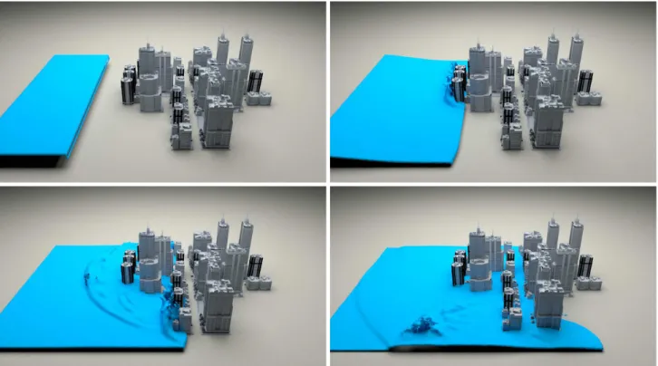
Figure 9shows that this method of velocity update is valid for a scene with falling water drops. In these scenes, conservation of vertical and horizontal momentums works well to generate waves and splashes.Figure 10shows a dam breaking scene with some buildings. Our approach can make plausible animation of large-scale scenes at an interactive rate.
Table 2summarizes the performance of our method including surface mesh creation. Table 2 also includes the result of full 3D simulation. Similar to the proposed method, we implemented the full 3D simulation on the GPU by using the method of the method of Ref. [7] and we set the 3D particles under the water so that it is the same as Scene 1–4. As shown in Table 2, the proposed method succeeded in drastically reducing the number of the par-ticles. As a result, our method is about 9–23 times faster than the full 3D simulation in average fps and about 5–8.5 times faster in maximum fps.Figure 11shows comparisons of the results of Scene 2–4. Parameters for full 3D simulation, such as an effective radius, a mass of particle, are same as the one used for the results of the proposed method.
in-Fig. 10 Scene 4: Dam breaking with buildings.
Table 2 Perfomance results for all examples.
Scene Proposed method Full 3D simulation
2d partices Max. 3d particles Avg. time (fps) Max. time (fps) 3d particles Avg. time (fps)
Scene 1 13,700 35,837 61.1 43.5 286,300 6.29
Scene 2 10,800 8,000 137.5 50.0 243,531 5.83
Scene 3 10,800 8,000 98.1 43.5 244,558 5.73
Scene 4 158,775 142,864 24.3 14.3 1,008,315 2.64
Fig. 11 Comparisons of the results of the proposed method (top) and full three dimensional simulation (bottom).
compressibility. On the other hand, the calculation speed of the proposed method does not decrease, since the method only con-siders the ocean surface. However, the calculation time of the proposed method depends on the number of generated 3D parti-cles as shown inFig. 13. It would cause a temporary decrease in computational speed during simulation.
All resulting animations are included in our movie file putting on our website:
http://slis.tsukuba.ac.jp/pbcglab/files/jip sphswe.mp4
5.
Limitation
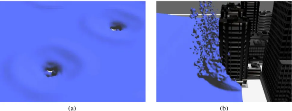
There are some limitations of the proposed method. At first, the interpolation of particles for rendering cannot fulfill all holes.
Fig. 14 Limitations of the proposed method: (a) the particle interpolation cannot prevent the hole made in a concave region, (b) inaccurate wave velocity calculation causes unnatural reflected splashes and breaking waves.
Fig. 12 Comparison of computational time of Scene 1 with full 3D simula-tion.
Fig. 13 Computational time of Scene 1 with the number of 3D particles.
particles move outward around a point. Moreover, the shape of the particles clearly appears when the viewpoint approaches and some flickering artifacts are observed at the inner silhouette of the surface mesh due to the SSM algorithm.
Another limitation is that the velocity direction of the wave calculated in Section 3.2 is not entirely correct. Figure 14 (b) shows a frame from Scene 4 with other parameters:γtop =0.15,
γsteep =0.2,ktop =0.3,ksteep =0.3. The splashes and breaking waves caused from the wave colliding to the building are bounded to the opposite direction of the wave propagation. It is not neces-sarilly the case that the velocity direction of the particles calcu-lated by SWE is equal to the velocity of the wave, because SWE decides a height of wave from the density of the particles.
*1 http://www.mitsuba-renderer.org
6.
Conclusions and Future Work
We have presented a fully Lagrangian simulation method for large-scale phenomena by combining 2D particle-based shallow-water simulation with a 3D SPH fluid simulation method. 3D particles generated by using a classification based on the state of surrounding 2D particles and a system that updates velocity ac-cording to momentum conservation makes it possible to realize various 3D effects, such as breaking waves and splashing.
As future work, we plan to modify the surface mesh creation because the current particle interpolation method is insufficient to fill all holes. We also want to modify flickering artifacts ob-served in the inner silhouette of the surface mesh. It would be caused by the weak silhouette smoothing in SSM [21], while we could not apply a strong smoothing because the shrinking of the inner silhouette caused another artifact. Moreover, the corrected calculation of the wave direction is also a future work.
We currently consider breaking waves and splashing. There are other possible types of 3D effects, such as waterfalls. Moreover, our method cannot treat a scene like pouring water into a glass be-cause we do not consider mass conservation between 2D and 3D particles. Poured water represented by 3D particles will disap-pear under the water surface, without increasing the height of the water. We have to consider another height calculation method to achieve mass conservation because the current height calculation is based on only the density of the 2D particles.
Acknowledgments This work was supported by JSPS KAKENHI Grant Number 25730069 and 16K00148. We also thank to anonymous reviewers for their constructive comments. The images in this paper were rendered using Mitsuba ren-derer*1.
References
[1] Becker, M. and Teschner, M.: Weakly Compressible SPH for Free Sur-face Flows,Proc. 2007 ACM SIGGRAPH/Eurographics Symposium on Computer Animation, pp.209–217 (2007).
[2] Bender, J. and Koschier, D.: Divergence-free Smoothed Particle Hydrodynamics,Proc. 14th ACM SIGGRAPH/Eurographics Sympo-sium on Computer Animation, pp.147–155 (online), DOI: 10.1145/
2786784.2786796 (2015).
[3] Bridson, R.: Fluid Simulation for Computer Graphics, A K Petters (2008).
[4] Chentanez, N. and M¨uller, M.: Real-Time Simulation of Large Bodies of Water with Small Scale Details, Proc. 2010 ACM SIG-GRAPH/Eurographics Symposium on Computer Animation, pp.197– 206 (2010).
[8] Holmberg, N. and W¨unsche, B.C.: Efficient Modeling and Render-ing of Turbulent Water Over Natural Terrain,Proc. 2nd International Conference on Computer Graphics and Interactive Techniques in Aus-tralasia and South East Asia(GRAPHITE ’04), pp.15–22 (online), DOI: 10.1145/988834.988837 (2004).
[9] Ihmsen, M., Akinci, N., Akinci, G. and Teschner, M.: Unified spray, foam and air bubbles for particle-based fluids, The Visual Com-puter, Vol.28, No.6-8, pp.669–677 (online), DOI: 10.1007/ s00371-012-0697-9 (2012).
[10] Ihmsen, M., Cornelis, J., Solenthaler, B., Horvath, C. and Teschner, M.: Implicit Incompressible SPH, IEEE Trans. Visualization and Computer Graphics, Vol.20, No.3, pp.426–435 (online), DOI: 10.1109/TVCG.2013.105 (2014).
[11] Ihmsen, M., Orthmann, J., Solenthaler, B., Kolb, A. and Teschner, M.: SPH Fluids in Computer Graphics,Eurographics 2014 - State of the Art Reports, pp.21–42 (online), DOI: 10.2312/egst.20141034 (2014). [12] Kass, M. and Miller, G.: Rapid, Stable Fluid Dynamics for
Com-puter Graphics,ACM SIGGRAPH Computer Graphics, Vol.24, No.4, pp.49–57 (online), DOI: 10.1145/97880.97884 (1990).
[13] Layton, A.T. and Panne, M.V.D.: A Numerically Efficient and Stable Algorithm for Animating Water Waves,The Visual Computer, Vol.18, No.1, pp.41–53 (2002).
[14] Lee, H. and Han, S.: Solving the Shallow Water Equations Using 2D SPH Particles for Interactive Applications,The Visual Computer, Vol.26, No.6-8, pp.865–872 (2010).
[15] Lorensen, W.E. and Cline, H.E.: Marching Cubes: A High Resolu-tion 3D Surface CconstrucResolu-tion Algorithm, ACM SIGGRAPH Com-puter Graphics, Vol.21, No.4, pp.163–169 (1987).
[16] Macklin, M. and M¨uller, M.: Position Based Fluids, ACM Trans. Graphics, Vol.32, No.4, pp.104:1–104:12 (online), DOI: 10.1145/
2461912.2461984 (2013).
[17] Maes, M.M., Fujimoto, T. and Chiba, N.: Efficient Animation of Wa-ter Flow on Irregular Terrains,Proc. 4th International Conference on Computer Graphics and Interactive Techniques in Australasia and Southeast Asia(GRAPHITE ’06), pp.107–115, ACM (online), DOI: 10.1145/1174429.1174447 (2006).
[18] Mastin, G.A., Watterberg, P.A. and Mareda, J.F.: Fourier Synthe-sis of Ocean Scenes, IEEE Computer Graphics and Applications, Vol.7, No.3, pp.16–23 (online), DOI: doi.ieeecomputersociety.org/
10.1109/MCG.1987.276961 (1987).
[19] Mould, D. and Yang, Y.-H.: Modeling Water for Computer Graph-ics,Computers&Graphics, Vol.21, No.6, pp.801–814 (online), DOI: 10.1016/S0097-8493(97)00059-9 (1997).
[20] M¨uller, M., Charypar, D. and Gross, M.: Particle-Based Fluid Simulation for Interactive Applications, Proc. 2003 ACM SIG-GRAPH/Eurographics Symposium on Computer Animation, pp.154– 159 (2003).
[21] M¨uller, M., Schirm, S. and Duthaler, S.: Screen Space Meshes,Proc. 2007 ACM SIGGRAPH/Eurographics Symposium on Computer Ani-mation, pp.9–15 (2007).
[22] O’Brien, J.F. and Hodgins, J.K.: Dynamic Simulation of Splashing Fluids,Proc. Computer Animation 95, pp.125–132 (1995).
[23] Solenthaler, B., Bucher, P., Chentanez, N., M¨uller, M. and M.Gross: SPH Based Shallow Water Simulation,Proc. Virtual Reality Interac-tions and Physical SimulaInterac-tions(VRIPhys), pp.39–46 (2011). [24] Solenthaler, B. and Pajarola, R.: Predictive-corrective
Incompress-ible SPH,ACM Trans. Graphics, Vol.28, No.3, pp.40:1–40:6 (online), DOI: 10.1145/1531326.1531346 (2009).
[25] Tessendorf, J.: Simulating Ocean Water, SIGGRAPH 1999 course notes(1999).
[26] Thon, S., Dischler, J.-M. and Ghazanfarpour, D.: Ocean Waves Synthesis Using a Spectrum-based Turbulence Function,Proc. Com-puter Graphics International 2000, pp.65–72 (online), DOI: 10.1109/
CGI.2000.852321 (2000).
[27] Th¨urey, N., M¨uller-Fischer, M., Schirm, S. and Gross, M.: Real-time Breaking Waves for Shallow Water Simulations, Proc. 15th Pacific Conference on Computer Graphics and Applications, pp.39–46 (on-line), DOI: 10.1109/PG.2007.54 (2007).
[28] ˇSt’ava, O., Beneˇs, B., Brisbin, M. and Kˇriv´anek, J.: Interactive Terrain Modeling Using Hydraulic Erosion,Proc. 2008 ACM SIG-GRAPH/Eurographics Symposium on Computer Animation, pp.201– 210 (2008).
chanical engineering from Shizuoka Uni-versity in 2003, 2005, and 2008 respec-tively. He worked for Nara Institute of Science and Technology from 2008 to 2010 as an Assistant Pro-fessor. His research interests include computer graphics and physics simulation. He is a member of ACM, IEEE CS, IIEEJ, IPSJ and VRSJ.
Takuya Nakadareceived B.A. degree from University of Tsukuba in 2015. He is currently working in the NHN hangame Corp. since 2015. His research interests include computer graphics and physics simulation.