2015, International Economics (1)
Jun Oshiro
∗object We learn the principle of international economics to do your master thesis. support page
https://sites.google.com/site/junoshiro5urban/home/lectures/gradtrade2015 grade Write an essay on the course.
requirement Mathematics (real analysis and linear algebra) and English (to read articles) to some extent.
References
textbook
(1) P.R. Krugman, M. Obstfeld and M.J. Melitz (2014) “International Economics: Theory
& Policy (10th ed.),” Pearson Education.
Krugman et al. (henceforth, KOM) is a well-known and widely-used book for undergraduate courses all over the world. This is a good book to own. But we will not really use this so that you don’t need to buy this. There is a Japanese-translated edition, however, which contains lots of mistranslations and is based on the out-of-date edition.
supplementary books
(1) Feenstra, R. C. (2004) “Advanced International Trade,” Princeton Univ Press.
(2) Feenstra, R. C. and A. M. Taylor (2011) “International Economics (2nd edition)” Worth.
(3) 阿部顕三・遠藤正寛 (2012) 『国際経済学』有斐閣
(4) 多和田眞 (2012)『コンパクト国際経済学』新世社
∗Department of Law and Economics, Okinawa University. email: [email protected]
microeconomics and mathematics
(1) 尾山大輔・安田洋祐 (2013) 『改訂版 経済学で出る数学: 高校数学からきちんと攻める』
日本評論社
(2) 林貴志 (2013) 『ミクロ経済学 (増補版)』ミネルヴァ書房
(3) D. クレプス (2008) 『MBA のためのミクロ経済学入門』東洋経済新報社
(4) D. クレプス (2009) 『MBA のためのミクロ経済学入門 2』東洋経済新報社
(5) P.クルーグマン, R. ウェルズ (2007) 『クルーグマン ミクロ経済学』 東洋経済新報社
(6) H. R. ヴァリアン (2007) 『入門ミクロ経済学』 勁草書房
(7) G. A. Jehle and P. J. Reny (2011) “Advanced Microeconomic Theory (3rd ed.),” Pearson. (8) J. G. Riley (2012) “Essential Microeconomics,” Cambridge Univ Press.
(9) H. R. Varian (1992) “Microeconomic Analysis (3rd ed.),” W.W. Norton and Co.
international finance and macroeconomics
(1) 小川英治・川崎健太郎 (2007) 『MBA のための国際金融』有斐閣
(2) 齊藤誠・岩本康志・太田聰一・柴田章久 (2010) 『マクロ経済学』 有斐閣
(3) 中田真佐男 (2011) 『基礎から学ぶ動学マクロ経済学に必要な数学』日本評論社
(4) M. Obstfeld and K. Rogoff (1996) “Foundations of International Macroeconomics,” The MIT Press.
econometrics
(1) 浅野皙・中村二朗 (2009) 『計量経済学』有斐閣
(2) J. H. Stock and M. W. Watson (2010) Introduction to Econometrics (3rd ed.), Addison- Wesley.
(3) J. M. Wooldridge (2013) Introductory Econometrics: A Modern Approach (5th ed.), Cengage Learning.
1 The Gravity Model (KOM, ch2)
point Distance has not been dead yet.
1.1 Simple but robust relations
Gravity equations are an empirical model of bilateral transactions. For half of a century, they have been used to estimate econometrically the effect of preferential trade blocs, national border, language, and other measure of trade frictions on trade flows.1
By analogy with the Newtonian gravity model, the observed volume of trade between any two countries can be expressed by
Tij = AY
a i Yjb
Dijc uij, (1)
where Tij is the (nominal) trade flow from country i to country j, Yi is the (nominal) income of country i, Dij is the distance between the two countries, uij is an error term, and A > 0, a, b, c are constant. We estimate the following monotonic transformation
ln Tij = ln A + a ln Yi+ b ln Yj− c ln Dij + ln uij. (2) The softwares like R, STATA, MS Excel, EView, SPSS, or GAUSS give the user OLS estimators of the parameters, ˆa, ˆb, and ˆc. Usually, we will find the signs of ˆa, ˆb, and ˆc are significantly positive. That is, other things being equal, the trade flows between any economies are larger, the larger is either economy; In addition, trade is negatively affected by “spatial frictions.”
Across many studies, the model has notable power to fit the data in the sense that the regression explains a lot of the variation, usually 80–90%, in the trade flows. So the gravity equation has actually established itself as the most successful and celebrated empirical model in international trade. It appears to imply that whenever we think about trade, we should have a model reconciling the empirical relationship represented by Eq. (1) in our mind. Alas, textbook models of traditional trade theory focusing on comparative advantages without trade frictions fails to do so. Ricard and Heckscher-Ohlin models were basically silent on aggregate gross bilateral trade flows, in particular in N > 2 country models.
However, we should not make such a hasty conclusion.
1For survey, see Anderson (2011) and Head and Mayer (2014).
1. The naive estimation of (2) can be misleading due to some econometric problems.
• How can we measure the “distance” between markets?
• The estimation may be biased because that omits some variables that must be included, for example, prices of goods or economic environments of the third country.
• How can we address the missing value in the data? About half of world trade flows are measured as zero.
• Without micro-foundation, a model has no way to make much sense of policy im- plications.
2. We could incorporate the relationship as Eq. (1) by extending the traditional models. The next section provides a gravity model based on microeconomic theory.
The lecture will summarize the insights from traditional as well as modern trade theory. In both strands, the literature evolves so as to reflect, sometimes uncover, the empirical evidences.
1.2 Structural gravity model
This section briefly introduces a structural gravity model initiated by Anderson and van Wincoop (2003).
Assumption 1.1 (Armington 1969). Each country produces one good. All goods are differen- tiated by place of origin.
This assumption is one often made in literature (in particular on computable general equili- abrium models).
Households in country j consume qij units of the product from country i. Households maximize the utility function with the constant elasticity of substitution σ > 1
Uj = (
∑
i∈I
(Aiqij)σ−1σ )σ−1σ
, (3)
subject to the budget constraint
∑
i∈I
pijqij ≤ yj, (4)
where I is the set of countries, Ai and σ > 1 are constant, pij is the price of good i for country j households, and yj is the nominal income of households in country j. Let pi be the mill price, net of trade costs, and let tij > 1 be the iceberg trade cost between i and j. Then the delivered price pij = pitij.
Assume trade costs are borne by the exporter. The nominal value of exports from i to j is xij = pijqij. This equals the sum of value of production at the origin, piqij, and the trade cost (tij − 1)piqij.
The demand for country i goods by country j households is xij =( Aipitij
Pj
)1−σ
yj, (5)
where Pj is the price index of j, given by
Pj = [
∑
i∈I
(Aipitij)1−σ ]1−σ1
, (6)
for all i, j ∈ I.
Problem 1.1. Show Eqs. (5) and (6). We impose market-clearing conditions:
yi =∑
j∈I
xij = (Aipi)1−σ∑
j∈I
(tij/Pj)1−σyj, (7)
for all i ∈ I. We can derive the gravity equation Eq.(1) by solving for (Aipi) from Eq.(7) and substituting them in the demand function (5). Define world nominal income by yw = ∑jyj, and income shares by θj = yj/yw. Then
xij = yiyj yw
( tij
ΠiPj
)1−σ
, (8)
where
Πi = [
∑
j∈I
θj
( tij
Pj
)1−σ]1−σ1
, (9)
From Eq.(6),
Pj = [
∑
i∈I
θi
( tij
Πi
)1−σ]1−σ1
. (10)
Assumption 1.2. trade costs are symmetric:
tij = tji for all i, j. (11)
Note that the evidence suggests trade costs are asymmetric: poor countries face higher costs to export relative to rich countries (see Waugh (2010)). Assumption 1.2 is only for analytical simplicity.
Under Assumption 1.2, we have
Πi = Pi, (12)
with
Pj1−σ =∑
i∈I
θi(tij/Pi)1−σ, (13)
for all j ∈ I. This equation implicitly gives the price indices as a function of t and θ. Eq. (8) becomes
xij = yiyj yw
( PiPj
tij
)σ−1
. (14)
Here, we can see the empirical rule Eq.(1) has a microfoundation—an optimization of agents in the general equilibrium framework.
In contrast to Eq. (1), the formulation of Eq.(14) includes the price indices. These are called
“multilateral resistance” terms, which depend on all bilateral trade frictions {tij}. The struc- tural gravity equation tells us that bilateral trade, after controlling for market size, depends on the bilateral trade barrier between i and j, relative to the product of their multilateral resistance indices.
The trade costs tij are unobservable directly. To run a regression, we specify a trade cost function2with looking for a good proxy of “distance.” Solving Pi1−σ from Eq. (13), we estimate the nonlinear function Eq. (14) and then we have the impacts of the proxies of distance on the trade volumes.
1.3 what’s distance?
Trade costs tij are a key to understand the development of international microeconomics during the recent decades. Trade friction contains various costs: transportation costs, tariff barriers, non-tariff barriers, wholesale distribution costs, insurance costs against hazards, time
2See Bosker and Garretsen (2010).
costs, cultural differences, and so on. It does not necessarily have linear relationships to physical (Euclidean) distance between the economies.
Nevertheless, we more or less recognize the remarkable decline in the trade costs after the World War II because of trade negotiation in GATT/WTO, an increase in Regional Trade Agreements, and technological progress in transportation (in particular, invention in ship- ping container and ICT revolution). “Globalization” has reshaped our economy by changing trade networks, industrial structure, and geography of economic activities. It is important to understand the causes and consequences of globalization to survive the 21st century.
1.4 applications
The same strategy is also applied to other types of bilateral transactions, e.g., migration (Bertoliand and Fern´andez-Huertas Moraga 2013), knowledge diffusion (Keller and Yeaple 2013), financial asset (Obstfeld and Rogoff 2001, Okawa and Van Wincoop 2012), and foreign direct investment (Brainard 1997, Kleinert and Toubal 2010).
2 The Ricardian Model (KOM ch3)
2.1 2 countries, 2 goods, 1 factor
The textbook Ricardian model has the following features:
• Supply. There is one factor of production, e.g., labor, whose endowment is exogenously given. There are two goods produced by constant returns to scale technology in perfectly competitive markets.
• Demand. There is no specific assumption. Trade account should be balanced, i.e., the economy wide spending equals income, because of the static model.
• Geography. The goods can be traded without transport costs. The factor of production is freely mobile between the industries but immobile between the countries.
The model is the most important building block in economics. It answers to the question how can we efficiently utilize scarce resources (factors of production) in the world to enhance our economic well-being. The key is division of labor and specialization according to comparative advantage. The model is highly abstract so it allows us to develop another tractable model and draw meaningful implications.
2.1.1 Production
There are two countries, Home and Foreign. Let Li > 0 be the labor input of good i in Home, ¯L > 0 be the endowment of labor in Home, and w > 0 be the wage rate in Home. The price of good 1 is normalized to one, and we denote p as the price of good 2 in Home. Let ai > 0 be the labor required per unit of production of each good at Home. Note 1/ai captures labor productivity in producing good i.
Perfect competition implies
1 = wa1, (15)
p = wa2, (16)
if the supplies of both goods are strictly positive and finite in Home. If consumers have to buy strictly positive amounts of both goods and Home is under autarky, then the equilibrium
relative price under autarky is given by p = a2/a1, i.e., the relative price must be the ratio of productivity of labor in producing num´eraire to that in producing good 2.
Definition 2.1. Home has a comparative advantage in producing good i if aj
ai
> a
∗ j
a∗i, (17)
for j ̸= i. The variable x∗ denotes the corresponding variable for Foreign. Home has a absolute advantage in producing good i if
ai < a∗i. (18)
Note that the definition of comparative advantages is clearly related to the relative prices in autarky.
Let qi be the output of good i in Home. We have qi = Li/ai. The resource constraint of labor is
L1+ L2 ≤ ¯L. (19)
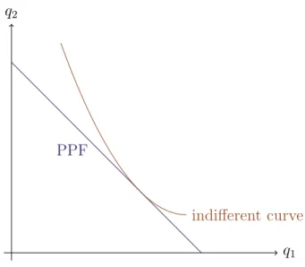
The set of nonnegative output pair (q1, q2) that can be produced using the labor inputs available is known as the production possibility set, which is given by
a1q1+ a2q2 ≤ ¯L. (20)
Production possibility frontier (PPF) is the set represented in (20) with equality.
The slope of PPF is a measure of how much the output of good j can increase if the country decreases the output of good i by one marginal unit. In other words, the slope represents the opportunity cost to produce good i in terms of good j. The slope is also related to the definition of comparative advantage. A country has a comparative advantage in producing good i if the opportunity cost is lower in that country than it is in other countries.
2.1.2 Consumption
Let xi denote the consumption of good i, and U : R2 7→ R be the utility function assumed to be strictly quasi-concave. Consider the utility maximizing problem of a representative household who inelastically supplies ¯L units of labor:
maxx1,x2 U (x1, x2) (21)
q1 q2
PPF
indifferent curve
Figure 1: Production possibility set under autarky. subject to
x1+ px2 ≤ w ¯L. (22)
It yields the demand functions for the goods.
By imposing the market-clearing condition under the autarky, xi = qi, the budget set (22) coincides with the production possibility set (20). (See again Figure 1.)
2.1.3 Free trade equilibrium
In the autarkic environments, the goods markets must clear separately in each country. In contrast, the market clearing for goods under free trade requires qi+ qi∗ = xi+ x∗i.
Assume that a1/a2 < a∗1/a∗2. In other words, Home has a comparative advantage in producing good 1. Then p > p∗ in the autarky equilibrium. If the relative price in free trade equilibrium, denoted by ˆp, satisfies
a2/a1 > ˆp > a∗2/a∗1, (23) Home is fully specialized in good 1 while Foreign is specialized in good 2.3 Therefore, the supplies of the goods are independent of the relative prices: q1+q1∗ = ¯L/a1 and q2+q∗2 = ¯L∗/a∗2. If the relative price satisfying the market clearing condition follows Eq.(23), then that is an equilibrium with free trade.
3Since a2/a1 > ˆp, we have (1 − wa1)/a1> (ˆp − wa2)/a2. That is, given ˆp, a marginal increase in input to produce good 1 generates a greater profit than that to produce good 2 at Home (we still normalize the price of good 1 to one under free trade).
2.2 gains from trade
For a given ˆp and w, competitive production leads to a revenue maximization: max[(1/a1)L1+ (ˆp/a2)L2] = (1/a1− w) ¯L. The zero-profit condition implies the income of households in Home is w ¯L = 1/a1, in which the income is also maximized. Thus, free trade can be no worse than autarky (see Figure 3).
As an extreme case, the free trade prices may equal to the autarky prices. If so, there is no gains from trade. Otherwise, the levels of (indirect) utility strictly increase in both the countries.
q1 q2
PPF (closed)
q1 PPF (open)
indiff. (closed) indiff. (open)
x1
Figure 2: PPF changes.
2.3 2 countries, many goods, 1 factor
Dornbusch, Fischer and Samuelson (1977) provide an important generalization of the Ricard model—a continuum of tradeable goods. Dornbusch, Fischer and Samuelson (1980) discuss the case of two factors as Heckscher-Ohlin model. The framework is also employed by many fields, including Matsuyama (2000, 2007), Eaton and Kortum (2002), Grossman and Rossi-Hansberg (2010), and Naito (2012).
2.3.1 Production
Consider there is a continuum of competitive industries, indexed by z ∈ [0, 1], each producing a homogeneous good, also indexed z. Let a(z) be the unit labor requirement of good z at Home. Define relative labor requirement as follows
A(z) = a
∗(z)
a(z) . (24)
Without loss of generality, we assume A′(z) < 0. In other words, Home has comparative advantages in low-indexed goods.
The autarky prices are p(z) = wa(z) at Home. Under free trade, the law of one price holds: p(z) = p∗(z) = min{wa(z), w∗a∗(z)}. Thus, for a given relative wage w/w∗, we can define the threshold in z by
w
w∗ = A(ˆz), (25)
such that Home produces only goods in [0, ˆz], whereas Foreign produces only goods in [ˆz, 1]. This equation determines the threshold ˆz inversely by w/w∗. The prices become
p(z) = p∗(z) = wa(z), for z ∈ [0, ˆz], (26) p(z) = p∗(z) = w∗a∗(z), for z ∈ [ˆz, 1]. (27)
2.3.2 Consumption
Assume that households have the Cobb-Douglas utility defined over z as U =
∫ 1
0
ln x(z)dz. (28)
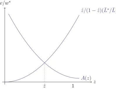
The Home income, wL, must equal the world expenditure on Home goods, ˆz(w ¯L + w∗L¯∗). This condition yields
w w∗ =
ˆ z 1 − ˆz
L¯∗
L¯ (29)
Eqs. (24) and (29) derives the relative wage and the patterns of trade in equilibrium (see Figure 3).
Consider, for exmaple, that technological progress in Home decreases ai for all i. Then the locus of A(z) shifts upward, by which the relative wage rises and Home specializes in the expanded range of goods.
Problem 2.1. Using (31), examine whether the countries can be better off by technological change.
z w/w∗
A(z) ˆ
z/(1 − ˆz)( ¯L∗/ ¯L)
ˆ
z 1
Figure 3: The equilibrium relative wages and patterns of specialization. 2.3.3 gains from trade
The indirect utility of Home residents is U = ∫01ln[w/p(z)]dz. Under autarky,
U = −
∫ 1
0
ln a(z)dz, (30)
and under free trade,
U = −
∫ zˆ 0
ln a(z)dz +
∫ 1
zˆ
ln
[ w
w∗a∗(z) ]
dz. (31)
The gains from trade, which are a difference in the indirect utilities, are
∫ 1
zˆ
ln[ A(ˆz) A(z) ]
dz > 0. (32)
Similarly, Foreign can also benefit from free trade.
3 The Heckscher-Ohlin Model (KOM, ch5)
point Changes in prices and production occur with the reallocation of factors.
3.1 2 countries, 2 goods, 2 factor
The Heckscher-Ohlin model is a landmark study changing our view on the international trade. The Heckscher-Ohlin model shows there are gains from trade even if the countries have identical technology. This is a complement of the Ricardian model finding that a source of comparative advantage comes from the difference in (labor) productivity.
The model is a full-fledged general equilibrium model allowing us to examine interrelashions among countries, factors, and industries. The Heckscher-Ohlin model derives four famous theorem, all of which imply the partial equilibrium thinking can be misleading.
1. Heckscher-Ohlin theorem A country will export that commodity which intensively uses its abundant factor.
2. Factor price equalization (FPE) Countries that produce the same mix of products with the same product prices and the same technologies have the same factor prices, regardless of their factor endowments.
3. Rybczynski theorem An increase in the endowment of labor causes a more than pro- portionate increase in output of the labor intensive god and a reduction in the output of the capital-intensive good.
4. Stolper-Samuelson theorem An increase in the relative price of the labor intensive good leads to a rise in the relative as well as the real return of labor and a decline in the relative and real return to capital.
The standard Heckscher-Ohlin model has the following features:
• Supply. There is two factors of production, e.g., labor and capital, whose endowments are exogenously given. There are two goods produced by constant returns to scale technology in perfectly competitive markets.
• Demand. There is no specific assumption. Trade account should be balanced.
• Geography. The goods can be traded without transport costs. The factors of production are freely mobile between the industries but immobile between the countries.
By introducing capital, the Heckscher-Ohlin model can describe the rich behavior of realloca- tion between sectors.
There are numerous extensions and empirical tests of the Heckscher-Ohlin models. Quah (2007) and Costinot (2009) develop a generalization of the model by using supermodular programming. Oniki and Uzawa (1965), Nishimura and Shimomura (2002), and Bajona and Kehoe (2010) examine a dynamic Heckshcer-Ohlin model. Trefler (1995) discusses the empirical performance of Heckscher-Ohlin theorem.
3.2 equilibrium
The section follows Leamer (1995). As in the Recardian model, the equilibrium is charac- terized by resource constraints and zero-profit conditions.
Let aiL and aiK be the units of labor and capital required to produce good i, respectively. We assume both are constant for simplicity.
The zero profit condition implies
a1Lw + a1Kr ≥ 1, (33)
a2Lw + a2Kr ≥ p, (34)
where r is return to capital. If w > 0 and r > 0, then the equality holds. In matrix form,
A′w ≥ p, w ≥ 0, (35)
where
A =
a1L a2L
a1K a2K
, w = (w, r)′ and p = (1, p)′.
From (35), when factor prices are strictly positive, w = p(A′)−1. If there exists an inverse matrix of A′, the factor prices w is uniquely determined. Under free trade, countries face the same price vector p. If the countries have the same technology, then they must have the same factor prices. That’s FPE.
Note that the levels of factor prices are independent of factor supplies. Thus, migration has no impact on wage, or capital accumulation has no impact on return to capital, ceteris paribus. Crudely, if technology and knowledge diffuse to developing countries and trade becomes freer, then the differences in factor prices between developed and developing countries will disappear.
Definition 3.1. Sector i is a capital-intensive sector if aiK
aiL
> ajK ajL
. (36)
for j ̸= i. In this case, sector j is labor-intensive. Problem 3.1. Prove Stolper-Samuelson theorem.
Stolper-Samuelson theorem implies that a change in the relative price creates conflicts in interests. A higher relative price of capital-intensive goods leads to a lower wage-rental ratio (w/r). If we interpret capital as high skilled labor to create high-tech products, it may help us to understand the rising inequality of wages in the developed countries.4
The resource constraint at Home is
a1Lq1+ a2Lq2 ≤ ¯L, (37)
a1Kq1+ a2Kq2 ≤ ¯K, (38)
In matrix form,
Aq ≤ v, q ≥ 0, (39)
where q = (q1, q2)′ and v = ( ¯L, ¯K)′.
Problem 3.2. Prove Rybczynski theorem.
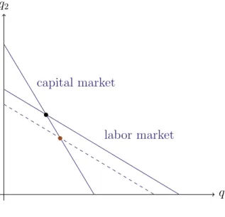
We demonstrate the theorem graphically. Assume that sector 1 is capital intensive. Figure 4 depicts the production possibility frontier given by Eqs. (37) and (38). If both factors of production are full employed, equilibrium output is at the intersection of the two lines.
Taking immigration as an example, consider an increase in ¯L. The consequence is shown as in Figure 5. Partial equilibrium model of the labor market may conjecture a decline of
4Despite the obvious relevance of trade in explaining the income distribution, the magnitude and implication are still debated. See, for example, Krugman (2008), Gancia and Zilibotti (2009), and 櫻井 (2014). The empirical literature is summarized by Deardorff (1984) and Baldwin (2008).
q1 q2
labor market capital market
Figure 4: Production possibility set.
wage rates. However, since the prices of goods are fixed, the wage is also fixed as a result of FPE. FPE occurs if labor demand also increases. The key to understand is reallocation of capital. In pursuit of profit opportunities created by lower wage, capital moves toward the labor-intensive sector, and hence it creates labor demand to completely eliminate the partial equilibrium impacts on wages.
q1 q2
capital market
labor market
Figure 5: Relaxing the labor constraint.
Finally, we shortly see the direction of trade. In autarky, the goods markets must clear domestically, and thus the equilibrium consumption is at the kinked point of the PPF. Assume again good 1 is capital intensive (or, good 2 is labor intensive) and the countries have the
same technology A. Given homothetic preference, the relative price p in autarky equilibrium is higher in a country having lower endowment ratio ¯L/ ¯K because of fewer relative supplies of the labor intensive goods. Free trade price lays between the autarkic price of both countries if both goods are produced. The change in relative price readily confirms the Heckscher-Ohlin theorem. In this case trade does not affect the production bundle due to the assumption of constant unit costs.
Anderson, J.E. (2011) “The gravity model,” Annual Review of Economics 3, 133–160.
Anderson, J.E. and E. Van Wincoop (2003) “Gravity with gravitas: a solution to the border puzzle,” American Economics Review 42, 691–751.
Bajona, C. and T. J. Kehoe (2010) Trade, growth, and convergence in a dynamic Heckscher- Ohlin Model,” Review of Economic Dynamics 13, 487–513.
Baldwin, R. E. (2008) The Development and Testing of Heckscher-Ohlin Trade Models: A Review,” The MIT Press.
Bertoli S. and J. Fern´andez-Huertas Moraga (2013) “Multilateral resistance to migration,” Journal of Development Economics 102, 79–100.
Bosker, E.M. and H. Garretsen (2010) “Trade costs, market access, and economic geography: Why the empirical specification of trade costs matters,” in van Bergeijk and Brakman,
“The Gravity Model in International Trade: Advances and Applications,” Cambridge Univ Press.
Brainard, S.L. (1997) “An Empirical Assessment of the Proximity-Concentration Trade-off Between MultinationalSales and Trade,” American Economics Review 87, 520–544. Costinot, A. (2009) “AN ELEMENTARY THEORY OF COMPARATIVE ADVANTAGE,”
Econometrica 77, 1165–1192.
Deardorff, A. (1984) “Testing Trade Theories and Predicting Trade Flows,” in R.W. Jones and P.B. Kenen, “Handbook of International Economics, volume 2” Amsterdam: North- Holland, pp.467–517.
Dornbusch, R., S., Fischer and P. Samuelson (1977) “Comparative advantage, trade and pay- ments in a Ricardian model with a continuum of goods,” American Economics Review 67, 823–839.
Dornbusch, R., S., Fischer and P. Samuelson (1980) “Heckscher-Ohlin trade theory with a continuum of goods,” Quarterly Journal of Economics 95, 203–224.
Eaton, J. and S. Kortum (2002) “Technology, geography and trade,” Econometrica 70, 1741– 1779.
Gancia, G. and F. Zilibotti (2009) “Technological change and the wealth of nations,” Annual Review of Economics 1, 93–120.
Grossman, G.M. and E. Rossi-Hansberg (2010) “External Economies and International Trade Redux,” Quarterly Journal of Economics 125, 829–858.
Head, Keith and Thierry Mayer (2014) “Gravity Equations: Workhorse, Toolkit, and Cook- book,” Handbook of International Economics (vol.4)”, eds. Gopinath, Helpman, and Rogoff.
Keller, W. and S.R. Yeaple (2013) “The gravity of knowledge,” American Economics Review 103, 1414–1444.
Kleinert, J. and F. Toubal (2010) “Gravity for FDI,” Review of International Economics 18, 1–13.
Krugman, P.R. (2008) “Trade and wages, reconsidered,” Brookings Papers on Economic Activ- ity Spring 2008, 103–154.
Leamer, E.E. (1995) “The Heckscher-Ohlin model in theory and practice,” Graham Lecture, Princeton Studies in International Finance 77, Princeton University.
Matsuyama, K. (2000) “A Ricardian Model with a Continuum of Goods under Nonhomothetic Preferences: Demand Complementarities, Income Distribution, and North‐ South Trade,” Journal of Political Economy 108, 1093–1120.
Matsuyama, K. (2007) “Beyond Icebergs: Towards a Theory of Biased Globalization,” Review of Economic Studies 74, 237–253.
Naito, T. (2012) “A Ricardian model of trade and growth with endogenous trade status ,” Journal of International Economics 87, 80–88.
Nishimura, K. and K. Shimomura (2002) “Trade and Indeterminacy in a Dynamic General Equilibrium Model,” Journal of Economic Theory 105, 244–260.
Obstfeld, M. and K. Rogoff (2001) “The Six Major Puzzles in International Macroeconomics: Is There a Common Cause?” NBER Macroeconomics Annual 2000, Volume 15, ed. B. S. Bernanke and K. Rogoff, The MIT Press.
Okawa, Y. and E. Van Wincoop (2012) “Gravity in international finance,” Journal of Inter- national Economics 87, 205–215.
Oniki, H. and H. Uzawa (1965) “Patterns of Trade and Investment in a Dynamic Model of International Trade,” Review of Economic Studies 32, 15–38.
Quah, J. K.-H. (2007) “THE COMPARATIVE STATICS OF CONSTRAINED OPTIMIZA- TION PROBLEMS,” Econometrica 75, 401–431.
櫻井宏二郎 (2014) 『グローバル化と日本の労働市場—貿易が賃金格差に与える影響を中心に』 日本銀行ワーキングペーパーシリーズ, 14–j–5.
Trefler, D. (1995) “The Case of the Missing Trade and Other Mysteries,” American Economics Review 85, 1029–1046.
Waugh, M.E. (2010) “International Trade and Income Differences,” American Economic Re- view 100, 2093–2124.