2D Partitioning Based Graph Search for the Graph500 Benchmark
Koji Ueno
Tokyo Institute of Technology / JST CREST [email protected]
Toyotaro Suzumura Tokyo Institute of Technology IBM Research – Tokyo / JST CREST
Abstract—Graph500 is a new benchmark to rank supercompu- ters with a large-scale graph search problem. We found that the provided reference implementations are not scalable in a large distributed environment. In this paper we implement an optimized method based on 2D based partitioning. Our implementation can solve BFS (Breadth First Search) of large- scale graph with 68.7 billion vertices and 1.1 trillion edges for 24.12 seconds with 512 nodes and 12288 CPU cores. This record corresponds to 22.8 GE/s. We found 2D based partition- ing method is scalable for large-scale distributed systems. We also demonstrate thorough study of performance characteris- tics of our optimized implementation and reference implementations in a large-scale distributed memory super- computer with a Fat-Tree based Infiniband network.
Keywords-component: Graph500, BFS, Supercomputer
I. INTRODUCTION
Large-scale graph analysis is a hot topic for various fields of study, such as social networks, micro-blogs, protein- protein interactions, and the connectivity of the Web. The numbers of vertices in the analyzed graph networks have grown from billions to tens of billions and the edges have grown from tens of billions to hundreds of billions. Since 1994, the best known de facto ranking of the world’s fastest computers is TOP500, which is based on a high performance Linpack benchmark for linear equations. As an alternative to Linpack, Graph500 [1] was recently developed. We con- ducted a thorough study of the algorithms of the reference implementations and their performance in an earlier paper [18]. Based on that work, we now propose a scalable and high-performance implementation of an optimized Graph500 benchmark for large distributed environments. Here are the main contributions of our new work:
1. Proposal of efficient implementation of parallel level- synchronized BFS (Breadth-First Search) with 2D graph partitioning.
2. Optimization of the complete flow of the Graph500 as a lighter-weight benchmark with better graph generation and validation.
3. A thorough study of the performance characteristics of our implementation and those of the reference imple- mentations.
Here is the organization of our paper. In Section II, we give an overview of Graph500 and parallel BFS algorithms. In Section III, we describe the scalability problems of the reference implementations. We explain the efficient imple- mentation in Section IV, and the optimized implementation of the Graph500 benchmark in Section V. In Section VI, we
describe our performance evaluation and give detailed profiles from our optimized method running on the Tsubame 2.0 supercomputer. We review related work in Section VII, and conclude and consider future work in Section VIII.
II. GRAPH500 AND PARALLEL BFSALGORITHMS In this section, we give an overview of the Graph500 benchmark [1], the parallel level-synchronized BFS method, and then the adaptation of this method to distributed compu- ting.
A. Graph500 Benchmark
In contrast to the computation-intensive benchmark used by TOP500, Graph500 is a data-intensive benchmark. It does breadth-first searches in undirected large graphs generated by a scalable data generator based on a Kronecker graph [16]. The benchmark has two kernels: Kernel 1 constructs an undirected graph from the graph generator in a format usable by Kernel 2. The first kernel transforms the edge tuples (pairs of start and end vertices) to efficient data structures with sparse matrix formats, such as CSR (Compressed Sparse Row) or CSC (Compressed Sparse Column). Then Kernel 2 does a breadth-first search of the graph from a randomly chosen source vertex in the graph.
The benchmark uses the elapsed times for both kernels, but the rankings for Graph500 are determined by how large the problem is and by the throughput in TEPS (Traversed Edges Per Second). This means that the ranking results basically depend on the time consumed by the second kernel.
After both kernels have finished, there is a validation phase to check if the result is correct. When the amount of data is extremely large, it becomes difficult to show that the resulting breadth-first tree matches the reference result. Therefore the validation phase uses 5 validation rules. For example, the first rule is that the BFS graph is a tree and does not contain any cycles.
There are six problem sizes: toy, mini, small, medium, large, and huge. Each problem solves a different size graph defined by a Scale parameter, which is the base 2 logarithm of the number of vertices. For example, the level Scale 26 for toy means 226 and corresponds to 1010 bytes occupying 17 GB of memory. The six Scale values are 26, 29, 32, 36, 39, and 42 for the six classes. The largest problem, huge (Scale 42), needs to handle around 1.1 PB of memory. As of this writing, Scale 38 is the largest that has been solved by a top- ranked supercomputer.
B. Level-synchronized BFS
All of the MPI reference implementation algorithms of the Graph500 benchmark use a “level-synchronized breadth-first
search”, which means that all of the vertices at a given level of the BFS tree will be processed (potentially in parallel) before any vertices from a lower level in the tree are processed. The details of the level-synchronized BFS are explained in [2][3].
Algorithm I: Level-synchronized BFS
1 for all vertices v in parallel do 2 | PRED[v]← -1;
3 | VISITED [v] ← 0; 4 PRED [r] ← 0 5 VISITED[r] ← 1 6 Enqueue(CQ, r) 7 While CQ != Empty do 8 | NQ ← empty
9 | for all u in CQ in parallel do 10 | | u ← Dequeue(CQ)
11 | | for each v adjacent to u in parallel do 12 | | | if VISITED [v] = 0 then 13 | | | | VISITED [v] ← 1; 14 | | | | PRED [v] ← u; 15 | | | | Enqueue(NQ, v) 16 | swap(CQ, NQ);
Algorithm I is the abstract pseudocode for the algorithm that implements level-synchronized BFS. Each MPI process has two queues, CQ (Current Queue) and NQ (Next Queue), and two arrays, PRED for a predecessor array and VISITED to track whether or not each vertex has been visited.
We start BFS from the vertex r. At any given time, CQ is the set of vertices that must be visited at the current level. At level 1, CQ will contain the neighbors of r, so at level 2, it will contain their pending neighbors (the neighboring vertices that have not been visited at levels 0 or 1). The algorithm also maintains NQ, containing the vertices that should be visited at the next level. After visiting all of the nodes at each level, the queues CQ and NQ are swapped at line 16.
VISITED is a bitmap that represents each vertex with one bit. Each bit of VISITED is 1 if the corresponding vertex has been already visited and 0 if not. PRED has a predecessor vertex for each vertex. If an unvisited vertex v is found at line 12, the vertex u is the predecessor vertex of the vertex v at line 14. When we complete BFS, PRED forms a BFS tree, the output of kernel2 in the Graph500 benchmark.
At each level, the set of all vertices v is the NQ nominee, now called “NQ-N”. NQ-N has all the adjacent vertices of the vertices in CQ that would be potentially stored in NQ. NQ-N is obtained from line 9 to line 11 in the algorithm.
The Graph500 benchmark provides 4 different reference implementations based on this level-synchronized BFS method. Their details and algorithms appear in an earlier paper [18]. However we found out that the fundamental concept of the level synchronized BFS can be viewed as a sparse-matrix vector multiplication. With reference to the detailed algorithmic explanations in [18], we only explain the basic BFS method here.
C. Representing Level-Synchronized BFS as Sparse- Matrix Vector Multiplication
The level-synchronized BFS in II-B is analogous to a Sparse-Matrix Vector multiplication (SpMV) [19] which is computed as y = Ax where x and y are vectors and A is a sparse matrix.
A is an adjacency matrix for a graph. Each element of this matrix is 1 if the corresponding edge exists and 0 if not. The vector x corresponds to CQ (Current Queue) where x(v) = 1 if the vertex v is contained in CQ and x(v) = 0 if not. Then NQ-N, the NQ nominees, can be represented as the elements corresponding to the vertexes in v whose values are greater than 0 in the vector y. However, the BFS method requires the computations from Lines 12 to 15 in its algorithm.
D. Mapping Reference Implementations to SpMV
In a distributed memory environment, the graph data and vertex data must be distributed. There are four MPI-based reference implementation of Graph500: replicated-csr (R- CSR), replicated-csc (R-CSC), simple (SIM), and one_sided (ONE-SIDED).
Assume that we have a total of P processors, and all four of the reference implementations simply divide PRED and NQ into P blocks and each processor handles one block. Figure 1 shows how SpMV can be computed in parallel with P processors. There are two partitioning methods for the sparse matrix, vertical partitioning that divides it into P divisions in vertically (left), and horizontal partitioning that divides the matrix horizontally (right) into P divisions. The computation of the reference implementations can be abstracted as the computation of SpMV. R-CSR and R-CSC use vertical partitioning for SpMV while SIM and ONE- SIDED use horizontal partitioning for SpMV.
,
Figure 1. SpMV with vertical and horizontal partitioning III. SCALABILITYISSUESOFREFERENCE
IMPLEMENTATIONS
In this section we give overviews of three reference im- plementations of Graph500, R-CSR (replicatedc-csr), R- CSC (replicated-csc), and SIM (simple) and we use experi- ments and quantitative data to show why none of these algorithms can scale well in large systems.
Before moving to the detailed descriptions of each imple- mentation, we need to cover how CQ (Current Queue) is implemented in the reference implementations. The refer- ence implementations also use bitmaps with one bit for each vertex in CQ and NQ. In these bitmaps, if a certain vertex v is in a queue (CQ or NQ), then the bit that corresponds to that vertex v is 1 and if not, then the bit is 0.
We categorize the reference implementations into replica- tion-based and non-replicated methods, which are described in Sections III-A and III-B.
A. Replication-based method 1) Algorithm Description:
For the R-CSR and R-CSC methods that divide an adja- cency matrix vertically, CQ must be duplicated to all of the processes. Each process independently computes part of NQ- N. From the NQ-N vertices, each process computes only NQ for its own portion.
Copying CQ to all of the other processes means the distri- buted NQ must be sent to all of the other processes. CQ (and NQ) is represented as a relatively small bitmap. For relative- ly small problems with limited amounts of distribution, the amounts of data are reasonable and this method is effective.
However, since the size of CQ is proportional to the num- ber of vertices in the entire graph, the data volume sent to each process is increasing in the same proportion. This copying operation leads to a large amount of communication in a large system with many transmissions.
2) Quantitative Evaluation for Scalability:
Figure 2 shows the communication data volume for each node with the replication-based implementation and SCALE of 26 for each node as the problem size. This is a weak- scaling version, and computes the theoretical results when using 2 processes per node. In such a weak-scaling setting, the number of vertices increases in proportion to the increas- ing number of nodes. This result clearly shows that the replication-based method is not scalable for a large environ- ment.
Figure 2. Theoretical message size per node (GB) B. Non-replicated Method
1) Algorithm Description:
The simple reference implementation or SIM that divides an adjacent matrix in a horizontal fashion, locates the portion of the CQ by dividing it into P. The NQ queue is already divided into P blocks, and so the NQ queue from the previous level can be used as the vector x.
Each process retrieves NQ Nominees (NQ-N) from the divided CQ and the partial adjacency matrix owned by the process. These NQ-N entries include both the vertices to be handled by the local process and by other processes. By using NQ-N, PRED and NQ are updated. The local vertices
are handled by local processes, but the vertices for other processes are transmitted to those vertices.
The number of the NQ-N vertices to be transmitted to remote processes can be up to the number of edges of the adjacency matrix owned by the sender-side process. Thus the communication data volume is constant without regard to the number of nodes. More precisely, the communication data volume can be smaller as the number of nodes decreases because the number of vertices to be processed locally becomes larger when there are fewer nodes in total. Howev- er, in some cases the communication data volume remains constant without regard to the number of nodes, because the number of local vertices can become negligibly small if the total number of nodes is sufficiently large.
However, the replication-based method with vertical partitioning transmits CQ as a bitmap. However in the simple implementation, SIM needs to send pairs of a CQ vertex and an NQ-N (Next Queue nominees) vertex because the predecessor vertex is needed to update PRED, the predeces- sor array. Therefore, the replication-based approach with vertical partitioning is better than the simple approach in a small-scale environment with fewer nodes.
2) Quantitative Evaluation for Scalability
The other two reference implementations with horizontal partitioning are called “simple” and “one_sided” and they have no problems with the amount of communicated data, just like the replication-based method. However, all-to-all communication that sends a different data set to each of the other nodes is needed when sending the NQ-N vertices. This all-to-all communication is not scalable for large distributed- memory environments.
Figure 3. Average data rate per node with all-to-all communication
Figure 3 shows the communication speed of the all-to-all communication on Tsubame 2.0 when using 4 MPI processes per node. We used MVAPICH2 1.6 as the MPI implementation. The communication was implemented with the MPI_Alltoall function, and we used three different transmission buffer sizes, 64 MB, 256 MB, and 1,024 MB.
The amount of data that each node transmits to other nodes is 4 MB when using the 1,024 MB buffer size, 64 nodes, and 256 MPI processes. The results shown in Figure 3 show that the all-to-all communication is not scalable.
The main reason of performance degradation is communi- cation latency. With 512 nodes, the performance is quite slow with a small buffer size such as 64 MB. Also, even if
we use 1,024 MB as the buffer size, the performance is 1/4 of 32 nodes.
Our experimental testbed, TSUBAME 2.0, uses a Fat-Tree structure with its Infiniband network. If the theoretical peak performance were achieved, there would be no performance degradation even for all-to-all communication is among all of the nodes. However, the communication latency cannot be ignored in a large system. The actual performance is always less than the theoretical maximum.
IV. SCALABLE APPROACH
To solve the scalability problems described in Section III, we adapt the 2D partitioning method. In this section, we describe the algorithm of 2D partitioning-Based BFS and our efficient implementation.
A. 2D Partitioning-Based BFS
The 2D Partitioning-Based parallel breadth-first search algorithm was proposed in [4]. Their algorithm is also based on a level-synchronized BFS but it uses 2D partitioning technique to reduce the communication costs. The concept of 2D partitioning is a mixture of two 1D partitioning types, vertical and horizontal partitioning. Here is a brief overview of the 2D partitioning technique.
Assume that we have a total of
P
processors, where theC
R
P = ×
processors are logically deployed in a two dimensional mesh which hasR
rows and C columns. Adjacency matrix is divided as shown in Figure 4 and the processor( j i , )
is responsible for handling the C blocks fromA
i(, j1) toA
i(,Cj). The vertices are divided intoR × C
blocks and the processor
( j i , )
handles the k-th block, where k is computed as( j − ) 1 × R + i
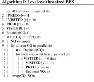
.Each level of the level-synchronized BFS method with 2D partitioning is done in 2 communication phases called
“expand” and “fold”. In the expand phase, every processor copies its CQ to all of the other processors that exist in the same column, similar to vertical 1D partitioning. In the fold phase, each processor receives the edges from the other processors that exist in the same row, similar to horizontal 1D partitioning. Therefore, this is equivalent to a method of combining the two types of 1D partitioning. If C is 1, this corresponds to the vertical 1D partitioning and if R is 1, it corresponds to the horizontal 1D partitioning.
In each fold phase, it first searches all of the adjacent vertices against each vertex v from CQ obtained in the expand phase, and then sends a tuple of (v, u), where u is one of the discovered adjacent vertices, to the corresponding processor where v is located.
The advantage of 2D partitioning is to reduce the number of processors that need to communicate. Both types of 1D partitioning require all-to-all communication. However, the 2D partitioning can reduce the number of communicating processors for better scalability in large computing environ- ments, since the expand phase only requires communication among the nodes in the same column and the fold phase only
requires communication among the processors in the same row.
Figure 4. 2D Partitioning Based BFS [4] B. Implementation
We now explain our efficient implementation of the level- synchronized BFS with 2D partitioning. As described in Section III-C, the processors are deployed in an
R × C
mesh and
P
is the number of processors.The communication method of the expand phase is the same approach as R-CSC. Each set of vertices in CQ is represented as a bitmap and all of the processors gather CQ at each level by using the MPI_AllGather function. We divide the processing task of the fold phase into senders and receivers. The senders send the edges. The receivers receive edges from the senders and update VISITED, PRED, and NQ.
Algorithm II: Optimized 2D partitioning algorithm 1 for all vertexes lu in NQ do
2 | NQ[lu] ← 0 3 NQ [root] ← 1 4 fork; 5 for level = 1 to
6 | CQ ← all gather NQ in this processor-column; 7 | parallel Sender Processing and Receiver Processing 8 | Synchronize;
9 | if NQ = for all processors then 10 | | terminate loop;
11 join;
Sender Processing
1 for all vertexes gu in CQ parallel do (contiguous access) 2 | if CQ [gu] = 1 then
3 | for each local vertex v adjacent to gu do
4 | | send tuple (gu, v) to the processor which owns vertex v
Receiver Processing
1 for each received tuple (gu, v) parallel do 2 | if visited[v] = 0 then
3 | | PRED[v] ← gu; 4 | | VISITED[v] ← 1; 5 | | NQ [v] ← 1;
The algorithm appears as Algorithm II. In Lines 1-2, NQ is initialized and the BFS root is inserted into NQ in line 3.
Lines 5-10 are done by all of the processors. Line 6 is the expand communication. In Line 7, Sender Processing and Receiver Processing run in parallel.
The Sender Processing and Receiver Processing are han- dled by multiple parallel threads. Our implementation uses hybrid parallelism of MPI and OpenMP for communication and computational efficiency. The communications between these two processing are done asynchronously. Our imple- mentation has highly efficient processing with this parallel and asynchronous communication.
V. OPTIMIZING GRAPH GENERATION AND VALIDATION
We also propose a method to improve the Graph500 benchmark for lightweight experiments with better fault tolerance. The basic optimization idea for the generation phase is to avoid generating the same data as the reference implementations.
The current Graph500 benchmark must conduct 64 itera- tions of the BFS executions and validations. To shorten each experimental cycle, our implementation also optimizes the validation phase by distributing the edge tuples to all of the processors in the time between the construction phase and the first BFS execution.
A. Graph Generation
When selecting the start vertex of BFS, we must select a vertex that has more than one edge. Thus we need a bitmap has_edge to track whether a vertex has more than one edge. This bitmap represents each vertex with one bit, so if the problem size is large, the bitmap has_edge cannot be stored in one processor. However, if we simply divide the has_edge bitmap among the P processors, there is non-scaling all-to-all communication among the processors.
For this reason, the reference implementation allocates processors with a 2D mesh of R x C. The has_edge bitmap is divided into C blocks from
H
1 toH
C . The processor)
,
( j i
is allocated to theH
j block. This division method indicates that the R processors in the j-th processor column have the sameH
j blocks, and each of the C processors at the i-th processor row has different blocks.Processors in the same processor column generate differ- ent portions of the graph data set. Each processor in the same processor row generates exactly the same data, and only the edges that are generated locally affect the has_edge bitmap. This generation method is optimized by avoiding the communication of edge data.
However, the R processors in each row redundantly gener- ate the same portion of the graph data set. Increasing the number of distributions with the weak-scaling setting is not scalable. For this reason, we further modified the generation method in a way that each processor in the same row generates a different portion of the data set, and transmits the edge data to update the has_edge bitmap.
B. Validation
The validation phase dominates the overall time of the Graph500 benchmark, and so it is critically important to accelerate this phase to speed up the entire experiment. The validation determines the correctness of the BFS result based on the edge tuples generated in the graph generation phase. By profiling the validation phase of the reference implemen- tation, we found two validation rules in the Graph500 specification dominating the all-to-all communications. 1) Each edge in the input list has vertices with levels that
differ by at most one or neither is in the BFS tree
2) Each node and its parent are joined by an edge in the original graph.
A processor that owns an edge tuple (v0, v1) needs to communicate with the owner processor of v0 and the owner processor of v1. Implemented in a naïve fashion, this requires all-to-all communication involving all of the processors, which is not scalable. We devised an approach that divides the edge tuples with 2D partitioning and allocates them to each processor before the validation phase. The number of processors involved in communication is fewer than the original version, making the work scalable.
VI. PERFORMANCE EVALUATION
We used Tsubame 2.0, the fifth fastest supercomputer in the TOP500 list of June 2011, to evaluate the scalability of our optimized implementation.
A. Overview of the Tsubame 2.0 supercomputer
Tsubame 2.0 [15] is a production supercomputer operated by the Global Scientific Information and Computing Center (GSIC) at the Tokyo Institute of Technology. Tsubame 2.0 has more than 1,400 compute nodes interconnected by high- bandwidth full-bisection-wide Infiniband fat nodes.
Each Tsubame 2.0 node has two Intel Westmere EP 2.93 GHz processors (Xeon X5670, 256-KB L2 cache, 12-MB L3), three NVIDIA Fermi M2050 GPUs, and 50 GB of local memory. The operating system is SUSE Linux Enterprise 11. Each node has a theoretical peak of 1.7 teraflops (TFLOPS). The main system consists of 1,408 computing nodes, and the total peak performance can reach 2.4 PFLOPS. Each of the CPUs in Tsubame 2.0 has six physical cores and supports up to 12 hardware threads with Intel’s hyper-threading technol- ogy, thus achieving up to 76 gigaflops (GFLOPS).
The interconnect that links the 1,400 computing nodes with storage is the latest QDR Infiniband (IB) network, which has 40 Gbps of bandwidth per link. Each computing node is connected to two IB links, so the communication bandwidth for the node is about 80 times larger than a fast LAN (1 Gbps). Not only the link speed at the endpoint nodes, but the network topology of the entire system heavily affects the performance for large computations. Tsubame 2.0 uses a full-bisection fat-tree topology, which handles applications that need more bandwidth than provided by such topologies as a torus or mesh.
B. Evaluation Method
In the software environment we used gcc 4.3.4 (OpenMP 2.5) and MVAPICH2 [17] version 1.6 with a maximum 512 nodes. Tsubame 2.0 is also characterized as a supercomputer with heterogeneous processors and a large number of GPUs, but we did not use those parts of the system. Each node of Tsubame 2.0 has 12 physical CPU cores and 24 virtual cores with SMT (Simultaneous Multithreading). Our implementa- tion treats 24 cores as a single node and the same number of processors is allocated to each MPI process.
In our experiments, the 2D-partitioning-based processor allocation R x C was per Table 1. R and C were determined with the policy of allocating division numbers as similarly as possible. The number of MPI processes should be a power of two and the value of R and C was determined by the MPI processes irrespective of the number of nodes.
# of MPI processes 1 2 4 8 16 32 64
R 1 1 2 2 4 4 8
C 1 2 2 4 4 8 8
# of MPI processes 128 256 512 1024 2048 4096
R 8 16 16 32 32 64
C 16 16 32 32 64 64
Table 1. The values of R and C with the # of MPI processes
C. Comparison with Reference Implementations
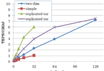
We compared U-BFS with the latest version (2.1.4) of the reference implementations in Figure 5 and Figure 6. This experiment was done in a weak-scaling fashion, so the problem size for each node was held constant, SCALE 26.
The horizontal axis is the number of nodes and the vertical axis is the performance for each node in ME/s.
U-BFS and the two reference implementations, R-CSR and R-CSC use 2 MPI processes for each node. The refer- ence implementation, simple, uses 16 MPI processes for each node, since the implementation does not use multithreading parallelism. As shown in the graph, there were some results that could not be measured due to problems in the reference implementations. When the number of nodes is increased for SIM, the system ran out of memory. With R-CSR and SCALE 32, a validation error occurred and there was a segmentation fault at higher SCALE values. With R-CSC, the construction phase crashes above SCALE 34. Our optimized implementation achieved 22.8 GEdges per second (TEPS) with 512 nodes (12,288 CPU cores) and SCALE 36. D. Comparison of Communication Data Volume
Figure 7 compares the communication data volume of our optimized method and the reference implementation in a weak-scaling setting. The vertical axis is the transmitted data volume (GB) per node involved in one traversal of BFS with the SCALE 26 problem size. This profiling used 2 MPI processes per node. The data volume of the replication-based reference implementations including R-CSC and R-CSR is a theoretical value since we could not measure the data with more than 256 nodes because of the limitations of the reference implementations. This graph shows the measured data for the 2D-partitioning-based methods.
The communication data volume of the replication-based reference implementations increases in proportion to the number of nodes for the weak-scaling setting since it needs Figure 5. Comparison with Reference
implementations (1~128 nodes) Figure 6. Comparison with Reference
implementations (1~512 nodes) Figure 7. Comparing Communication Data Volume
Figure 8. Performance comparison of the construction phase
Figure 9. Performance comparison of
the generation phase Figure 10. Performance comparison of the validation phase
to send CQ to all of the other processes. Meanwhile, the 2D- based partitioning method is scalable since the communica- tion data volume becomes relatively smaller with larger nodes.
E. Performance of Construction and Validation
Figure 8 compares the construction phases of our imple- mentation and the reference implementations in a weak- scaling setting. Our implementation finishes the construction phase twice as quickly compared to the reference implemen- tation.
Figure 9 shows the optimized generation method avoiding performance degradation above SCALE 33 where the reference implementations have problems.
Figure 10 compares our method with the reference im- plementation, where our method finishes the validation phase with less than one-third of the time of the original implementations.
VII. RELATED WORK
Yoo [4] presents a distributed BFS scheme that scales on the IBM BlueGene/L with 32,768 nodes. Their optimization differs in the scalable use of memory since they use 2D (edge) partitioning of the graph instead of conventional 1D (vertex) partitioning to reduce the communication overhead. Since BlueGene/L has a 3D torus network, they developed efficient collective communication functions for that network. Bader [3] describes the performance of optimized parallel BFS algorithms on multithreaded architectures such as the Cray MTA-2.
Agarwal [2] proposes an efficient and scalable BFS algo- rithm for commodity multicore processors such as the 8-core Intel Nehalem EX processor. With the 4-socket Nehalem EX (Xeon 7560, 2.26 GHz, 32 cores, 64 threads with Hyper- Threading), they ran 2.4 times faster than a Cray XMT with 128 processors when exploring a random graph with 64 million vertices and 512 million edges, and 5 times faster than 256 BlueGene/L processors on a graph with an average degree of 50. The performance impact of their proposed optimization algorithm was tested only on a single node, but it would be worthwhile to extend their proposed algorithm to larger machines with commodity multicore processors, which includes Tsubame 2.0.
Harish [10] devised a method of accelerating single-source shortest path problems with GPGPUs. Their GPGPU-based method solves the breadth-first search problem in approx- imately 1 second for 10 million vertices of a randomized graph where each vertex has 6 edges on average. However, the paper concluded that the GPGPU-method does not match the CPU-based implementation for scale-free graphs such as the road network of the 9th DIMACS implementation challenge, since the distribution of degrees follows a power law in which some vertices have much higher degrees than others. However since the top-ranked supercomputers in TOP500 have GPGPUs for compute-intensive applications, it would be worthwhile to pursue the optimization of Graph500 by exploiting GPGPUs.
VIII. CONCLUDING REMARKS AND FUTURE WORK In this paper we proposed an efficient implementation of the Graph500 benchmark in a large-scale distributed memory environment. The reference code samples provided by the Graph500 site were not scalable nor optimized for such a large environment. Our efficient implementation is based on the level-synchronized BFS with 2D partitioning and asynchronous communication. Our implementation does 22.8 GE/s as TEPS (Traversal Edges Per Second) with SCALE 36 and 512 nodes of Tsubame 2.0. We also propose approaches for optimizing the generation and validation phases, which can accelerate the overall benchmark. Many of our proposed approaches in this paper can also be effective for other supercomputers such as Cray and Blue- Gene. For future work we will show the effectiveness of our implementation in other large systems.
REFERENCES [1] Graph500 : http://www.graph500.org/
[2] Virat Agarwal et al., 2010. Scalable Graph Exploration on Multicore Processors. SC 2010
[3] David A. Bader et al., Designing Multithreaded Algorithms for Breadth-First Search and st-connectivity on the Cray MTA-2. ICPP 2006,
[4] Andy Yoo et al., A Scalable Distributed Parallel Breadth-First Search Algorithm on BlueGene/L. SC 2005.
[5] D.A. Bader et al., HPCS Scalable Synthetic Compact Applications #2 Graph Analysis (SSCA#2 v2.2 Specification), 5 September 2007. [6] D. Chakrabarti, Y. Zhan, and C. Faloutsos, R-MAT: A recursive
model for graph mining, SIAM Data Mining 2004.
[7] Bader, D., Cong et al., On the architectural requirements for efficient execution of graph algorithms. ICPP
[8] K. Madduri et al., ``Parallel Shortest Path Algorithms for Solving Large-Scale Instances,'' 9th DIMACS Implementation Challenge, 2006
[9] Richard C. Murphy et al., "DFS: A Simple to Write Yet Difficult to Execute Benchmark,", IISWC06
[10] Pawan Harish et al., Accelerating large graph algorithms on the GPU using CUDA. (HiPC'07),
[11] Daniele Paolo Scarpazza et al., Efficient Breadth-First Search on the Cell/BE Processor. IEEE Trans. Parallel Distrib. Syst. 2008
[12] Douglas Gregor et al., Lifting sequential graph algorithms for distributed-memory parallel computation. SIGPLAN 2005
[13] Grzegorz Malewicz et al,. Pregel: a system for large-scale graph processing. SIGMOD '10
[14] U. Kang et al., PEGASUS: A Peta-Scale Graph Mining System Implementation and Observations. ICDM '09
[15] Toshio Endo et al., Linpack Evaluation on a Supercomputer with Heterogeneous Accelerators. IPDPS 2010
[16] J. Leskovec, D. Chakrabarti, J. Kleinberg, and C. Faloutsos,
"Realistic, mathematically tractable graph generation and evolution, using kronecker multiplication," in Conf. on Principles and Practice of Knowledge Discovery in Databases, 2005.
[17] MVAPICH2: http://mvapich.cse.ohio-state.edu/
[18] T. Suzumura and K. Ueno "Performance Evaluation of Graph500 on Large-Scale Distributed Environment", IEEE IISWC 2011 (IEEE International Symposium on Workload Characterization), 2011/11, Austin, TX, US, To appear
[19] Umit Catalyurek et al., A hypergraph-partitioning approach for coarse-grain decomposition. SC '01.

![Figure 4. 2D Partitioning Based BFS [4]](https://thumb-ap.123doks.com/thumbv2/123deta/5750900.26775/4.918.480.820.135.391/figure-d-partitioning-based-bfs.webp)