室蘭工業大学学術資源アーカイブ IEEESJ 11 2 868 877

Pr ol ongi ng Li f et i m

e i n W

i r el es s Sens or

N

et w

or ks

著者

LO

N

G

J un, D

O

N

G

M

i anxi ong, O

TA Kaor u, LI U

Anf eng

j our nal or

publ i c at i on t i t l e

I EEE Sys t em

s J our nal

vol um

e

11

num

ber

2

page r ange

868- 877

year

2017- 07- 10

U

RL

ht t p: / / hdl . handl e. net / 10258/ 00009560

Abstract- Fast data collection is one of the most important research issues for Wireless Sensor Networks (WSNs). In this paper, a TMDA based energy consumption balancing algorithm is proposed for the general k-hop WSNs, where one data packet is collected in one cycle. The optimal k that achieves the longest network life is obtained through our theoretical analysis. Required time slots, maximum energy consumption and residual network energy are all thoroughly analyzed in this paper. Theoretical analysis and simulation results demonstrate the effectiveness of the proposed algorithm in terms of energy efficiency and time slot scheduling.

Index Terms—Wireless Sensor Networks, TDMA, load balancing, lifetime, k-hop network.

I. INTRODUCTION

ireless sensor networks (WSNs) [1-4] consists of a set of small, battery-operated, energy constrained sensor nodes, whose main goal is twofold: to monitor their surroundings for local data and to forward the gathered data toward a sink node where further processing and analysis of raw data through multi-hop communication. This transmission of data from nodes to sink often correspond to a many-to-one fashion or a "funnel" type of communication called convergecast [3-9].

Convergecast [3-9] is a typical many-to-one communication pattern in sensor network applications, which can be considered as the reverse operation of broadcast or multicast. Researchers are working hard to minimize the time to execute convergecast and at the same time maximizing the network lifetime. There is a great deal of work in this field.

A: In the case of reducing convergecast time. TDMA is a MAC communication method with non-conflict-detection capability, small number of conflicts, low energy usage, nice real-time performance and high reliability. Relevant

This work is supported by the National Basic Research Program of China (973 Program) (2014CB046305), the National Natural Science Foundation of China (61472450, 61272150, 61379110), Ministry Education Foundation of China (20130162110079 and MCM20121031), the National High Technology Research and Development Program of China (863 Program) (2012AA010105), JSPS KAKENHI Grant Number 26730056, 15K15976 and A3 Foresight Program.

Jun Long and Anfeng Liu are with School of Information Science and Engineering, Central South University, Changsha, 410083 China (Anfeng Liu is the corresponding author, e-mail: [email protected]).

Mianxiong Dong and Kaoru Ota are with Department of Information and Electronic Engineering, Muroran Insitute of Technology, Japan.

research can be referred to in [3-9]. Ref. [6] and [9] mainly discuss the TDMA scheduling scheme that requires the minimum time slot in convergecast in the linear sensor network, but they do not mention how to balance the energy consumption as well as how to improve the network life.

B: As the energy of wireless sensor nodes is limited, how to minimize the level of energy consumption and balance energy consumption to improve the network lifetime is another important topic in WSN research. Ref. [10-11] mainly discussed the strategy that how to improve the network lifetime from the energy being balanced, while the premise of balancing energy consumption is to obtain accuracy the amount of data in network and the energy consumption. The traffic characteristics of data collection in network are mainly discussed in [12-14]. The energy consumption of the network can be used to guide network performance optimization. Although the energy balance strategy can effectively improve the network performance, the ultimate goal is to maximize the network lifetime with the least number of nodes. In other words, it is to improve the network utility: the network lifetime of a unit node. So, the optimization strategy of the basic network efficiency is proposed in [15].

Our study is based on the literature [6], [9] and [11]. Ref. [9] is aimed at sensors that generate data periodically. In such a network, each node produces only one datum in a data collection cycle, and then sends it to the sink node. The node can perform a data operation (send or receive) in a time slot (TS). The total time for each node sending its data to the sink node is considered the convergecast time, the number of required TSs is the number of scheduling time slots for convergecast. A TDMA scheduling scheme for linear network is presented in [9].The idea is that, in a linear network a datum is scheduled to the sink node in every three TS. They prove that 3

N

-3 scheduling TS is enough for a linear network with N nodes. Then, sensors in several linear networks can be considered as a single linear network sending data to its sink node. It can be proved that

the scheduling cycle is max (3

N

_x -3,

N

),

and

N

_xrepresents the number of the nodes in the linear network which has the most nodes in several linear networks. After that, it can be extended to tree networks, which can be solved by converting it into multiple linear

A Green TDMA Scheduling Algorithm for

Prolonging Lifetime in Wireless Sensor

Networks

Jun Long, Mianxiong Dong, Kaoru Ota, Anfeng Liu*

networks and finally, general networks. With the use of the breadth-first (BFS) algorithm, it can also be translated a general network into multiple spanning trees, namely tree network, and then the solution can be obtained.

In wireless sensor networks, in order to guarantee the entire monitoring scope is covered, the distance between two adjacent nodes must be less than or equal to

d

. In this sensor networks which are mentioned in [9], data sending happens only between adjacent data nodes, that is, data sending distance is

d

and this network is called 1-hop network, in which communications only be happened between adjacent nodes. In fact, sensor nodes can adjust their transmit power according the distance to the receivers. If its transmit power is increased and its sending distance reaches 2

d

, then the nodes with the distance of 2 hops can also communicate with each other. In practice there are a considerable number of studies in such networks. For example, Berkeley Motes node has 100 transmit power levels [10]. Clearly, such networks have greater applicability and flexibility, and the study of such network has more practical application value. This type of network is called the

k

-hop network, in which there are a number of transmit power levels (such as

k

) and the sending distance of any transmit power level

i

⊆

k

is

id

.

The main contributions are as follows: Extend the 1-hop networks [9] into general

k

-hop networks. Then a TDMA scheduling algorithm with the smallest time slot is proposed in general

k

-hop networks. Different from [9] in which the energy consumption of the network is not considered, k-hop networks can choose to transmit with different hops, between 1 and

k

, for data routing. Different hops lead to different energy consumption and network lifetime. Through rigorous mathematical derivation, we present the formula of choosing the optimal hop, and also derive the energy consumption of each node. Basing on this, it is firstly proved that there is still 50% of energy in the network until the death of linear network. This is also true even in the circumstances of optimal energy consumption and using the optimization schedule scheme in which the convergecast cycle is smallest. The research results in this paper can be applied in a broad prospect of application. The proposed TDMA scheduling scheme can be adopted to balance energy consumption and transfer delay [10, 16].It can also extend the network survival time and to enhance the performance of wireless sensor networks.

The rest of this paper is organized as follows: In section

Ⅱ, the related work is reviewed. The system model is described in section Ⅲ. In section Ⅳ, a novel TDMA

schedule algorithm is presented. The conclusion is given in section Ⅴ.

II. RELATED WORK

MAC layer protocols are essential to the WSN performance. They can be classified into two categories:

One category includes competition based algorithms, which allow sensor nodes to compete for the time slots with random assessment. The typical algorithms in this category are ALOHA and CSMA/CA [17]. Although these algorithms are widely used, their applications are limited due to the fact that the network delay is enormously increased with the increased load induced by the competition. TDMA scheduling is a widely applied MAC level protocol with high efficiency, where the problem is usually to determine the shortest conflict-free assignment of slots where each link or node is activated at each allocation slot [3-6, 18-19]. Previous work on scheduling algorithms focus on either decreasing the length of schedules [18] or distributed implementation [19].

The convergecast problem is not the same as the general TDMA scheduling problem. In convergecast algorithms, each node in WSNs generates one data packet within one cycle and sends it to the Sink. Convergecast algorithms are usually divided into two categories. One category of algorithms has data fusion functionality, where each node generates only one data packet and the data collection feature is as shown in [20], that is, node only receives data in collection stage, and once data is sent in transmission stage, the node no longer receives data, and no matter how many data packets are received, they are aggregated into one. Several convergecast algorithms [21] proposed for wireless networks can be used for WSNs. Most research works divide this problem into two parts. First a logical tree construction, followed by the scheduling of transmissions along the constructed tree. The objective of scheduling algorithms is to use the least number of time slots [20-21].

The other category of convergecast algorithms does not perform data fusion during data collection. In this category, various scheduling algorithms are designed according to the number of data packets generated within one cycle. We propose a data collection algorithm in [22], where the number of generated data packets is randomly chosen in the range of [0, a]. In [22], a convergecast algorithm is proposed to schedule time slots to maximize the network life and minimize the data collection time.

No matter with or without data fusion, how to minimize the scheduling delay, i.e., the delay from a node to the Sink is an important issue. Huang et al. [21] proposed a centralized scheduling algorithm with the delay bound of 23

R

+

∆

+18 time slots, where

R

is the network radius and

∆

is the maximum node degree. Xiaohua Xu et al.[18]theoretically proved that the delay of the aggregation schedule generated by their algorithm is at most 16

R

+

∆

-14 time slots.

considerations, Habib M et al. [24] propose optimization among nodal transmission radius, network delay and energy consumption.

III. NETWORK MODEL AND PROBLEM STATEMENT

A. The network model

The network model adopted in this paper is a typical wireless sensor network model which has been studied extensively and the relevant literatures can be seen in [6, 9, 22].There are

n

nodes in this network, namely {N₀,N₁,N₂,N₃,… N_n} . N₀represents the sink node and the others are the general nodes. Each node including the sink node has

k

transmission power levels. If the radius of the sending data on the lowest transmission power level is R= 1⋅d , then the radius of the level k areR=k⋅d.Generally, i hop refers to the situation of data sending while the transmit power level is i , and the transmission distance i⋅d.

B. The network interference model

The network interference model adopted in this paper is the same as in Ref. [6, 9, 22]: Each node has only one transmission frequency, and can not send and receive data at the same time. For arbitrary nodesNiandNj,i,j≥0

and meeting Eq. (1),N_ican send data toN_jsuccessfully with the distance ofR.

R N

N_i− _j|≤

| ,|N_k−N_j|≥(1+ε)⋅R, ε>0,k∉i,k∉j (1)

C. The energy consumption model

Following the typical energy consumption model in [1, 2, 8], the expected energy cost for transmission is as.









≥

+

=

<

+

=

0 4

0 2

,

,

d

d

if

d

l

lE

E

d

d

if

d

l

lE

E

amp elec

t

fs elec t

ε

ε

(2)

And the energy consumption for receiving packet is computed by

elec

r l lE

E ()= (3)

Where Eelecdenotes the transmitting circuit loss energy and d0 denotes the threshold. The parametersεfs and

amp

ε respectively represent the energy required by power amplifier. Andlindicates the packet length(bits). Following parameters in [5], the network energy consumption parameters are shown in Table 1.

Table 1. Network Parameters

Parameter Value threshold distance (d0) (m) 87

sensing range rs (m) 15

Eelec (nJ/bit) 50

efs (pJ/bit/m 2

) 10

eamp (pJ/bit/m 4

) 0.0013 initial energy (J) 0.5

D. The Problem statement

For a sensor networks which collect data periodically, each node generates a datum in a cycle, and sends it to the sink node. Each node in network has k|k≥1 transmit power levels. The problem to be solved is: how to choose proper hops i|i⊆{1...k} for data routing so that the entire network lifetime can be the longest; and when the hop is selected as

i

, how to arrange TDMA time slot so that the convergecast time of the whole network will be the shortest.

Similar with [6, 9, 22], assume the time for one data

collection round is

T

time slots, variable

( , ) t

i j

X

∈

{0,1}

denotes whether a transmission takes place from node

i

to node

j

in timeslot

t

, variables

r i

( )

) and

t i

( )

respectively denotes the recipient and the time slot that has been assigned for the transmission by node

i

,

i.e.,

X

_{( , ( ))}t i_{i r i}( ) =1 (with all the remaining

X

_{( , )}t_{i j} =0 if j

≠

r i

( )

or t =

t i

( )

).

P

_ir = _{( , )}

1 i

T t

k i k N t

X

∈ =

∑ ∑

and

t i

P

= _{( , )}

1 i

T t

i k k N t

X

∈ =

∑ ∑

respectively denotes the number of data packets received and send by node

i

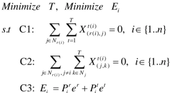
. In conclusion, the schedule goal of this paper has two points, i.e. (1) Minimize the time slot for convergecast. (2) Minimize the schedule energy consumption. The optimization problem is stated as below:

( )

( )

( ) ( ( ), ) 1

( ) ( , ) ,

,

. C1:

0,

{1.. }

C2:

0,

{1.. }

C3:

r i

r i j

i

T t i

r i j

j N t

T t i

j k

j N j i k N

r r t t

i i i

Minimize T

Minimize E

s t

X

i

n

X

i

n

E

P e

P e

∈ = ∈ ≠ ∈

=

∈

=

∈

=

+

∑ ∑

∑ ∑

(4)

The first condition ensures node receiving data at this slot will not send data. The second condition ensures the node receiving data will not be interferenced by other nodes. The third condition gives the calculation for nodal energy consumption.

IV. TDMA SCHEDULE ALGORITHM

a f e d c b s

Base Station g

h i

r

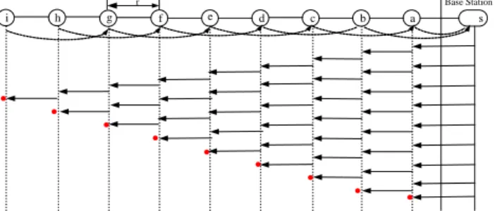
Fig. 1 TDMA scheduling in linear network whose hops k=1

In this way, for a given linear network’s schedule scheme, the time of last busy time slot (LBTS) of sink node just is the number of time slots required by the convergecast. In the 1-hop network in Fig. 1, the number of time slot that a whole network convergecast needs is

T=24.

Now, there is plenty of work for 1-hop networks, which can be found in Ref. [6, 9, 11]. However 1-hop network is the simplest network scene and its network performance and practicality are also restricted. We extend it in two aspects: Firstly, the TDMA scheduling scheme is extended for 1-hop networks to the general

k

-hop networks and the theoretical result is obtained for choosing the optimal value

k which makes the lifetime of general k -hop network longest. Secondly, the minimum TDMA scheduling time slot algorithm and the calculation formula in general

k-hop networks are presented. In the following paper, the schedule scheme of general k -hop network is given firstly, and then energy consumption is discussed. Finally, we analyze the TDMA scheduling time slot.

A. The Scheduling Algorithm

The idea of the TDMA schedule algorithm for general

k

-hop networks is as follows: For a k -hop network, the sink node sends data to the farthest node firstly, and then sends data to the second remote one, until the last node. For each node which has received data, as long as the nodes that is farther than it need to transmit data, then in the circumstances of the channel available, relaying the data forward with the maximum distance of no more than

k.

d

at the earliest possible time and sending it to destination nodes until all nodes in the network have received a datum.

However, the amount of data node k relays is the largest in above schedule approach. Especially when

n/3< k < n /2, the data of node k relays is about 1/3 to 1/2 of the entire network’s data, which makes the energy consumption of node k too large and results in the premature deaths of the network. Therefore, an improvement algorithm is proposed to balance the energy consumption of each node in this paper. The main purpose is to enable the amount of data network nodes relayed as balance as possible, which can extend the lifetime of the

network. The basic idea of it is similar to algorithm 1 in Ref. [8]. In algorithm 1 of Ref. [8], when nodes whose number are > = 3 k need to send data to the Sink, the node from 1 to k take turns to undertake the data transmission, and it sends k data in every 2 k +1 time slots. Consider those nodes with number large than 3k, when their data is sent, nodes numbering in

[ , 3 ]

k k

send their data firstly to

k

and then transmit to the destination. Hence, with Algorithm 1 in Ref[8], node with number k processes more data. In order to overcome the shortcomings of the above research, a load balancing schedule algorithm is proposed in this paper. The main idea is: As long as the >

k

nodes have data to send, then adopt the way in which the node from 1 to k take turns to undertake data transmitting, and the < k nodes send data directly. Based on the above analysis, Algorithm 1 presents the time slot scheduling procedure of the Sink node and nodes numbering 1 to k. For other nodes, when data is received, it would be sent to as far as possible if the channel is available.

In Algorithm 1, two major data structures are used: the first is pcline[1..n], which is used to save the received data amount. Obviously, when the elements in pcline[1..n] are all equal to one, every node receives one data packet that is sent to the Sink. The second data structure is the two dimensional array actionline[1..n,0..Maxstep], which is used to save nodal status in every time slot. actionline[i, step] represents the status of node i in time slot step. The node is sending data when this value is equal to 1. Otherwise, the node would be idling or receiving data when this value is equal to 0 and -1, respectively. Denote the last busy time slot (LBTS) of node j by T_j , i.e., actionline[i,step] is not equal to zero and the largest time slot is Tj. Obviously, the required time slots to complete a

linear network convergecast is: )

(

1i n Ti

Max

≤

≤ =Max(step)(|actionline[i, step]

≠

0).

Algorithm 1: A TDMA scheduling algorithm for balanced data routing in k -hop linear network

Algorithm1: TDMA time slot scheduling algorithm for k-hop network balance data routing

Input: WSG={v，l，p}，the value of the hops is k

Output: Two-dimensional array actionline[i, step] represents the status of the i-th node in the step-th time slot: T,R,I: sending, receiving, idleness

1) hop=k //hop means using how many hops to transmit data 2) m = MaxNode //m is the largest number of nodes in the network 3) Step=0 //step is the number of TS currently 4) Do While (step <= MaxStep)

Do While (i <= m)

actionline(i, step) = 0 i = i + 1

End do step = step + 1 End do

7) Do While (packets_left_K >=k)

//As long as the number of data which need to be transmitted //by the nodes whose id are greater than k For(i=k; i>=1; i--)

actionline[i, step]=R

//sink node send one data in each two time slot to //those nodes whose id are between 1 and k step=step+1

actionline[i, step]=T

//When those nodes whose id are from 1 to k receive //data, they send it forward in the next time slot step=step+1

End for step=step+1

packets_left_K= packets_left_K-k

// In the (2k+1)-th time slot, k data has been sent End do

8) i=k

9) Do While (packets_left_K >0)

//At this time, the number of data which need to be //transimitted by those nodes whose id are greater than k // is less than k.

actionline[i, step]=R //sink node sends a datum to node i step=step+1

actionline[i, step]=T

// When hose nodes whose id are from 1 to k receive data, //they send it forward in the next time slot

step=step+1 i=i-1

packets_left_K= packets_left_K-1 // send one data once End Do

10) Do While (packets_left >0)

//The id of the nodes which need to transmit data are less //than k at this time, and the remaining number of data is //packets_left.

actionline[i, step]=R

//sink send one data to node i (i is between 1 and k). //If all nodes in the current time slot can not send //data, then there is no operation.

step=step+1

packets_left= packets_left -1 //send one data once End Do

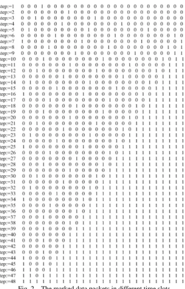
An example of Algorithm 1 is given in Fig.2. The number of nodes (including the Sink) is 26 and k =4. The Sink is on the left and not shown in the figure. There is no data at the beginning (marked by zero). At the beginning, the Sink has 25 data packets to transmit, and when each node received these packets, they are marked by one and the scheduling procedure is completed. Because every node has room for only one packet, it cannot receive more packets after it is marked by one. A node would continue to transmit the packet in some later time slot unless it is the destination. After retransmission, it’ll be remarked by zero to receive new packets. In Fig.3, the Sink would send its data packet to the farthest node (node 4) in the first time slot. During the second time slot, node 4 would transmit this packet to node 8 and other nodes would stop operating due to the interference. Node 4 would be marked by 0 and node 8 would be marked by 1 after the second time slot. This procedure would continue as shown in Fig.2.

Fig. 2 The marked data packets in different time slots Theorem 1: In the proposed TDMA scheduling algorithm1 for the k -hop linear network, the required storage capacity for each node to transmit data packets is not bigger than 1. Proof: In algorithm 1, each node can only be in three kinds of status, 1 as sending, 0 as idle, -1 as receiving. Due to status 0 has no affect on data storage capacity. Therefore, it only needs to consider the status of sending and receiving. In algorithm 1, the sending and receiving status of each node must be alternating, that is, when it is relaying data, it must receive data at first and when the node is in receiving state, the next operation is no operation or sending operation. The situation of receiving status will not appear twice continuously. It shows that each node can convergecast only with an additional storage capacity at any time.

■ Theorem 2: The amount of data the node ni whose id is

i in algorithm 1 needed to be sent is expressed as follows. In Eq. (5), Fix() is an integer function, that is, to take the integer part of the parameters.

t i

one data packet is relayed by node i . Hence the received number of data packets by node i is Fix((n−i)/k) and the sent data amount is equal to the relayed data amount plus its own data amount. Therefore, the data amount sent by node i is given by Eq. (5).

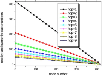
■ Thus, in the situation that each node generates the same data as the algorithm 1 in Ref. [8], the amount of data each node sent is relatively balanced than that in [8]. Fig. 3 shows that, although the data amount is large for nodes close to the Sink, the data amount is varying smoothly when k is increasing. This means the proposed algorithm could balance the network loads.

0 100 200 300 400 0 100 200 300 400 rec ei

ve and t

rans m int dat a num ber s node number hop=1 hop=2 hop=3 hop=4 hop=5 hop=6 hop=7 hop=8 hop=9

Fig. 3 The load every node undertakes

B. Analysis of energy consumption

The main analysis in this section is the energy consumption of node in different k hops, as well as how to obtain the optimal value of k so as to maximize the network lifetime. In practice, the actual size of the network

n

is very large when compared with k , that is,

n

>> k . Therefore in the following we only discuss the situation of

n

>>k.

0 10 20 30 40 50 60 70 0 1000 2000 3000 4000 5000 6000 7000 E ner gy c ons um pt ion( NJ ) node id hop=1 hop=2 hop=3 hop=4 hop=5 hop=6 hop=7 hop=8 hop=9 hop=10 hop=11

Fig. 4 The energy consumption of each node in Algorithm 1 Fig. 4 gives out the energy consumption of algorithm 1 under different k hop. k hop means the largest transmission distance is k⋅d, while the distance among nodes is

d

. In algorithm 1, the data of the nodes whose id

is from 1 to k is equally shared, and the sending distance of nodes which numbers are small is shorter, therefore the energy consumption is shorter than node k , because node

k undertakes the maximum amount of data, and its sending distance is the farthest, so its energy consumption is the largest. Fig. 4 reveals this scenario.

For a typical network [6, 8, 9, 11, 22], it can be seen from Fig. 4 that the maximum energy consumption node is node k (As those nodes whose id are between 1 and k undertake the same amount of data with the less sending distance of k , so the energy consumption is less the largest). In order to calculate convenient, we can use only node k to calculate the largest energy consumption node in algorithm 1 in the following.

Theorem 3: In algorithm 1, when the hop k meets

k= fs elec e E d 2 1

or

k

= d 1 4 3 2 amp elec E

ε , the network lifetime is

the largest.

Proof: Network lifetime can be defined as the time of energy depletion of the first node. Therefore to prolong the network lifetime is to prolong the lifetime of the node that firstly dead as possible as it can. That is to say that, the hop

k which makes the node that the consumption of the network is the largest consume the minimum energy is the optimal hop to let the network lifetime the longest. And the largest energy consumption node is node k . And its energy consumption can be seen from the following formula, in which

n k

is to take the integer part.

k

E =(2

n k

-1)Eelec+

n k

efs (

k

×

d

) 2

or

k

E =(2

n k

-1)E_elec+

n k

εamp (

k

×

d

) 4

While the formula above is the smallest, the network lifetime is the largest. It can be translated as follows:

k

E =2

n k

Eelec-Eelec+ nk efs 2 d or

k

E =2

n k

Eelec-Eelec+ 3

nk εamp 4

d

To make the formula above largest, derive it and make it 0: 2 2

1

2

fs elec

ne d

nE

k

−

=0 or

3

nk

2 _amp

d

4

2

nE

_elec

1

₂

k

ε

−

=0

Thus there is 2 ₂

. 2 d e E k fs elec

= or 4 ₄

. 3 2 d E k amp elec ε =

That is：k=

fs elec e E d 2 1

or k =

d

1

4 3 2 amp elec E ε ■

n

. As it can be seen in Fig. 5, when the number of node in network are 220, 320, 420 nodes respectively, the optimal value of

k

is the same. It means that the optimal value of

k

has nothing to do with the size of the network. While in Fig. 6, the optimal value of k increases with the reduction of d , which proves the conclusions of Theorem 3 to be correct.

5 10 15 20

0 2000000 4000000 6000000 8000000 10000000 12000000 14000000 16000000 18000000 20000000 E ner gy c ons um pt ion( NJ ) K n=220 n=320 n=420

Fig. 5 Energy consumption of the largest energy consumption nodes with different node in algorithm 1

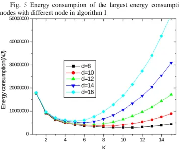
2 4 6 8 10 12 14 0 10000000 20000000 30000000 40000000 50000000 E ner gy c ons um pt ion( NJ ) K d=8 d=10 d=12 d=14 d=16

Fig. 6 Energy consumption of the largest energy consumption nodes with different d in algorithm 1

Corollary 1: In the proposed algorithm, the optimal hop

k

is not related to the network size, but related to the energy consumption parameters.

Proof: Theorem 3 has proved that when

k

=

1

(

2

E

_elec

)

e

_fs

d

or k = d

1 4 3 2 amp elec E

ε , the network

lifetime is the largest. The

k

at this time only has something to do with the parameter of the energy consumption but has nothing to do with the network size.

■ Theorem 4: Considering that the number of network nodes

a

k

s

n

=

×

+

|s>0, then in a convergecast cycle, the residue energy El_eft in algorithm 1 can be expressed as

follows:

eft l

E

=

E

_left1..(k−1)+

E

_left(k+1)..n

1

1..( 1) 1 ( 1).. 2 2

1 1

, ( 1) ( 1) / 2

k a

k k n

left i j left elec fs i j

E s E E E k s sE s ε k d

−

− +

= =

=

∑ ∑

− = − + −

2 2 2 2 1 2 2

, 2

i fs fs j elec fs

E

= −

ε

k d

ε

i d

= +

E

E

ε

j d

(6)

Proof: Assuming that the total number of network nodes

is

n

, it can be expressed as

n

=

s

×

k

+

a

} / ... 2 , 1 {

|s∈ n k ,a∈{0,1,..k−1} for the fact that the energy of node k depleted at first. Hence, after each convergecast, we compute the energy decrease consumed by other nodes compared with node k , which is the residual energy after one convergecast.

The calculation is divided into three parts. Energy that less than node k uses: (1)

i

∈

{1..

a

}，(2)

i

∈

{

a

+1..

k

-1}，(3)

i

∈

{

k

+1..

n

}.

(1) Firstly, compute the residual energy from node 1 to node

a

. These nodes receive and transmit one more packet than node

k

in one convergecast cycle and they consumption more energy. But the distance of sending data of these nodes is smaller than that of node

k

(which consumes the highest energy), therefore their remained energy compared to node

k

is computed by:

2 2

d k E

Ej = elec+εfs

-2 2

d j

Eelec−εfs | j∈{1...a}

In addition, the energy consumed for sending and transmitting one more data is E1j=2Eelec+εfsj2d2

s data packets are required to be sent in one convergecast cycle, therefore, the residual energy is given by:

∑

₌ ⋅ a j j E s 1 -

∑

= a j j E 1 1 (7)

(2) The amount of data sent and received by those nodes whose id are between

i

(

i

=

a

+1) and

k

-1 is the same as that of node

k

, but as energy consumed for receiving data is the same as that of node k . The residual energy is because the distance for data transmission is less than that of node k . Therefore, the decreased energy of sending one packet is given by:

i

E =εfsk2d2 -2 2

d i

fs

ε |i∈{a+1...k−1} (8)

s

data packets are required to be sent in one convergecast cycle. Therefore, the residual energy is

∑

−₊ = ⋅ 1 1 k a i i E

s . Combine Eq. (7) with Eq. (8), the following

equation can be obtained:

1 1

1..( 1) 1 1

1 1 1 1 1

k a a k a

k

left i j j i j

i a j j i j

E s E s E E s E E

− −

− =

+=

∑

= +

∑ ∑

= − = =

∑ ∑

= −

(9)

(3) The residual energy of { k +1…n} node

The energy consumption from node k to node

k

+

a

For those nodes whose id are between

k

+

a

+1 and 2

k

+

a

, these nodes receive and transmit one less packet than node k , but the transmission distance is the same, i.e.,

kd. Therefore the residual energy is the energy to send and receive one data packet:

) 2

( 2 2

1 k E k d

Ek = elec+εfs (10)

Similarly, those nodes whose id are between 2 k +

a

+1 and 3 k +

a

process two less data packets than node k , and so their residual energy is equal to the energy for transmitting and receiving two packets:

) 2

4

( 2 2

2 k E k d

E k= elec+ εfs (11)

With similar logic, those nodes whose id are between (

s

-1)

k

+

a

+1 and

sk

+

a

process

s

-1 less data packets than node k , and so their residual energy is equal to the energy for transmitting and receiving

s

-1 packets:

) )

1 ( ) 1 ( 2

( 2 2

1 k s E s k d

Es− = − elec+ − εfs (12)

Therefore the residue energy of those nodes whose id are from

k

+1 to

n

in a convergecast cycle is

E

_left(k+1)..n

(

)

(

)

(

)

1

( 1).. 2 2

1

2 1 2,...

1

1 2,...

1

s

k n

left ik elec fs

i

E

E

k

s

E

s

ε

k d

− +

=

=

∑

=

+ + −

+ + + −

=

k

(

( )

s 1 s

−

E

elec

+ −

( )

s 1 s

ε

fs

k d

2 2

2

)

(13)

Combination of Eq. (9) and Eq. (13), the total energy residue in a convergecast cycle is

eft l

E

=

E

_left1−(k−1)+

E

_left(k+1)−n

■ The proportion of energy residue in network refers to the proportion of the total energy to the initial total energy when the first node dead. It can be defined as follows:

left

µ

=

k left

E

n

E

.

if s>0

k

E

sE

elec

s

fs

k

d

(

s

1

)

E

elec

2

2

+

−

+

=

ε

else

0 50 100 150 200 250 300 350 400 450 0.4

0.5 0.6 0.7 0.8

lef

t ener

gy

r

at

io

K d=8

d=10 d=12 d=20

Fig. 7 The energy utilization under different d in algorithm 1 Fig. 7 and Fig. 8 show the energy utilization under different network parameters. The curves are zigzagged.

Based on Theorem 2, each node process Fix((n−i)/k)+1 data packets, and thus the most energy consuming nodes process the same data packets when k is within some range. But when the distance increases and the energy consumption also increases, the number of relayed data packet is reduced by one when (n−i)modk=0. Hence the consumed energy is suddenly reduced and increased, which is shown as zigzagged curves.

0 50 100 150 200 250 300 350 400 450 0.4

0.5 0.6 0.7 0.8

d=10

lef

t ener

gy

r

at

io

k

n=300 n=350 n=400 n=450

Fig. 8 The energy utilization under different network size in algorithm 1

Theorem 5: With the proposed algorithm, for a large-scale network with the number of nodes is

n

, and adopt parameters that make the network lifetime the longest, if

n

>>

k

, when the network dies, the residue energy in algorithm 1 is nearly 50%.

Proof: Suppose the number of nodes in the network is

a

k

s

n

=

×

+

. When

n

>> k (s can be considered approximately equal to

n

) and the parameter leading to the longest network life is used, the energy utilization of

the proposed algorithm 1 is

µ

_left=

k left

E n E

. . From Theorem 4

we know

E

_left is the residual energy for nodes 1…

k

and

nodes i (i>

k

). Because

k

is much smaller than n, and the residual energy for these nodes is small, their residual energy could be neglected during calculation and so

left

E

≈

n

(

s

-1)

E

_elec +

n

(

s

-1)

ε

_fs

k

2

d

2 /2 and

k

nE

=

n

(

sE

_elec

+

s

ε

_fs

k

2

d

2

+

(

s

−

1

)

E

_elec

)

. We hence

know

µ

_left

≈

50% if

n

is large.

■ Fig. 9 illustrate this situation that when

k

gets the optimal value; the residue energy in algorithm 1 is nearly 50%.

Lemma 1: When the residual energy of network is the lowest, it does not mean that the network lifetime is the longest.

the network life

k

is not the longest. In algorithm 1,

k

has a small value. So, in Fig. 8, when

k

=155, the residual energy is the lowest. Obviously, the longest network life is not in accordance with the lowest residual energy.

■

2 4 6 8 10

0.40 0.42 0.44 0.46 0.48 0.50 0.52 0.54 0.56 0.58 0.60

lef

t ener

gy

r

at

io

K n=300 n=350 n=400 n=450

Fig. 9 when n>>k, the ratio of the residue energy is approximately 50%

0 5 10 15 20 25 30 35 40

60 80 100 120 140 160 180

T

S

Hops Node=20 Node=25 Node=30 Node=35

Fig. 10 The number of time slots required for scheduling under networks of different sizes and different k in algorithm 1

Network lifetime is an important performance index for sensor network. Lemma 1 illustrates that in sensor network, the one that energy utilization is the maximum (referring to the smallest residue energy) is not always the optimal network. This means that the optimization of sensor networks energy needs to be improved from the following two aspects simultaneously to improve network lifetime: 1) Reduce the energy consumption of the maximum energy consumption node; 2) Reduce the energy consumption rate of sending a unit data in network. In addition, Theorem 5 illustrates in general network, when the network dies, the residue energy is relatively large. For example, when the nodes that near the sink are communal nodes of several linear networks, they need to undertake several linear branches of data at the same time, then the network lifetime will be a fraction of the original, for the nodes which undertake more than six branches, when the network dies,

the residue energy rate will be at least as high as 90%. While it is common. So it can be seen that the conclusions of this paper is of universal significance.

C. The TDMA time slot scheduling

Theorem 6: When the size of the network is

n

, and the hops are

k

, the number of TDMA cycle time slots in algorithm 1 needs is:

3

1

2

−

+

=

n

k

k

TS

=3

n

-3

if

k

=

1

≤

TS

k

k 1

2

+

)

(

n

−

k

+

k

if

k

=

1

Proof: 1) When

k

=1, at most after

n

-3 TS delay, the first data packet would be sent to node C, which is a 3-hop node. After that, node C could transmit one data packet in every

k

k 1

2

+

=3 TS (3 TS is needed to complete 1 cycle due to

channel interference, i.e., data sending status, idling status,

data receiving status). After 3

∑

≥ n

j 3

1

TS, 当

k

=1时，the

last data packet of node

j

(>=3) must have been sent to node C that requires 2 TS to transmit all the data packets

from node

j

to the Sink. The spent time is

k

k 1

2

+

(

n

-2).

One data packets from node 1 and 2 are needed for transmission. Node 1 and 2 requires 1 TS and 2 TS for one packet and so totally 3 TS is needed. The number of overall

time slots is not bigger than

k

k 1

2

+

(

n

-2)+3=3

n

-3 TS.

2) When

k

>1, the nodes whose hops are larger than

k

send

k

data packets in every 2

k

+1 cycles, similar to the case in Fig.7. The nodes whose hops are less than or equal to

k

send one data packet in every TS. Q.E.D.

■ Fig. 10 represents the number of time slots required in algorithm 1 for an entire network convergecast with different hops k. The results and the analysis result of Theorem 6 is consistent.

V. CONCLUSION

scheduling time slot and network lifetime. In addition, extensive simulation experiments have been conducted and results are consistent with the theoretical results.

REFERENCES

[1] A. F. Liu, X. Jin, G. H. Cui,Z. G. Chen. "Deployment Guidelines for Achieving Maximal Lifetime and Avoiding Energy Holes in Sensor Network," Information Sciences, vol. 230, pp. 197–226, 2013. [2] L. S. Jiang, A. F. Liu, Y. L. Hu, Z. G. Chen. "Lifetime Maximization

through Dynamic Ring-Based Routing Scheme for Correlated Data Collecting in WSNs," Computers & Electrical Engineering,vol.41, no. 1, pp. 191–215, 2015.

[3] L. W. Yeh, M. S. Pan. "Beacon scheduling for broadcast and convergecast in ZigBee wireless sensor networks," Computer Communications, vol. 38, pp. 38: 1-12, 2014.

[4] T. S. Chen, H. W. Tsai, Y. H. Chang, et al. "Geographic convergecast using mobile sink in wireless sensor networks," Computer communications, vol. 36, no. 4, pp. 445-458, 2013.

[5] S. He, X. Li, J. Chen, et al. "EMD: Energy-Efficient Delay-Tolerant P2P Message Dissemination in Wireless Sensor and Actor Networks," IEEE Journal on selected area in communications, Vol.31, no. 9, pp. 75-84, 2013.

[6] C. Florens, R. McEliece. "Packets distribution algorithms for sensor networks," IEEE INFOCOM 2003. Twenty-Second Annual Joint Conference of the IEEE Computer and Communications. Vol. 2, pp. 1063-1072, 2003.

[7] C. Kam, C. Schurgers. "ConverSS: A Hybrid MAC/Routing Solution for Small-Scale, Convergecast Wireless Networks," IEEE Transactions on mobile computing, vol. 10, no. 9, pp. 1227-1236, 2011.

[8] A. Liu, J. Xu, Z. Chen. "A TDMA scheduling algorithm to balance energy consumption in WSNs," Computer Research and Development, vol. 47, no. 2, pp. 245-254, 2010.

[9] S. Gandham, Y. Zhang, Q. Huang. "Distributed minimal time convergecast scheduling in wireless sensor networks," 26th IEEE International Conference on Distributed Computing Systems, pp. 50-50, 2006.

[10] A. Liu, D. Zhang, P. Zhang, et al. "On mitigating hotspots to maximize network lifetime in multi-hop wireless sensor network with guaranteed transport delay and reliability," Peer-to-Peer networking and applications, vol. 7, no. 3, pp. 255-273, 2014.

[11] A. Hossain, T. Radhika, S. Chakrabarti, et al. "An Approach to Increase the Lifetime of a Linear Array of Wireless Sensor Nodes," International Journal of wireless information networks, vol. 15, no. 5, pp. 72-81,2008. [12] A. Liu, J. Ren, X. Li X, et al. "Design principles and improvement of

cost function based energy aware routing algorithms for wireless sensor networks," Computer networks, vol. 56, no. 7, pp. 1951-1967, 2012. [13] Y. X. Liu, A. F. Liu, Z. G. Chen. "Analysis and Improvement of

Send-and-Wait Automatic Repeat-reQuest protocols for Wireless Sensor Networks," Wireless personal communications, vol. 81, no. 3, pp. 923-959, 2015.

[14] M. Dong, K. Ota, M. Lin, et al. "UAV-assisted data gathering in wireless sensor networks," The Journal of Supercomputing, vol. 70, no. 3, pp. 1142-1155, 2014.

[15] Q. Chen, S. S. Kanhere, M. Hassan. "Analysis of per-node traffic load in multi-hop wireless sensor networks," IEEE transactions on wireless communications, vol. 8, no. 2, pp. 958-967, 2009.

[16] J. Wu, B. Cheng, C. Yuen, Y. Shang, J. Chen. "Distortion-Aware Concurrent Multipath Transfer for Mobile Video Streaming in Heterogeneous Wireless Networks," IEEE transactions on mobile computing. DOI: 10.1109/TMC.2014.2334592.

[17] Y. Hu, M. Dong, K. Ota, et al. "Mobile Target Detection in Wireless Sensor Networks With Adjustable Sensing Frequency," IEEE system Journal. http://dx.doi.org/10.1109/JSYST.2014.2308391.

[18] X. Xu, X. Li, X. Mao, et al. "A delay-efficient algorithm for data aggregation in multihop wireless sensor networks," IEEE transactions on parallel and distributed systems, vol. 23, no. 1, pp. 163-175, 2011. [19] C. Y. Ngo, V. O. K Li. "Centralized broadcast scheduling in packet radio

networks via genetic-fix algorithms," IEEE transactions on communications, vol. 51, no. 9, pp. 1439–1441, 2003.

[20] W. Shang, P. Wan, X. Hu. "Approximation algorithm for minimal convergecast time problem in wireless sensor networks," Wireless networks, vol. 16, no. 5, pp. 1345-1353, 2010.

[21] S. Huang, P. Wan, C. Vu, et al. "Nearly constant approximation for data aggregation scheduling in wireless sensor networks," Proceedings of the 26th Conference on Computer Communications. INFOCOM 2007, pp. 366–372, 2007.

[22] A. Liu, X. Wu, Z. Chen, W. Gui. "An Energy-balanced Data Gathering Algorithm for Linear Wireless Sensor Networks," International Journal of wireless information networks, vol. 17, no. 1-2, pp. 42-53, 2010. [23] A. Liu, P. Zhang, Z. Chen. "Theoretical analysis of the lifetime and

energy hole in cluster based Wireless Sensor Networks," Journal of parallel and distributed computing, vol. 71, no. 10, pp. 1327-1355, 2011. [24] H. M. Ammari, S. K. Das. "trade-off between energy and delay in data

dissemination for wireless sensor networks using transmission range slicing," Computer communications, vol. 31, pp. 1687–1704, 2008. [25] J. Long J, M. Dong, K. Ota, et al. "Achieving source location privacy

and network lifetime maximization through tree-based diversionary Routing in wireless sensor networks," IEEE access, vol. 2, pp. 633-651, 2014.

[26] S. He, J. Chen, F. Jiang, et al. "Energy Provisioning in Wireless Rechargeable Sensor Networks," IEEE transactions on mobile computing, Vol.12, no. 10, pp.1931-1942, 2013.

[27] J. Wu, C. Yuen, B. Cheng, Y. Shang, J. Chen. "Goodput-aware load distribution for real-time traffic over multipath networks," IEEE transactions on parallel and distributed systems. DOI: 10.1109/TPDS.2014.2347031.

[28] M. Dong, K. Ota, X. Li, et al. "HARVEST: a task-objective efficient data collection scheme in wireless sensor and actor networks," The Third International Conference on Communications and Mobile Computing (CMC), pp. 485-488, 2011.

Jun Long is a Professor of School of Information Science and Engineering of Central South University, China. His major research interest is wireless sensor network.

Mianxiong Dong received B.S., M.S. and Ph.D. in Computer Science and Engineering from the University of Aizu, Japan. He is currently an Assistant Professor with Muroran Institute of Technology, Japan. His research interests include wireless sensor networks, vehicular ad-hoc networks, and wireless security.

Kaoru Ota received MSc degree at Oklahoma State University, US in 2008 and Ph.D degree at the University of Aizu, Japan in 2012. She is an Assistant Professor with Muroran Institute of Technology, Japan. Her research interests include wireless networks and ubiquitous computing.