Article
New Algorithm for Evaluating the Green Supply
Chain Performance in an Uncertain Environment
Pan Liu and Shuping Yi *
College of Mechanical Engineering, Chongqing University, Shazheng Road 174, Chongqing 400044, China; [email protected]
* Correspondence: [email protected]; Tel.: +86-23-6510-6939 Academic Editor: Marc A. Rosen
Received: 29 April 2016; Accepted: 12 September 2016; Published: 26 September 2016
Abstract: An effective green supply chain (GSC) can help an enterprise obtain more benefits and reduce costs. Therefore, developing an effective evaluation method for GSC performance evaluation is becoming increasingly important. In this study, the advantages and disadvantages of the current performance evaluations and algorithms for GSC performance evaluations were discussed and evaluated. Based on these findings, an improved five-dimensional balanced scorecard was proposed in which the green performance indicators were revised to facilitate their measurement. A model based on Rough Set theory, the Genetic Algorithm, and the Levenberg Marquardt Back Propagation (LMBP) neural network algorithm was proposed. Next, using Matlab, the Rosetta tool, and the practical data of company F, a case study was conducted. The results indicate that the proposed model has a high convergence speed and an accurate prediction ability. The credibility and effectiveness of the proposed model was validated. In comparison with the normal Back Propagation neural network algorithm and the LMBP neural network algorithm, the proposed model has greater credibility and effectiveness. In practice, this method provides a more suitable indicator system and algorithm for enterprises to be able to implement GSC performance evaluations in an uncertain environment. Academically, the proposed method addresses the lack of a theoretical basis for GSC performance evaluation, thus representing a new development in GSC performance evaluation theory.
Keywords: green supply chain; performance evaluation; Rough Set; Genetic Algorithm; Levenberg Marquardt Back Propagation
1. Introduction
In recent years, concerns regarding environmental problems have increased. To react to this trend, many investigators [1–3] have begun to explore the aspects of a green supply chain (GSC) in which GSC performance evaluation is a vital issue. Because an inefficient GSC will lead to wasted resources and extra costs, the GSC performance evaluation problem is an urgent issue to be addressed by companies.
The purpose of this study was to contribute solutions to the GSC performance evaluation problem. Although many performance indicators [4,5] and methods [6–10] for GSC performance evaluation have been proposed, the bionics method was considered to be the effective one that could be used in different areas. Consequently, many optimization algorithms based on bionics have been proposed, including the Levenberg Marquardt Back Propagation neural network algorithm (LMBP neural network algorithm) [10], the Fuzzy Neural Network [11], the Bees Algorithm [12], the Ant Colony Optimization [13], and a Genetic Algorithm (GA) [14]. Among these algorithms, neural network algorithms have been widely used to evaluate supply chain performance. Among these neural network algorithms, the LMBP neural network algorithm has been demonstrated to be an effective method for evaluating supply chain performance [10]. However, this method easily falls into a local minimum
point. GA is a widely used method that has a good overall optimization nature. Therefore, a method that combined GA with the LMBP neural network algorithm (GA-LMBP neural network algorithm) was proposed and used in many areas [15–18]. However, this method has rarely been applied for supply chain performance evaluation. The problem regarding the evaluation of supply chain performance has also faced fuzzy uncertainty. In the decision-making process, a rough and uncertain environment has also often been encountered. Rough Set theory (RS theory) is thought to be an effective method to address the uncertainty of the evaluation environment. Therefore, a method combining the GA-LMBP neural network algorithm with RS theory (RS-GA-LMBP neural network algorithm) will have great potential for GSC performance evaluation. Studying this method is important and necessary.
Among the current indicator systems, the five-dimensional balanced scorecard (5DBSC) was considered a more comprehensive indicator system and was classified as the most influential management theory; however, it could not evaluate green performance very well. Although many studies were able to address this gap, some limitations remained: (a) some indicators contained in the 5DBSC were not clearly measurable; and (b) the measurement methods of some indicators were not consistent with the IOS 14000 Environment Management Standard. Therefore, it was important to revise the 5DBSC to address the above limitations.
To address the deficiencies of prior studies, a new method of combining the GA-LMBP neural network algorithm with RS theory was proposed based on an improved 5DBSC. According to the previously noted studies and the ISO 14000 Environment Management Standard, an improved 5DBSC was first proposed. Then, an RS-GA-LMBP neural network algorithm was presented. Finally, a case study was implemented to test its validity and reliability.
A new method for GSC performance evaluation was proposed, constituting a new development in the theoretical basis of GSC performance evaluation. The method can not only accurately evaluate the level of GSC performance but also provide solutions to optimize and improve GSC performance. In practice, the proposed method was implemented based on a case study. By optimizing the performance of supply chain core enterprise, the proposition that performance evaluation methods could guide business practices was achieved. In this way, the operational efficiency and effectiveness of the supply chain can be fully enhanced.
This article is organized as follows: Section1presents the introduction; Section2presents the indicator systems and methods for GSC performance evaluation; Section3presents the algorithms for GSC performance evaluation; Section4presents the improved 5DBSC; Section 5presents the related algorithms of the RS-GA-LMBP neural network algorithm; Section6presents the model of the RS-GA-LMBP neural network algorithm; Section7presents the case study; and Section8presents the study’s conclusions.
2. Indicator Systems and Methods of GSC Performance Evaluation
GSC management has been described as the combination of green purchasing and supply chain management from a supplier to customers, manufacturers, and reverse logistics [19]. Companies have often expected their suppliers to undertake environmental compliance and other related activities [20]. Therefore, the selection and evaluation of suppliers have been studied by many investigators [20,21]. However, the supplier evaluation could not react to the entire supply chain performance and cooperative situations among companies, causing the GSC to lose competitive advantages.
To improve and effectively manage GSC performance, GSC management has been used and studied by many researchers [22–25]. GSC management practices could achieve a win-win situation of environmental performance and economic performance [19]. However, the economic outcomes were dependent on not only the implementation of the green plan but also the effectiveness of the GSC. Therefore, the performance evaluation of a GSC is increasingly vital.
three areas (resources, output, and flexibility) was proposed [27]. Next, a supply chain operation reference that was the first global evaluation model of the standard supply chain process was proposed by two firms in the USA [28]. In addition, Key Performance Indicators (KPI) [29] were developed and used in supply chain performance evaluation. This was a tool that divided the strategic goals of an enterprise into operational goals and was used in Product Lifecycle Management (PLM) [30]. To evaluate the revenues gained by adopting a PLM tool, a method was proposed based on KPI [31], and its effectiveness was tested by an Aerospace and Defense company [31]. In 1992, the balanced scorecard was proposed by Kaplan et al. [32]. In earlier studies, the indicators of this scorecard included four parts: (a) the accounting section; (b) a customer section; (c) an internal business process section; and (d) a learning and development section. The advantages of the balanced scorecard were that it adopted the successful experiences of other companies or other industries and used them as the evaluation standard to evaluate the supply chain of the company using the scorecard. This practice allowed the company using the scorecard to catch up with or exceed the supply chain performance attained by other companies.
Among the evaluation methods described above, the balanced scorecard was thought to be a more comprehensive, simple, and clearly defined objective indicator system. It was classified as the most influential management theory in recent years by the Harvard Business Review. In addition, according to an authoritative survey by Fortune magazine, more than 55 percent of the top 1000 companies have implemented the balanced scorecard [10]. The selection of balanced scorecard indicators has been closely linked with company strategy. Each type of indicator provides a specific measure of corporate performance.
The models of balanced scorecards are different. From the aspects of production flexibility, cash turnover time, order indicators, and material flow, the balanced scorecard has been used for supply chain performance evaluation [33]. However, the balanced scorecard has a defect that has been described as “cause and effect relationships and time delay, and its variables could be either causes or results and their relationships were not linear” [34]. In addition, the suppliers’ performance indicators were not contained in the balanced scorecard. Therefore, the 5DBSC, having five different aspects, has been proposed [35]. This research added supplier performance into the balanced scorecard indictor system and addressed the shortcomings of the indicator system of the original balanced scorecard.
However, the 5DBSC did not contain green performance indicators. Therefore, efforts to study green performance were conducted. Kurnia et al. [36] proposed a measurement method for the sustainability performance for industrial networks. Economic performance, environmental performance, and societal performance were contained in this method, similar to the research of Seuring et al. [37]. However, this method was not combined with the 5DBSC. Consequently, many investigators added green performance into the 5DBSC. Bhattacharya et al. [4] and Duarte et al. [38] improved the GSC performance indicators based on an integrated approach with the balanced scorecard. However, the measurement methods of performance indicators presented in the previously noted papers were not clear. In addition, Shao et al. [39] added the environmental indicators (i.e., energy usage rate and environmental pollution) to indicate the green level of a GSC. However, the environmental indicators could not completely describe green performance. Chen et al. [40] explored GSC performance evaluation indicators. In their indicator system, green performance indicators (i.e., energy saving rate, environmental pollution, green procurement rate, and green recovery rate) were included in the 5DBSC. However, the measurement method of “environmental pollution” did not correspond with the IOS 14000 Environment Management Standard.
Based on the previously noted investigations and the IOS 14000 Environment Management Standard, an improved 5DBSC was proposed. The primary contribution of the improved is that the concept of “environmental pollution” in Chen’s study [40] was improved. This pollution measurement is determined using the total emissions of “three wastes”. A detailed description is provided in Section4.
3. Nature-Inspired Algorithms and Their Applications to GSC Performance Evaluation
3.1. Nature-Inspired Algorithms
Many bionic algorithms have been proposed to evaluate supply chain performance. The Bees Algorithm [12] is an optimization technique that imitates the behavior of bees and has a particular application to intelligent cluster thinking. Its main feature is that special information of issues is not necessary. However, when the local optimal solution is sought, the convergence speed becomes slow. In addition, it is easy to fall into a local optimum. The Ant Colony Optimization [13] is a probability algorithm that is used to find the optimal path in a figure. Compared with other algorithms, the Ant Colony Optimization requires less initial route information; however, it takes a long time to reach the optimal solution and has a low convergence. GA is a stochastic search method based on imitating biological evolution [14]. In the areas of global optimization, planning and control engineering, GA has been widely used to address many complicated problems. Its advantage is that it can easily reach the global optimal solution. However, it is easy to advance the convergence speed. The artificial neural network algorithm is an algorithm that simulates human thinking. It is also used in many areas [41–43], such as decision making, data mining, and sequence recognition. Although the artificial neural network algorithm has some limitations in evaluating supply chain performance, many investigators have supported its use.
3.2. Applications of Nature-Inspired Algorithms to GSC Performance Evaluation
Among the above algorithms, the GA and artificial neural network algorithms have been widely used for evaluating supply chain performance evaluation.
(1) The application of GA
The GA has a good overall optimization nature and has been used in many areas. For example, Zhang et al. [44] used the GA to analyze supply chain performance. In addition, it was used to solve the transport issues of a railway network [45]. The optimization of GA does not depend on gradient information. Moreover, it can prevent the objective function from being trapped in a local optimal state [46].
(2) Applications of neural network
supply chain performance. However, the LMBP neural network algorithm had some limitations such as the fact that the optimal solution can easily fall into a local optimum.
To improve the search speed and avoid solutions falling into the local optimum, the advantageous elements of GA were used to optimize the initial weights and thresholds of the neural network. Therefore, a GA-LMBP neural network algorithm has been proposed. In fact, it has been used in many areas such as predicting water-assisted injection [15], analog circuit fault diagnosis [16], and harmful algal blooms prediction [17]. Moreover, the GA-LMBP neural network algorithm has also been used to evaluate passenger comfort with respect to vibration in railway vehicles [18]. These applications have demonstrated that the GA-LMBP neural network algorithm is more effective than the BP neural network algorithm. However, the applications of the GA-LMBP neural network algorithm to the evaluation of supply chain performance have been few.
The problem of evaluating the supply chain performance faces fuzzy uncertainty, sources uncertainty, and random uncertainty. In a decision-making process, a rough uncertain environment must often be addressed. RS theory has been considered an effective method for use in an uncertain evaluation environment. It was thought to be a suitable and effective method for dealing with qualitative data [50]. RS theory has also been used together with many other methods, such as data envelopment analysis [51] and the LMBP neural network algorithm [52]. These studies demonstrated that RS theory is an effective method to reduce the data of the unnecessary indicators. However, there are still few investigations combining the GA-LMBP neural network algorithm with RS theory.
To address these gaps, a new method called the RS-GA-LMBP neural network algorithm has been proposed. Here, RS theory is used to remove the redundant evaluation indicators and reduce the unnecessary data. GA is utilized for searching and optimizing the initial weights and threshold values of the neural network. The local fast convergence and the network parameters’ optimization uses the LMBP neural network algorithm.
The RS-GA-LMBP neural network algorithm uses the advantages of RS theory to remove unnecessary data. This network overcomes the shortcomings of the LMBP neural network algorithm (i.e., the fact that it is easy to fall into a local minimum point). In addition, the RS-GA-LMBP neural network algorithm can easily reach the global solution. It can also be used in many evaluation problems, but it was first used for GSC performance evaluation.
4. Improved 5DBSC
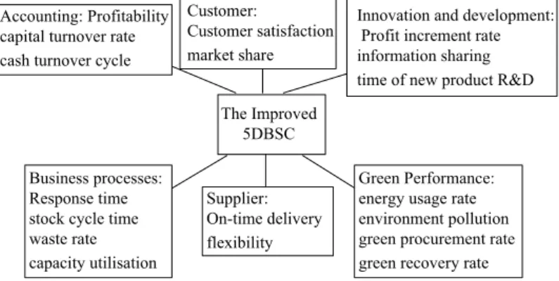
Based on the IOS 14000 Environment Management Standard and the study of Zhu et al. [19], the concept of “environmental pollution” in Chen’s study [40] was improved, and the extent of the “environmental pollution” was measured using the total emissions of “three wastes”. Therefore, the improved 5DBSC will be used to build the performance evaluation model of a GSC, as shown in Figure1and Table1.
The Improved 5DBSC Accounting: Profitability
capital turnover rate cash turnover cycle
Customer:
Customer satisfaction market share
Innovation and development: Profit increment rate information sharing time of new product R&D
Business processes: Response time stock cycle time waste rate capacity utilisation
Supplier: On-time delivery flexibility
Green Performance: energy usage rate environment pollution green procurement rate green recovery rate
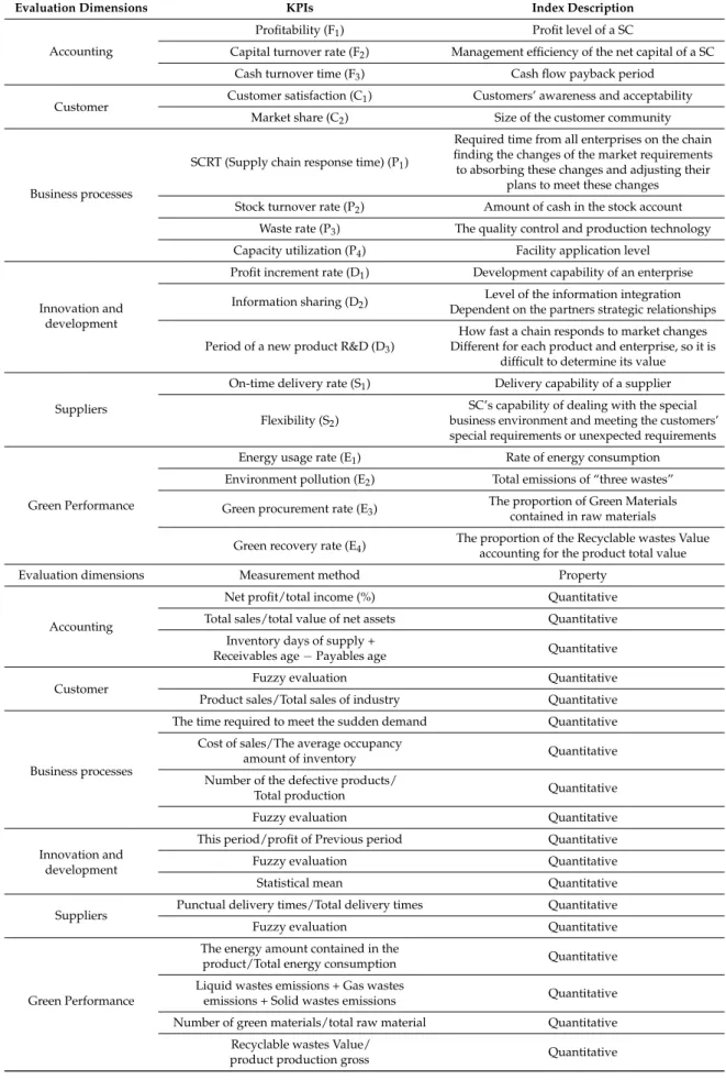
Table 1.The indicators of the improved 5DBSC.
Evaluation Dimensions KPIs Index Description
Accounting
Profitability (F1) Profit level of a SC
Capital turnover rate (F2) Management efficiency of the net capital of a SC
Cash turnover time (F3) Cash flow payback period
Customer Customer satisfaction (C1) Customers’ awareness and acceptability Market share (C2) Size of the customer community
Business processes
SCRT (Supply chain response time) (P1)
Required time from all enterprises on the chain finding the changes of the market requirements to absorbing these changes and adjusting their
plans to meet these changes Stock turnover rate (P2) Amount of cash in the stock account
Waste rate (P3) The quality control and production technology
Capacity utilization (P4) Facility application level
Innovation and development
Profit increment rate (D1) Development capability of an enterprise
Information sharing (D2) Dependent on the partners strategic relationshipsLevel of the information integration
Period of a new product R&D (D3)
How fast a chain responds to market changes Different for each product and enterprise, so it is
difficult to determine its value
Suppliers
On-time delivery rate (S1) Delivery capability of a supplier
Flexibility (S2)
SC’s capability of dealing with the special business environment and meeting the customers’ special requirements or unexpected requirements
Green Performance
Energy usage rate (E1) Rate of energy consumption
Environment pollution (E2) Total emissions of “three wastes”
Green procurement rate (E3) The proportion of Green Materialscontained in raw materials
Green recovery rate (E4) The proportion of the Recyclable wastes Valueaccounting for the product total value
Evaluation dimensions Measurement method Property
Accounting
Net profit/total income (%) Quantitative Total sales/total value of net assets Quantitative
Inventory days of supply +
Receivables age−Payables age Quantitative
Customer Fuzzy evaluation Quantitative
Product sales/Total sales of industry Quantitative
Business processes
The time required to meet the sudden demand Quantitative Cost of sales/The average occupancy
amount of inventory Quantitative Number of the defective products/
Total production Quantitative
Fuzzy evaluation Quantitative
Innovation and development
This period/profit of Previous period Quantitative
Fuzzy evaluation Quantitative
Statistical mean Quantitative
Suppliers Punctual delivery times/Total delivery times Quantitative
Fuzzy evaluation Quantitative
Green Performance
The energy amount contained in the
product/Total energy consumption Quantitative Liquid wastes emissions + Gas wastes
emissions + Solid wastes emissions Quantitative Number of green materials/total raw material Quantitative
Recyclable wastes Value/
5. Related Algorithms of the RS-GA-LMBP Neural Network Algorithm
5.1. RS Theory
RS theory was introduced to address defective and blurry concepts [50], such as data sets S= (U,A,V,f), where,U={x1,x2, . . . ,xn}is a set of limited and non-empty targets, Ais the set of attributes that could be used to characterize the targets, andVis the region of the attribute values. The information function is f, f :U×A→V.
With random attributes B ⊆ A, there is a correlated indiscernible connection I ND(B) : I ND(B) = {(x,y)∈U×U| ∀a∈B,f(x,a) = f(y,a)}. (x,y) ∈ I ND(B), which expresses that targetsxandyare invisible with respect toB, and[xi]B={x|(xi,x)∈ I ND(B),x∈U}.
In the information system, a random subsetXis given in which the following can be expressed:
(
BX={[x]B|[x]B∈X,x∈U}
BX={[x]B|[x]B∩X6=∅,x∈U}
BX and BX are called the lower and upper limits of X in terms of B, respectively. For an indescribable set, this value could be called a RS. BND(X) = BX−BX is the range of the approximate value.
Assume thatC is the group of the condition property set and Dis the decision inU. Then, two separations of the universeCandDwould form. ApproachingU/DwithU/C, the side ranges are calledPOSC(D) = ∪
X∈U/DCX,BNDC(D) =X∈U∪/DCX−X∈U∪/DCX.
For anyB⊆C, a decision table will be given. The decision property setDrelies onBwith a level kand is indicated byB⇒kD, where
k=γB(D) = |
POSB(D)|
|U|
A decision table DT = (U,C∪D,V,f), if P ⊆ Q ⊆ C, γQ(D) ≥ γP(D) is generated. If DT= (U,C∪D,V,f), B ⊆ C and a ⊆ B, then a is redundant. If γB(D) = γC(D) and
∀a∈ B:γB(D)>γB−a(D), thenBis a reduct of the table. If(U,C∪D,V,f)is a decision table and
Bj
j≤r is the set of reducts, then the following can
be expressed:
Core= ∩
j≤rBj−Core Kj=Bj−Core,I=A− ∪
j≤rBj.
Coreis the property subset. Iis called the totally irrelevant property set. Kjis a poor pertinent property set. The alliance ofCoreandKjproduce a reduct.
5.2. GA
GA utilizes a probabilistic adaptive and iterative optimization process. Even if the fitness function is not consequent and irregular, GA can find the global optimum solution with a high probability. GA also has a parallel processing nature and does not rely on the information gradient. These elements can be used to optimize the BP neural network algorithm.
In GA, the processes of selection, crossover, and mutation are the three key operations of natural selection. Therefore, a suitable method should be chosen for the genetic operation. In this paper, the roulette wheel method has been used for the selection operation. The probability that each individual was selected is as follows:
Pi = Fi N
∑
i=1 Fi
In the formula (1),Firepresents individual’s (i) fitness function andNrepresents the total number of individuals in the population. Based onPi, individuals from the population are selected for the crossover operation.
The arithmetic crossover method was chosen for the crossover operation, and the objective is to produce new individuals. It is assumed thatX1andX2are the progeny of parentsX′1andX2′ though
the crossover operation. The crossover function is shown in formula (2).
(
X′1=aX1+ (1−a)X2 X′2=aX2+ (1−a)X1
(2)
Then, a non-uniform mutation method is used for the mutation operation, and the objective is to produce new individuals. The non-uniform mutation uses a random disturbance based on the original gene’s value; the result would be as a new gene value after the disturbance. The variance of chromosomesd(Xi)is provided by formula (3).
d(Xi) =
(
(bi−Xi)[r(1−t)]h sign=0 (Xi−ai)[r(1−t)]h sign=1
(3)
In formula (3),biandairepresent the right and left confines, andr(r∈(0, 1))express a random number. The termst=gc/gmandgcrepresent the current evolution generation, andgmrepresents the maximum evolution algebra. Based on these formulas, the new chromosome can be obtained, as shown in formula (4).
Xi∗=
(
Xi+d(Xi) sign=0 Xi−d(Xi) sign=1
(4)
Xi has a wide and suitable range. The search space is larger and will become smaller with increasingt, which can improve the accuracy of the GA.
5.3. LMBP Neural Network Algorithm
The LMBP neural network algorithm is a method for optimizing the BP neural network algorithm. It combines the gradient descent method and the Gauss-Newton method. Therefore, the LMBP neural network algorithm incorporates the local convergence from the Gauss-Newton method. The LBMP neural network algorithm has a better local search ability than the BP neural network algorithm. It is assumed thatskexpresses thek-th iteration of the network weights and threshold value vectors. According to formula (5), the new weights and threshold value vectors can be obtained as follows:
sk+1=sk+∆s (5)
MSE(s) = 1 2
N
∑
i=1
e2i(s) = 1 2
N
∑
i=1
(oi−di)2 (6)
where, oi is the output of the network output layer, and di is the expected output. MSE(s) is the error formula. Formulas (5) and (6) are a single output network. For a multi-output network, the accumulative items of the errors frommtom × nare as follows:
∆s=−[JT(s)J(s) +µI]−1JT(s)e(s) (7)
6. Model of the RS-GA-LMBP Neural Network Algorithm
In this Section, a model based on the RS-GA-LMBP neural network algorithm is proposed, as shown in Figure 2. Four steps are described in this model. The first step is data preparation. The second step is indicator selection using RS theory. The third step is the establishment of the initialize weights and threshold values of the neural network using GA. The fourth step is training the neural network using the LMBP neural network algorithm to obtain the outputs.
( ) T
MSE se e
1 [T ] T
s J J IJ e
( )
MSE s
tT
Figure 2.Procedure of the proposed model.
In the first step, two tasks are presented: one is to collect the data of the 18 indicators, and another is the normalization of these data. In the second step, the task is to select indicators using RS theory. In the third step, the task is to obtain the initial weights and threshold values of the neural network using the formulas in Section5.2. In the fourth step, the task is to train the neural network using the formulas in Section5.3.
7. Case Study
Matlab and Rosetta tools were used to implement the model proposed in Section6. Rosetta is a toolkit based on RS theory and is used in pattern recognition and data mining [53]. It contains the computational kernel and the front-end [54]. Rosetta provides an overall set of software elements as well as an environment for mining the propositional regulations from a large practical data set. The present information about Rosetta was obtained from the literature [55].
Table 2.The original data of the GSC of Company F over 24 months (2014–2015).
2014
Jan. Feb. Mar. Apr. May Jun. Jul. Aug. Sep. Oct. Nov. Dec.
C1 3 4 3 4 3 4 4 3 3 4 3 3
C2 1.40% 1.39% 1.61% 1.41% 1.19% 1.59% 1.52% 1.65% 1.62% 1.30% 1.52% 1.43%
F1 0.425 0.437 0.53 0.461 0.42 0.51 0.457 0.53 0.51 0.41 0.54 0.47
F2 0.239 0.263 0.34 0.264 0.22 0.29 0.285 0.291 0.334 0.231 0.272 0.287
F3 110 110 120 120 110 120 110 120 130 120 130 120
P1 89 94 88 90 93 90 94 92 95 89 88 92
P2 0.25 0.27 0.31 0.25 0.14 0.32 0.23 0.31 0.27 0.13 0.32 0.23
P3 0 0 0 0 0 0 0 0 0 0 0 0
P4 4 4 4 4 4 4 4 4 4 4 4 4
D1 0.147 0.161 0.67 0.124 −0.315 0.49 0.079 0.5 0.091 −0.161 0.5 0.07
D2 3 3 3 3 3 4 3 4 4 2 4 3
D3 120 110 130 120 170 120 120 120 110 180 130 120
S1 1 1 1 1 1 1 1 1 1 1 1 1
S2 3 3 2 4 4 4 3 4 4 3 3 3
E1 0.7 0.76 0.84 0.85 0.6 0.9 0.86 0.91 0.9 0.54 0.9 0.81
E2 3 1 3 3 1 4 3 4 4 1 4 3
E3 0.79 0.79 0.93 0.77 0.81 0.84 0.91 0.87 0.8 0.43 0.85 0.84
E4 0.63 0.65 0.81 0.87 0.45 0.85 0.72 0.88 0.82 0.72 0.88 0.75
Performance M M G G P E G E E P E G
2015
C1 3 4 4 3 4 4 3 4 4 4 4 3
C2 1.59% 1.20% 1.54% 1.18% 1.29% 1.64% 1.40% 1.39% 1.64% 1.29% 1.62% 1.44%
F1 0.52 0.419 0.444 0.414 0.561 0.507 0.426 0.459 0.509 0.426 0.5 0.468
F2 0.328 0.215 0.263 0.216 0.248 0.31 0.247 0.275 0.322 0.225 0.289 0.295
F3 130 120 120 120 120 120 110 110 120 130 120 110
P1 88 92 90 92 90 89 90 90 90 91 88 90
P2 0.3 0.15 0.25 0.1 0.15 0.3 0.25 0.25 0.25 0.1 0.3 0.2
P3 0 0 0 0 0 0 0 0 0 0 0 0
P4 4 4 4 4 4 4 4 4 4 4 4 4
D1 0.66 −0.324 0 −0.281 −0.16 −0.069 0.157 0.136 0.095 −0.171 0.489 0.088
D2 3 4 3 4 4 4 3 3 4 3 4 4
D3 120 180 200 200 200 140 120 130 120 200 120 130
S1 1 1 1 1 1 1 1 1 1 1 1 1
S2 3 4 2 4 4 3 3 4 4 3 4 4
E1 0.85 0.53 0.72 0.53 0.7 0.84 0.74 0.86 0.93 0.57 0.93 0.83
E2 3 1 3 1 2 3 2 3 4 1 4 3
E3 0.95 0.83 0.52 0.63 0.67 0.34 0.84 0.76 0.83 0.47 0.83 0.93
E4 0.85 0.43 0.62 0.83 0.77 0.74 0.64 0.86 0.89 0.77 0.86 0.73
Performance G P M P M G M G E P E G
7.1. Data Preparation (1) Data collection
Table2provides the collected data of the 18 indicators from Company F over 24 months from 2014 to 2015.
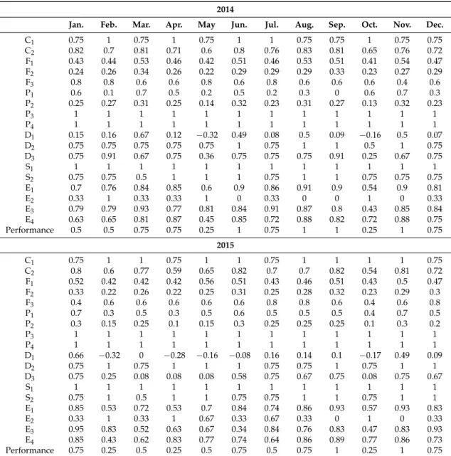
(2) Data pre-processing
The linear normalization functionyi = (xi−xmin)/(xmax−xmin)was used for the benefit indicators, andyi = (xmax−xi)/(xmax−xmin)was used for the cost indicators. Here,xiwas the original value of the indicators before normalization, andyiwas the value after normalization. The Valuesxmaxandxmin were the maximum and minimum values, respectively. To determinexmaxandxmin, these 18 indicators were also classified into two different types: qualitative and quantitative indicators. C1, P4, D2,
andS2 were qualitative indicators, while the others were quantitative indicators. The qualitative
indicators had to be digitized for further processing. In this paper, 0, 1, 2, 3, and 4 were used to express poor, reasonable, good, and excellent performance, respectively, for these four qualitative indicators. Theirxmaxandxminvalues were 4 and 0, respectively. For these quantitative indicators,xmaxandxmin were determined based on the company’s experience and their definitions; their values are presented in Table3. The normalized data were calculated and are presented in Table4.
Table 3.The values ofxmaxandxminfor the quantitative indicators.
C2 F1 F2 F3 P1 P2 P3 D1 D3 S1
(0, 2%) (0, 1) (0, 1) (100, 150) (85, 95) (0, 1) (0, 1) (0, 1) (100, 210) (0, 1)
Table 4.The processed data of Company F’s GSC over 24 months.
2014
Jan. Feb. Mar. Apr. May Jun. Jul. Aug. Sep. Oct. Nov. Dec.
C1 0.75 1 0.75 1 0.75 1 1 0.75 0.75 1 0.75 0.75
C2 0.82 0.7 0.81 0.71 0.6 0.8 0.76 0.83 0.81 0.65 0.76 0.72
F1 0.43 0.44 0.53 0.46 0.42 0.51 0.46 0.53 0.51 0.41 0.54 0.47
F2 0.24 0.26 0.34 0.26 0.22 0.29 0.29 0.29 0.33 0.23 0.27 0.29
F3 0.8 0.8 0.6 0.6 0.8 0.6 0.8 0.6 0.6 0.6 0.4 0.6
P1 0.6 0.1 0.7 0.5 0.2 0.5 0.2 0.3 0 0.6 0.7 0.3
P2 0.25 0.27 0.31 0.25 0.14 0.32 0.23 0.31 0.27 0.13 0.32 0.23
P3 1 1 1 1 1 1 1 1 1 1 1 1
P4 1 1 1 1 1 1 1 1 1 1 1 1
D1 0.15 0.16 0.67 0.12 −0.32 0.49 0.08 0.5 0.09 −0.16 0.5 0.07
D2 0.75 0.75 0.75 0.75 0.75 1 0.75 1 1 0.5 1 0.75
D3 0.75 0.91 0.67 0.75 0.36 0.75 0.75 0.75 0.91 0.25 0.67 0.75
S1 1 1 1 1 1 1 1 1 1 1 1 1
S2 0.75 0.75 0.5 1 1 1 0.75 1 1 0.75 0.75 0.75
E1 0.7 0.76 0.84 0.85 0.6 0.9 0.86 0.91 0.9 0.54 0.9 0.81
E2 0.33 1 0.33 0.33 1 0 0.33 0 0 1 0 0.33
E3 0.79 0.79 0.93 0.77 0.81 0.84 0.91 0.87 0.8 0.43 0.85 0.84
E4 0.63 0.65 0.81 0.87 0.45 0.85 0.72 0.88 0.82 0.72 0.88 0.75
Performance 0.5 0.5 0.75 0.75 0.25 1 0.75 1 1 0.25 1 0.75
2015
C1 0.75 1 1 0.75 1 1 0.75 1 1 1 1 0.75
C2 0.8 0.6 0.77 0.59 0.65 0.82 0.7 0.7 0.82 0.54 0.81 0.72
F1 0.52 0.42 0.42 0.42 0.56 0.51 0.43 0.46 0.51 0.43 0.5 0.47
F2 0.33 0.22 0.26 0.22 0.25 0.31 0.25 0.28 0.32 0.23 0.29 0.3
F3 0.4 0.6 0.6 0.6 0.6 0.6 0.8 0.8 0.6 0.4 0.6 0.8
P1 0.7 0.3 0.5 0.3 0.5 0.6 0.5 0.5 0.5 0.4 0.7 0.5
P2 0.3 0.15 0.25 0.1 0.15 0.3 0.25 0.25 0.25 0.1 0.3 0.2
P3 1 1 1 1 1 1 1 1 1 1 1 1
P4 1 1 1 1 1 1 1 1 1 1 1 1
D1 0.66 −0.32 0 −0.28 −0.16 −0.08 0.16 0.14 0.1 −0.17 0.49 0.09
D2 0.75 1 0.75 1 1 1 0.75 0.75 1 0.75 1 1
D3 0.75 0.25 0.08 0.08 0.08 0.58 0.75 0.67 0.75 0.08 0.75 0.67
S1 1 1 1 1 1 1 1 1 1 1 1 1
S2 0.75 1 0.5 1 1 0.75 0.75 1 1 0.75 1 1
E1 0.85 0.53 0.72 0.53 0.7 0.84 0.74 0.86 0.93 0.57 0.93 0.83
E2 0.33 1 0.33 1 0.67 0.33 0.67 0.33 0 1 0 0.33
E3 0.95 0.83 0.52 0.63 0.67 0.34 0.84 0.76 0.83 0.47 0.83 0.93
E4 0.85 0.43 0.62 0.83 0.77 0.74 0.64 0.86 0.89 0.77 0.86 0.73
7.2. Selection Indicators
In this paper, RS theory was used to remove the redundant evaluation indicators. The results analysis revealed that indicator F1 was redundant. Therefore, the data of F1 were removed, and the data of the selection indicators (i.e., the final input data for the proposed model) are in TableA1 (see AppendixA).
7.3. Chromosomal Gene Coding
The mapping relationships among the weight vectors and the threshold values of each layer and the chromosome code strings are shown in formula (8). In this formula, every code string represented a special shape of the neural network.
[wij][vki][θj][θk] (8)
In formula (8), the weights between the hidden and input layers arewij. The weights between the output and weights arewki. The parameters[θj]and[θk]are thejth neuron threshold of the hidden layer and thekth neuron threshold of the output layer, respectively.
7.4. Fitness Formula
In GA, the fitness formula is used to guide the search of the evaluation formula, and it is not constrained by the formula’s continuity or derivative. For a feedforward neural network, if the energy value of the error formula is small, then the network will have better performance. Therefore, the fitness formula is defined as formula (9).
F(x) = 1
E(s) (9)
7.5. Acquisition of the Hidden Layer Nodes
For a multilayer neural network, the number of the hidden layers should be determined first. A network containing at least one S-type hidden layer and one linear output layer can approach any rational number. The increase of the number of hidden layers strengthens the processing capacity of the neural network. If the training time of the network weights and the training sample numbers increase, the neural network will be more complicated. Therefore, a single hidden layer neural network was selected for use in this study. In the neural network, the S-style tansigfunction and the S-style logsig function were used as the transfer function of the hidden layer and output layer neurons, respectively.
During the modeling process of the neural network, the selection of the hidden nodes was important. If the hidden layer node was too high or too low, it would have a negative impact on the neural network. By reviewing the literature, a traversal method was selected to determine the node number in the hidden layer. The network included a different number of neurons in the hidden layer that would be trained and compared. When the network effect was optimal, the corresponding hidden node was the best node.
In this study, the initial number of nodes was set to zero, and then, the number of nodes was adjusted and the corresponding errors of these nodes were compared. By analyzing the results of this procedure, it was determined that when the node number was 20, the error (4.08×10⁻⁸) was
minimized. Therefore, the number of hidden nodes number was 20.
7.6. Application Process of the GA-LMBP Neural Network Algorithm Step 1: The topology of the neural network should be decided.
Step 2: The population Pop (N, L) and the algebratshould be initialized, and the fitness formula F(x)and the chromosome gene encoding should be set.
Step 4: Using the roulette selection method, conduct the selection operation. Using the arithmetic crossover, conduct the crossover operation to obtain the new individuals. Using the non-uniform mutation, conduct the mutation operation to obtain the new individuals.
Step 5: The optimal individual and the new individual should be retained, and then, the next generation will form.
Step 6: Determine whethert≥T; if yes, go to step 7. Otherwise, go to step 3.
Step 7: The best individual should be decoded. Then, the decoded values will be used as the initial weights and threshold values of the LMBP neural network. The values ofεandµshould be set.
Step 8: Train the LMBP neural network using the data in TableA1.
Step 9: The values ofokandE(s)should be calculated. IfE(s)<ε, then output the result and go to step 10. Otherwise, go to step 8.
Step 10: Output the result, end.
7.7. Results Analysis and Discussion
In TableA1, the “Performance” row presents the performance values of company F from 2014 to 2015. These data can be represented as follows:
dk = [0.5 0.5 0.75 0.75 0.25 1 0.75 1 1 0.25 1 0.75 0.75 0.25 0.50 0.25 0.50 0.75 0.50 0.75 1 0.25 1 0.75].
As noted in the previous discussion, in GA, the population size (55), the covariations’ coefficient (0.068), the evolution (500), and the cross coefficient value (0.75) were set. The node numbers of the input (17) and hidden layers (20) were obtained. The output layer node number was one. The standard of the MSE was 1× 10⁻². To evaluate the performance of the proposed algorithm, the BP neural
network algorithm was chosen and compared with the proposed model.
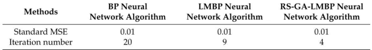
The results of the RS-GA-LMBP network are revealed that when the network of the RS-GA-LMBP neural network algorithm reached a stable state, the value of MSE was 4.03×10⁻⁴
and the number of iterations was 4. The results of the model output was ok, where,
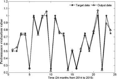
ok = [0.5213 0.5523 0.7312 0.7301 0.2647 0.9801 0.7300 0.9721 1.0623 0.2216 0.9642 0.7723 0.7201 0.2302 0.5179 0.2645 0.5340 0.7278 0.5346 0.7834 1.0756 0.2309 0.8909 0.7978]. To intuitively illustrate the prediction accuracy of the proposed model, the output values were compared with the target values, as shown in Figure3. Based on Figure3, it can be observed that the output and target values are basically consistent, indicating that the proposed model has a high prediction accuracy.
−
−
Figure 3.Comparison between target values and output values (using RS-GA-LMBP).
analysis was conducted, and the analysis results are shown in Figure4. TheX-axis indicates the target values, and theY-axis indicates the output values. The slope of the ideal regression curve is 1. In Figure4, the corresponding R (the fitness of the network) is 0.9889, which is close to 1, indicating that the proposed model has a good network performance.
−
−
Figure 4.Linear regression analysis of the outputs (using RS-GA-LMBP).
To explain the credibility and effectiveness of the proposed model, BP and LMBP neural network algorithms were used. The results of BP and LMBP neural network algorithms are shown as: (1) when the network of the BP neural network algorithm reached a stable state, the value of MSE was 6.73 × 10⁻⁴, and the number of iterations was 20; (2) when the
network of the LMBP neural network algorithm reached a stable state, the value of MSE was 5.63×10⁻⁴, and the number of iterations was 9. The output of BP model was o′
k, where, o′
k = [0.5213 0.5723 0.7062 0.6431 0.2947 0.9341 0.7121 0.9481 1.0723 0.2086 0.9542 0.7923 0.7081 0.2112 0.5579 0.2745 0.5540 0.7278 0.5546 0.7984 1.0856 0.2209 0.8700 0.8278]. The output of LMBP model was o′′
k, where, o ′′
k = [0.5321 0.5613 0.7134 0.6867 0.2801 0.9471 0.7211 1.031 0.9467 0.2845 1.0445 0.7867 0.7189 0.2245 0.5231 0.27 0.5437 0.7345 0.5437 0.7834 1.0801 0.2299 0.8623 0.8114].
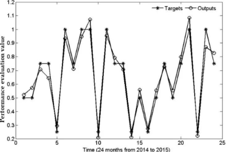
To intuitively illustrate the prediction accuracy of the BP neural network algorithm and the LMBP neural network algorithm, their output values were compared with the target values, as shown in Figures5and6. Based on Figure5, it can be observed that the consistency between output values and target values in the BP neural network algorithm was not as good as that in the proposed model. Based on Figure6, one can see that the consistency between output values and target values in the LMBP neural network algorithm was not as good as that in the proposed model.
−
−
.
Figure 6.Comparison between target values and output values (using LMBP).
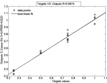
To further examine the performance of the BP network and the LMBP network after training, further simulation analysis was implemented based on the training results. According to the output and target values, a linear regression analysis was conducted, and the analysis results are shown in Figures7and8. TheX-axis indicates the target values, and theY-axis indicates the output values. In 0.9494, which is lower than 0.9889. In Figure8, the corresponding R (the fitness of the LMBP network) was 0.9676, which is lower than 0.9889. These indicate that the proposed model has a better network performance than that of the BP neural network algorithm and the LMBP neural network algorithm.
.
Figure 7.Linear regression analysis of outputs (using BP).
ThedTvalues represent the difference betweendkandok, andE= (dT)2/2.dT′represents the difference betweendkando′k, andE′ = (dT′)
2/2. By calculation, we obtain
E=10−2×[0.0227 0.1368
0.0177 0.0198 0.0108 0.0198 0.0200 0.0389 0.1941 0.0403 0.0641 0.0249 0.0447 0.0196 0.0160 0.0105 0.0578 0.0246 0.0599 0.0558 0.2858 0.0182 0.5951 0.1142],E′ = 10−2×[0.0227 0.2614 0.0999 0.2171 0.0959
0.5714 0.0718 0.1347 0.2614 0.0857 0.1049 0.0895 0.0878 0.0753 0.1676 0.0300 0.1458 0.0246 0.1491 0.1171 0.3664 0.0423 0.8450 0.3026], andE′′ =10−2×[0.0515 0.1879 0.067 0.2003 0.0453 0.1399 0.0418 0.048 0.142
E
E
E
E
E
E
E
E
Figure 8.Linear regression analysis of outputs (using LMBP).
To analyze the accuracy of the proposed model,E,E′, andE′′were compared, as shown in Figure9. In Figure9, it can be observed that the output of the proposed model is highly similar to that of the target data. InE, the maximum error was 0.5951%, and which is less than the 1% value that is accepted in GSC performance evaluation. This result shows that the proposed model can be used for GSC performance evaluation. This model is efficient, valid, and accurate. According to Figure9, it can also be observed that BP and LMBP neural network algorithms were also accurate for GSC performance evaluation. However, the maximum errors, inE′ (0.8450) andE′′ (0.6466), which are higher than 0.5951%, indicating that the BP network algorithm and the LMBP neural network algorithm were not as accurate as the proposed model.
E
E
E
Figure 9.Comparison betweenE,E′andE′′.Table 5.Performance analysis of the evaluation methods.
Methods BP Neural Network Algorithm
LMBP Neural Network Algorithm
RS-GA-LMBP Neural Network Algorithm
Standard MSE 0.01 0.01 0.01
Iteration number 20 9 4
8. Conclusions
In this paper, the methods and existing performance indicator systems for GSC performance evaluation were discussed. The applications and shortages of 5DBSC on GSC performance evaluation were discussed and an improved 5DBSC was proposed. Meanwhile, the applications and shortages of RS theory, GA, LMBP neural network algorithm, and GA-LMBP neural network algorithm on supply chain performance evaluation were analyzed. Then, a method was proposed. Finally, a case study was presented based on the new method. This study achieved the following:
(1) An improved 5DBSC for GSC performance evaluation was proposed. Based on the applications and shortcomings of the 5DBSC and the requirements of the IOS 14000 Environment Management Standard, the 5DBSC for GSC performance evaluation was improved. Its main contribution is that the measurement method of the “environmental pollution” indicator contained in the green performance was improved. The “environmental pollution” indicator was revised to measure the total emissions of “three wastes”. The modified indicator was more easily measured and more practical.
A suitable 5DBSC was proposed and the measurement methods of its indicators are more standardized and clear. This model provides a reference for building the normal indicator system for GSC performance evaluation.
(2) A new algorithm was proposed for GSC performance evaluation. According to the applications and shortcomings of RS theory, GA, the LMBP neural network algorithm, and the GA-LMBP neural network algorithm for evaluating supply chain performance, a RS-GA-LMBP neural network algorithm was proposed and developed. The algorithm of the proposed model was presented. Then, from the aspect of a theoretical analysis and a literature review, it was demonstrated that the proposed algorithm could be used in an uncertain environment and could help eliminate redundant indicators. This algorithm has a high convergence speed and a more accurate prediction ability.
Thus, a new algorithm was proposed that has a high data processing speed and a more accurate prediction ability. This algorithm suits the uncertain environment well. In theory, the algorithm is an optimized method that can be utilized for the performance evaluation of a company and is a new development in GSC performance evaluation theory.
(3) From a practical perspective, the effectiveness of the proposed algorithm was confirmed. A case study was conducted, and the practical values of 18 indicators from 2014 to 2015 were collected from automotive company F. According to the analysis, the results show that the proposed model is effective, valid, and reliable. This model has a faster convergence speed than BP and LMBP neural network algorithms.
The proposed model has a practical value for GSC performance evaluation. It has a faster convergence speed and more accurate predictive capability.
5DBSC system, RS theory, the LMBP neural network algorithm, and GA. This method can not only accurately evaluate the level of GSC performance but also provide solutions to optimize and improve GSC performance.
From a practical perspective, the proposed method was implemented based on a case study. By optimizing the performance of the supply chain core enterprise, the purpose that performance evaluation methods could guide business practices could achieved. In this way, the operational efficiency and effectiveness of the supply chain can be enhanced, and the supply chain performance can be fully enhanced.
However, there are some limitations. Firstly, it should be pointed out that the model is only based on 24 months’ data from company F. To make the model more reliable, more data should be collected to train the network. Meanwhile, the proposed method was only tested on company F. To prove its reliability, more firms’ data should be collected and used.
In the future, more data from different enterprises or industries should be used to confirm the credibility and effectiveness of the proposed model. Meanwhile, the proposed model can also be used in the performance evaluation of other areas.
Acknowledgments: The authors thank the editors and anonymous referees who commented on this article. The authors also thank Shuping Yi for his valuable comments and suggestions. This research was supported by the Youth Science Foundation of China.
Author Contributions:Pan Liu and Shuping Yi conceived, designed, and performed the experiments; Pan Liu analyzed the data and wrote the paper.
Conflicts of Interest:The authors declare that there is no conflict of interest. Appendix A
Table A1.The data of the selection indicators.
2014
Jan. Feb. Mar. Apr. May Jun. Jul. Aug. Sep. Oct. Nov. Dec.
C1 0.75 1 0.75 1 0.75 1 1 0.75 0.75 1 0.75 0.75
C2 0.82 0.7 0.81 0.71 0.6 0.8 0.76 0.83 0.81 0.65 0.76 0.72
F2 0.24 0.26 0.34 0.26 0.22 0.29 0.29 0.29 0.33 0.23 0.27 0.29
F3 0.8 0.8 0.6 0.6 0.8 0.6 0.8 0.6 0.6 0.6 0.4 0.6
P1 0.6 0.1 0.7 0.5 0.2 0.5 0.2 0.3 0 0.6 0.7 0.3
P2 0.25 0.27 0.31 0.25 0.14 0.32 0.23 0.31 0.27 0.13 0.32 0.23
P3 1 1 1 1 1 1 1 1 1 1 1 1
P4 1 1 1 1 1 1 1 1 1 1 1 1
D1 0.15 0.16 0.67 0.12 −0.32 0.49 0.08 0.5 0.09 −0.16 0.5 0.07
D2 0.75 0.75 0.75 0.75 0.75 1 0.75 1 1 0.5 1 0.75
D3 0.75 0.91 0.67 0.75 0.36 0.75 0.75 0.75 0.91 0.25 0.67 0.75
S1 1 1 1 1 1 1 1 1 1 1 1 1
S2 0.75 0.75 0.5 1 1 1 0.75 1 1 0.75 0.75 0.75
E1 0.7 0.76 0.84 0.85 0.6 0.9 0.86 0.91 0.9 0.54 0.9 0.81
E2 0.33 1 0.33 0.33 1 0 0.33 0 0 1 0 0.33
E3 0.79 0.79 0.93 0.77 0.81 0.84 0.91 0.87 0.8 0.43 0.85 0.84
E4 0.63 0.65 0.81 0.87 0.45 0.85 0.72 0.88 0.82 0.72 0.88 0.75
Performance 0.5 0.5 0.75 0.75 0.25 1 0.75 1 1 0.25 1 0.75
2015
C1 0.75 1 1 0.75 1 1 0.75 1 1 1 1 0.75
C2 0.8 0.6 0.77 0.59 0.65 0.82 0.7 0.7 0.82 0.54 0.81 0.72
F2 0.33 0.22 0.26 0.22 0.25 0.31 0.25 0.28 0.32 0.23 0.29 0.3
F3 0.4 0.6 0.6 0.6 0.6 0.6 0.8 0.8 0.6 0.4 0.6 0.8
P1 0.7 0.3 0.5 0.3 0.5 0.6 0.5 0.5 0.5 0.4 0.7 0.5
P2 0.3 0.15 0.25 0.1 0.15 0.3 0.25 0.25 0.25 0.1 0.3 0.2
P3 1 1 1 1 1 1 1 1 1 1 1 1
Table A1.Cont.
2015
D1 0.66 −0.32 0 −0.28 −0.16 −0.08 0.16 0.14 0.1 −0.17 0.49 0.09
D2 0.75 1 0.75 1 1 1 0.75 0.75 1 0.75 1 1
D3 0.75 0.25 0.08 0.08 0.08 0.58 0.75 0.67 0.75 0.08 0.75 0.67
S1 1 1 1 1 1 1 1 1 1 1 1 1
S2 0.75 1 0.5 1 1 0.75 0.75 1 1 0.75 1 1
E1 0.85 0.53 0.72 0.53 0.7 0.84 0.74 0.86 0.93 0.57 0.93 0.83
E2 0.33 1 0.33 1 0.67 0.33 0.67 0.33 0 1 0 0.33
E3 0.95 0.83 0.52 0.63 0.67 0.34 0.84 0.76 0.83 0.47 0.83 0.93
E4 0.85 0.43 0.62 0.83 0.77 0.74 0.64 0.86 0.89 0.77 0.86 0.73
Performance 0.75 0.25 0.5 0.25 0.5 0.75 0.5 0.75 1 0.25 1 0.75
References
1. Srivastava, S.K. Green supply-chain management: A state-of-the-art literature review.Int. J. Manag. Rev.
2007,9, 53–80. [CrossRef]
2. Carter, C.R.; Rogers, D.S. A framework of sustainable supply chain management: Moving toward new theory.Int. J. Phys. Distrib. Logist. Manag.2008,38, 360–387. [CrossRef]
3. Weng, H.-H.R.; Chen, J.-S.; Chen, P.-C. Effects of green innovation on environmental and corporate performance: A stakehold perspect.Sustainability2015,7, 4997–5026. [CrossRef]
4. Bhattacharya, A.; Mohapatra, P.; Kumar, V.; Dey, P.K.; Brady, M.; Tiwari, M.K.; Nudurupati, S.S. Green supply chain performance measurement using fuzzy ANP-based balanced scorecard: A collaborative decision-making approach.Prod. Plan. Control2014,25, 698–714. [CrossRef]
5. Hervani, A.A.; Helms, M.M.; Sarkis, J. Performance measurement for green supply chain management.
Benchmarking2005,12, 330–353. [CrossRef]
6. Shen, L.; Olfat, L.; Govindan, K.; Khodaverdi, R.; Diabat, A. A fuzzy multi criteria approach for evaluating green supplier’s performance in green supply chain with linguistic preferences.Resour. Conserv. Recycl.2013,
74, 170–179. [CrossRef]
7. Uygun, Ö.; Dede, A. Performance evaluation of green supply chain management using integrated fuzzy multi-criteria decision making techniques.Comput. Ind. Eng.2016, in press. [CrossRef]
8. Richardson, P. Fitness for the Future: Applying Biomimetics to Business Strategy. Ph.D. Thesis, Bath University, Bath, UK, 2010.
9. Li, Y. Application of GA and SVM to the performance evaluation of supply chain.Comput. Eng. Appl.2010,
46, 246–248.
10. Fan, X.; Zhang, S.; Wang, L.; Yang, Y.; Hapeshi, K. An evaluation model of supply chain performances using 5DBSC and LMBP neural network algorithm.J. Bionic Eng.2013,10, 383–395. [CrossRef]
11. Xi, Y.F.; Wang, C.; Nie, X.X. Study of the evaluation methods of supply chain performances using fuzzy neural network.Inf. J.2007,9, 77–79.
12. Seeley, T.D.The Wisdom of the Hive: The Social Physiology of Honey Bee Colonies; Harvard University Press: Cambridge, UK, 1996.
13. Martens, D.; De Backer, M.; Haesen, R.; Vanthienen, J.; Snoeck, M.; Baesens, B. Classification with ant colony optimization.IEEE Trans. Evol. Comput.2007,11, 651–665. [CrossRef]
14. Gabbert, P.; Brown, D.E.; Huntley, C.L.; Markowicz, B.P.; Sappington, D.E. A system for learning routes and schedules with genetic algorithms. In Proceedings of the Fourth International Conference on Genetic Algorithms (ICGA’91), Santt Diego, CA, USA, 13–16 July 1991; pp. 430–436.
15. Huang, H.X. Modeling and prediction of water-assisted injection molding based on GA-LMBP inverse neural network.J. South China Univ. Technol. Nat. Sci. Ed.2007,35, 23–27.
16. Wu, X.; Xie, L.; Ge, M. Analog circuit fault diagnosis method based on GA-LMBP.Mod. Electron. Tech.2010,
4, 177–189.
18. Xue, Y.Research on Evaluation and Analysis of Passenger Comfort in Relation to Vibration in Railway Vehiele; Beijing Jiaotong University: Beijing, China, 2011.
19. Zhu, Q.; Sarkis, J. Relationships between operational practices and performance among early adopters of green supply chain management practices in Chinese manufacturing enterprises.J. Oper. Manag.2004,22, 265–289. [CrossRef]
20. Tseng, M.L.; Chiu, A.S.F. Evaluating firm’s green supply chain management in linguistic preferences.
J. Clean. Prod.2013,40, 22–31. [CrossRef]
21. Tseng, M.L.; Chiang, J.H.; Lan, L.W. Selection of optimal supplier in supply chain management strategy with analytic network process and choquet integral.Comput. Ind. Eng.2009,57, 330–340. [CrossRef]
22. Sarkis, J. A strategic decision framework for green supply chain management. J. Clean. Prod. 2003,11, 397–409. [CrossRef]
23. Zhu, Q.; Sarkis, J.; Geng, Y. Green supply chain management in china: Pressures, practices and performance.
Int. J. Oper. Prod. Manag.2005,25, 449–468. [CrossRef]
24. Diabat, A.; Govindan, K. An analysis of the drivers affecting the implementation of green supply chain management.Resour. Conserv. Recycl.2011,55, 659–667. [CrossRef]
25. Tseng, M.L.; Lin, Y.H.; Tan, K.; Chen, R.H.; Chen, Y.H. Using TODIM to evaluate green supply chain practices under uncertainty.Appl. Math. Model.2014,38, 2983–2995. [CrossRef]
26. Beamon, B.M. Measuring supply chain performance.Int. J. Oper. Prod. Manag.1999,19, 275–292. [CrossRef] 27. Farris, P.W.; Bendle, N.T.; Pfeifer, P.E.; Reibstein, D.J.Marketing Metrics: The Definitive Guide to Measuring
Marketing Performance; Pearson Education: Upper Saddle River, NJ, USA, 2010.
28. Stewart, G. Supply-chain operations reference model (SCOR): The first cross-industry framework for integrated supply-chain management.Logist. Inf. Manag.1997,10, 62–67. [CrossRef]
29. Yi, K.G. KPI assessment: Study of implication, workflow and counter measures.Technol. Econ. 2005,24, 48–49.
30. Gecevska, V.; Chiabert, P.; Anisic, Z.; Lombardi, F. Product lifecycle management through innovative and competitive business environment.J. Ind. Eng. Manag.2010,3, 323–336. [CrossRef]
31. Alemanni, M.; Alessia, G.; Tornincasa, S.; Vezzetti, E. Key performance indicators for PLM benefits evaluation: The Alcatel Alenia Space case study.Comput. Ind.2008,59, 833–841. [CrossRef]
32. Kaplan, R.S.; Norton, D.P. The balanced scorecard: Measures that drive performance.Harv. Bus. Rev.1992,
70, 71–79. [PubMed]
33. Wong, W.P. A review on benchmarking of supply chain performance measures.Benchmarking2008,15, 25–51. [CrossRef]
34. Akkermans, H.; Orschot, K.V. Developing a balanced scorecard with system dynamics. In Proceedings of the 20th International System Dynamics Conference, Palermo, Italy, 28 July–1 August 2002.
35. Zheng, P. Study of Methods for Evaluating the Performance of Dynamic Supply Chains. Ph.D. Thesis, Hunan University, Changsha, China, 2008.
36. Kurnia, S.; Shokravi, S. A step towards developing a sustainability performance measure within industrial networks.Sustainability2014,6, 2201–2222.
37. Seuring, S.; Müller, M. From a literature review to a conceptual framework for sustainable supply chain management.J. Clean. Prod.2008,16, 1699–1710. [CrossRef]
38. Duarte, S.; Cruz-Machado, V.A. Lean and green supply chain performance: A balanced scorecard perspective. InProceedings of the Eighth International Conference on Management Science and Engineering Management; Springer: Heidelberg, Germany, 2014.
39. Shao, K.; Yang, J. Study on the performance evaluation of green supply chain Based on the balance scorecard and fuzzy theory. In Proceedings of the 2nd IEEE International Conference on Information Management and Engineering (ICIME), Chengdu, China, 16–18 April 2010; pp. 242–246.
40. Chen, W.W.; Zhang, Y.N.; Ouyang, H.X. Green building supply chain performance evaluation based on improved BSC method.J. Eng. Manag.2014,28, 201403007.
41. Fukushima, K. Neocognitron: A self-organizing neural network model for a mechanism of pattern recognition unaffected by shift in position.Biol. Cybern.1980,36, 193–202. [CrossRef] [PubMed]
43. Mcculloch, W.; Pitts, W. A logical calculus of the ideas immanent in nervous activity.Bull. Math. Biophys.
1943,5, 115–133. [CrossRef]
44. Zhang, F.M.; Cao, Q.K.; Fang, Q.Y. A comparative inquiry into supply chain performance appraisal based on support vector machine and neural network. In Proceedings of the 2008 International Conference on Management Science & Engineering, Long Beach, CA, USA, 10–12 September 2008; pp. 370–377.
45. Bocharnikov, Y.V.; Tobias, A.M.; Roberts, C. Reduction of train and net energy consumption using genetic algorithms for Trajectory Optimisation. In Proceedings of the IET Conference on Railway Traction Systems, Birmingham, UK, 13–15 April 2010; pp. 1–5.
46. Cha, S.H.; Tappert, C.C. A genetic algorithm for constructing compact binary decision trees. J. Pattern Recognit. Res.2009,4, 1–13. [CrossRef]
47. Shi, C.D.; Chen, J.H. Study of supply chain performance prediction based on rough sets and BP neural network.Comput. Eng. Appl.2006,43, 203–205.
48. Zheng, P.; Lai, K.K. A rough set approach on supply chain dynamic performance measurement. InKes International Conference on Agent and Multi-Agent Systems: Technologies and Applications; Springer: Heidelberg, Germany, 2008; Volume 4953, pp. 312–322.
49. Huang, J.Y.H.J.Z. BP network and its application in SCM performance evaluation.Shanghai Manag. Sci.2006,
6, 57–75.
50. Pawlak, Z. Rough set.Int. J. Comput. Inf. Sci.1982,11, 341–356. [CrossRef]
51. Xu, J.; Li, B.; Wu, D. Rough data envelopment analysis and its application to supply chain performance evaluation.Int. J. Prod. Econ.2009,122, 628–638. [CrossRef]
52. Dong, X.U.; Chen, C.X.; Wang, H.H. Research on heart disease diagnosis basd on RS-LMBP neural network.
Comput. Simul.2011,28, 236–239.
53. Øhrn, A.; Komorowski, J. Rosetta—A rough set toolkit for analysis of data. In Proceedings of the Third International Joint Conference on Information Sciences, Durham, NC, USA, 1–5 March 1997; pp. 403–407.
54. Øhrn, A.; Komorowski, J.; Skowron, A.; Synak, P. The Design and Implementation of a Knowledge Discovery Toolkit Based on Rough Sets—The ROSETTA System. Available online: https://www.researchgate.net/publication/2806936_The_Design_and_Implementation_of_a_Knowledge_ Discovery_Toolkit_Based_on_Rough_Sets_-_The_ROSETTA_System (accessed on 28 May 2016).
55. The ROSETTA WWW Homepage. Available online: http://www.idi.ntnu.no/~aleks/ROSETTA/ (accessed on 28 May 2016).