S P I R I T: Satisfiability Problem Implementation for Redundancy
Identification and Test Generation
1Emil Gizdarski*2 and Hideo Fujiwara**
* Department of Computer Systems, University of Rousse, 7017 Rousse, Bulgaria
** Nara Institute of Science and Technology, Ikoma, Nara 630-0101, Japan E-mail: [email protected], [email protected]
1 This work was supported in part by JSPS under grant P99747 and in part by
Semiconductor Technology Academic Research Center (STARC) under the Research Project (No. 973).
2 Currently visiting at Nara Institute of Science and Technology
Abstract. In this paper an efficient test pattern generation (TPG) algorithm for combinational circuits based on the Boolean satisfiability method (SAT) is presented. We examine some not so popular approaches as a single cone processing, single path oriented propagation and backward justification. We give a new definition for SAT-based test generation and present duality of learning phenomenon. The resultant ATPG system, called SPIRIT, combines the flexibility of SAT- based TPG algorithms with the efficiency of structural TPG algorithms. Experimental results demonstrate the efficiency and robustness of the proposed TPG algorithm. Without fault simulation, SPIRIT is able to generates complete test sets for the ISCAS‘85 benchmark circuits and full scan version of the ISCAS‘89 benchmark circuits within 3 minutes on a 450MHz Pentium-III PC.
1. Introduction
In recent years substantial progress has been achieved in the fields of design automation, verification and test generation for integrated circuits using the Boolean satisfiability method. Although there are many effective TPG algorithms, their performance is decreasing because of the increase in size and complexity of integrated circuits. This problem motivates us to work on the well- studied topic - test generation for combinational circuits. The goal is to increase efficiency and robustness of TPG algorithms. To do so, we study the well-known and the most successful ATPG systems: (structural) PODEM[6], FAN[7], SOCRATES[18], [22] and ATOM[8] (algebraic) Nemesis[13], TRAN[3] and TEGUS[19], and (mixed) TIP[10,20]. Many techniques to increase efficiency of TPG algorithms have been proposed in the past two
decades. The most important of them implemented in our TPG algorithm are briefly described below:
- An unjustified line [7] is an efficient concept for justification and an early detection of inconsistency.
- 9-V[16] and 16-V[17] algebra allows more precise value assignment and search space reduction.
- Static learning [18] is introduced as a preprocessing phase that performs iterative both value assignments (0 and 1) through the variables and finds new dependencies (global implications) between signals.
- Recursive learning [12] is the first complete learning procedure able to find all implications (necessary assignments) at the current level of the decision tree by recursive AND-OR search on the unjustified lines.
- The Boolean satisfiability method gives an elegant formulation of TPG problem [13]. Until this time, the decision points of branch and bound search were limited to the primary inputs [6], head lines [7] or implying nodes [21]. Actually, the Boolean satisfiability method translates TPG problem to a characteristic formula that includes all signals of the circuit. This increases the degree of freedom for TPG algorithms.
- Single Path Oriented Propagation (SPOP) [10] simplify propagation (for structural TPG algorithms) and reduces the need for extracting structural constraints (for SAT-based TPG algorithms).
- Single cone processing [14] reduces the size of problem and allows more effective application of unique sensitization [7].
- Backward justification [11] as an alternative of PODEM algorithm [6].
- A new data structure of the complete implication graph that simplifies deriving of global ∧-implications [4] as an alternative of the complete graph used in [10,20]. IEEE the 9th Asian Test Symposium (ATS 2000), pp. 171-178, Dec. 2000.
The resultant ATPG system called SPIRIT (Satisfiability Problem Implementation for Redundancy Identification and Test generation) combines simplicity, efficiency and robustness.
The rest of the paper is organized as follows. In Section 2, a systems overview is provided. In Section 3, a new definition of SAT based TPG algorithm is presented. In Section 4, a static learning procedure is presented. In Section 5, a propagation procedure is presented. In Section 6, a backward justification procedure and duality of learning phenomenon are presented. Section 7 provides experimental results and Section 8 concludes the paper.
2. System overview
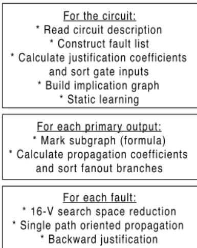
The phases for the proposed ATPG system are shown in Figure 1. Phase 1 (circuit preprocessing) reads a circuit description, constructs a collapsed fault list, calculates justification coefficients, builds an implication graph and performs static learning. Phase 2 (cone preprocessing) marks a characteristic formula corresponding to a single cone (primary output) and calculates fault propagation coefficients. Phase 3 (test session) performs 16-V search space reduction, propagation and justification.
In contrast to the most typical SAT-based TPG algorithms [3,13,19], SPIRIT builds the complete implication graph (formula) and performs static learning once for the whole circuit since static learning is prominent and time consuming step. Using SPOP, we also avoid the extracting structural constraints (D-chain conditions) [3,13,19]. This approach reduces considerably the preprocessing time but makes the resultant TPG algorithm unfeasible for redundancy removal because by removing redundant elements, the processed circuit is changed during test generation. In this way, some global implications found during static learning become invalid.
This disadvantage is not critical because the best results for redundancy removal can be achieved by resynthesis.
Using a single cone processing, we apply “Divide and Conquer” strategy. This approach may produce more that one test session for a redundant fault and even a detectable fault because SPIRIT has to prove that the fault is undetectable in respect to each primary output where the fault effect can be observed. On the other hand, this approach allows more effective application of 16-V search space reduction, the SPOP approach and backward justification.
3. SAT basis
The typical SAT-based algorithms [3,13,19] translate a problem into a characteristic formula that represents both the logical and structural constraints for the possible solutions. The characteristic formula is usually written in Conjunctive Normal Form (CNF) where one sum is called a clause. Clauses with one, two, three or more variables are called unary, binary, ternary and k-nary clauses respectively.
A CNF formula is represented by an implication graph. More formally, each variable X is represented by two nodes in the implication graph labeled X and X . Next, each binary clause (X ∨ Y) is viewed by two local implications ( X → Y) and ( Y → X) between these nodes, i.e., for each binary clause (X ∨ Y) there are two directed edges in the implication graph that represent these two local implications. A complete implication graph represents each k-nary clause by 2k ∧-nodes, k local
∧-implications and k-bit key dynamically calculated by the binding procedure [4]. An example is shown in Fugure2.
Since each k-nary clause corresponds to a logic gate then the following definitions can be used:
Definition 1: A k-nary clause is called unsatisfied iff it does not evaluate to 1. A clause is satisfied iff a variable in this clause is set to a value so that this clause evaluates to 1.
Definition 2: A k-nary clause is called unjustified line iff it is unsatisfied and the variable corresponding to the output of logic gate is specified (the least significant bit of the k-bit key is 1). A clause is satisfied iff an unspecified variable in this clause is set to a value so that this clause evaluates to 1.
Figure 1. SPIRIT flowchart
Figure 2. The representation of local ∧-implications For the circuit:
* Read circuit description
* Construct fault list
* Calculate justification coefficients and sort gate inputs
* Build implication graph
* Static learning For each primary output:
* Mark subgraph (formula)
* Calculate propagation coefficients and sort fanout branches
For each fault:
* 16-V search space reduction
* Single path oriented propagation
* Backward justification
A = 0 1 1 1 1 1 0 1 0 1 1 0 0 0 1 1 0 1 0 0 0 1 0 0 0
CONFLICT
INITIALIZATION B = 0
C = 1
A B C
(A∨B∨C ) A B
C
Since a test pattern for a fault is an input vector that sensitizes the fault and propagates the fault effect to a primary output, hereafter we will consider that:
• a test pattern is found iff both the fault under consideration and propagation path are sensitized and all unjustified lines are justified
If one of these conditions cannot be satisfied, the fault under consideration is proved as an undetectable in respect to the current primary output. In this way, we eliminate the deriving of structural constrains and simplify satisfying the logical constrains for test generation.
4. Static learning
Contrary to local implications that can be extracted by the structure of a circuit, detection of global implications requires a special analysis of the logic functions as they represent information that is not obvious from the circuit description. To find global implications, the static learning procedure iterates though the variables of the formula performing both value assignments (0 and 1) until one full iteration produces no new implications [19]. The derived global implications by static learning play an important role in avoiding a backtracking during branch and bound search (satisfying a CNF formula).
The leading static learning procedures [7,18] can find a limited number of global implications. In [18] static learning is performed as a preprocessing phase based on contradiction, Equation (1), where A,B∈{0,1}.
(X=A → Y=B) ⇔ (Y= B → X= A ) (1)
Clearly, the 2CNF portion of a CNF formula (only the binary clauses) fulfills priory the law of contraposition. This is not true when the k-nary clauses are also included. For example, it is possible that an assignment sets k-1 variables in a k-nary clause and the clause is still unsatisfied. In this case, the last variable should be set to a logic value so that this clause is satisfied. If the last variable of this clause is an output (or input) of the corresponding gate, this binding rule is called a forward (or backward) local ∧-implication.
Since the deriving of each new global implication involved at least one forward or backward ∧-implication (the least significant bit of k-bit key is 0 or 1 respectively), we will consider that the type of this ∧-implication determines the type of the derived global implication.
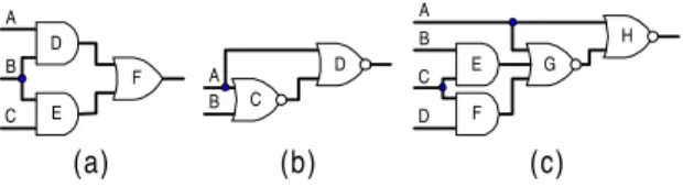
For the circuit in Figure 3(a), a value assignment B=0 sets variables D and E to 0 and a ternary clause (D ∨ E ∨ F ) is still unsatisfied. To satisfy this clause, the binding procedure performs a forward local ∧-implication and sets the last unspecified variable F to 0. Thus, backward global implication (F=1 → B=1) is found by contradiction.
For the circuit in Figure 3(b), a value assignment D=1 sets variables A and C to 0, and a ternary clause (A ∨ B ∨ C) is still unsatisfied. To satisfy this clause, the binding procedure performs a backward local ∧-implication and sets variable B to 1. Thus, forward global implication (B=0 → D=0) is found by contradiction.
Using unjustified lines [7], some implications can be found as an intersection of the conditions for satisfying a k-nary clause. For the circuit in Figure 3(c), a value assignment H=1 sets variables A and G to 0 and a k-nary clause (A ∨ E ∨ F ∨ G) is still unsatisfied. To satisfy this clause either variable E or variable F must be set to 1, but each one of these value assignments implies that variable C should be set to 1. Therefore C=1 is a necessary assignment and backward global implication (H=1 → C=1) is found. Clearly, this global implication cannot be found by contradiction. This global implication can be easily found by deriving and performing global ∧- implications during static learning [4]. In [4], we also showed that some static global ∧-implications derived during static learning can be transformed without spare operations to dynamic implications during branch and bound search.
5. Single path oriented propagation
The SPOP approach has been introduced in [10]. Beginning from the fault location forward to the primary output, SPOP sensitizes path-segment by path-segment where a path-segment is defined as a subpath starting at the fault location or a fanout branch and ending at a fanout stem or the primary output. For the SPOP approach, the fanout stems are decision points and next path-segment is selected by initial sorting of the fanout branches using propagation coefficients (see Figure 1). In this way, the SPOP approach is an alternative to the D- frontier (for the structural TPG algorithms) and the extracting structural constraints (for the SAT-based TPG algorithms). The main advantage of the SPOP approach is that first it sensitizes the easiest path for fault effect propagation according to the selected criteria. In contrast, the alternative solutions can block the shortest propagation path by justification of the current path- segment. The disadvantage of the SPOP approach is that the number of unjustified lines increase considerably and it is possible that the sensitized propagation path is unjustifiable. We reduce these cases using static learning, Figure 3. Network examples 1, 2 and 3
(a) (c)
A
G H E
F B
D D
E F A
B
C
C
(b)
A
B C
D
16-V search space reduction and propagation path pruning techniques.
16-V search space reduction (SSR) is performed as a test session preprocessing phase. SSR starts from the fault location forward to the primary output, and calculates the possible assignments in a set of {0,1,D, D } for each variable in the CNF formula. SSR also takes into account the number of the propagation paths and reduces values {0,1} when only one propagation path is possible. Using observable points, some propagation paths can be reduced and even the CNF formula can be proved as unsatisfiable during SSR. For example, if a propagation path includes a line that is directly observable for another primary output, then the values {D, D } for the corresponding variable and all propagation paths that include this line can be reduced. If the set of possible value assignments of a variable is empty then the CNF formula is proved as unsatisfiable without propagation and justification. In this way, SSR specifies the logical constraints for a test session and also validates some global implications for the faulty circuit. However, both static learning and SSR do not guarantee that a sensitized propagation path is justifiable. It is possible that a sensitized propagation path cannot be justified. We reduce the number of the sensitized unjustifiable propagation paths using a propagation path pruning technique.
Propagation path pruning (PPP) is performed after the first sensitized propagation path is proved as unjustifiable. PPP checks each unjustified line by first level recursive learning. If an unjustifiable line is found then the PPP backtracks path segment by path segment to the highest level of SPOP where this line can be justified.
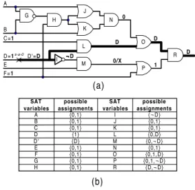
Example 1: Let us consider a s-a-0 fault at line D in Figure 4(a). Figure 4(b) shows the possible value assignments for each variable after SSR. Let D’-L-O-R be the first sensitized propagation path. In this case, N is unjustifiable line. If R is not a primary output that can produce sensitization of many propagation paths until the alternative path segment, D’-I-M-P-R is sensitized. This particular case can be avoided by static learning. For example, if static learning is performed then four global implications will be found: (F=1→J=1), (F=1→K=1), (N=0→H=0) and (R=0→H=0). These new implications find inconsistency by assignment O=D during SPOP. In the few cases when the global implications derived by static learning are not enough, PPP can also reduce the number of the sensitized unjustifiable propagation paths.
6. Justification and duality of learning Justification is performed after a propagation path is sensitized and has to justify all unjustified lines. We assume that a test pattern is found when a fault effect is propagated to the primary output and all unjustified lines are justified. In contrast, many SAT-based TPG algorithms try to satisfy all clauses in the CNF formula. This approach can produce a massive backtracking and even aborting after a test pattern is found. This approach also increases the number of specified primary inputs.
The backward justification procedure is based on justification coefficients calculated during circuit preprocessing (see Figure 1). The justification coefficients take into account the structure of the circuit and measure the relative difficulty for justification of each line in the circuit. By sorting the inputs of each logic gate using the justification coefficients, we suppose that each unjustified line can be justified by assigning a certain/controlling value to the first unspecified variable/input of the corresponding k-nary clause/gate.
During the SPOP phase all unjustified lines are included in a justification list which is sorted in an increasing order of justification coefficients before backward justification (heuristic BJ1). During backward justification this list is dynamically updated by adding new unjustified lines at the end of the list when the unjustified lines are processed (justified) starting from the end to the beginning of the justification list. Actually, this is a dynamic reordering of the variables based on a depth first search strategy. This strategy is more efficient than static order typical for the SAT-based TPG algorithms [3,13,19]. If a backtrack limit is exceeded, the backward justification is applied with the reverse ordered justification list (heuristic BJ2). In case that both these heuristics cannot justify or prove unjustifiable the sensitized propagation path, the backward justification performs heuristics BJ1* and BJ2* using dynamic learning (first level recursive learning).
Figure 4. Network example 4
{D} {0,1}
{1} possible assignments
{D,¬D} {0,1, ¬D}
{0,1, D} {0,¬D} {0,D} {0,1} possible assignments
H G F E D' D C B A SAT variables
R P O N M L K J I SAT variables
{0,1} {0,1}
{0,1} {0,1} {0,1} {0,1}
{¬D} {0,1}
{0,1}
(b)
R D
1 D N
D
0/X 0
O
P
(a)
K J
L
M
¬
¬
¬¬D H
s-a-0 D'=D I B
A
C =1
D =1 E F = 1
G
Example 2: Let us consider a s-a-0 fault at line C in Figure 5. During static learning four global implications are found: forward implications (B=0→J=0) and (F=0→K=0) and backward implications (M=1→J=0) and (N=0→K=0). After value assignment C’=D, the fault effect is propagated to the primary output and the values of signals are shown in Figure 5. As a result, four primary inputs are specified and two unjustified lines, J and K, are included in the justification list. During justification, variables A and E are set to 1 in order to justify lines J and K, i.e., in this case (case A), all primary inputs are specified. However, primary inputs A and E can be left unspecified because both unjustified lines J and K are already justified (case B).
Let us consider the same example without static learning. In this case (case C), variable K will be unspecified after SPOP since in Example 2 variable K is set to 0 by forward global implication (F=0→K=0). Next, the justification list will include lines J and L. To justify these unjustified lines, variables A and D should be set to 1. In this way without static learning, primary input E will be left unspecified. In summary, three solutions for justification are possible: (A) all variable are specified, (B) variables A and E are unspecified and (C) variable E is unspecified. If the circuit under consideration is a subcircuit of large circuit, each solution will produce different number of unjustified lines that have to be justified. This phenomenon is called here duality of learning. Obviously, static learning is important to decrease the number of backtracks. On the other hand, static learning may produce some spare unjustified lines that have to be justified.
Example 3: Let us consider again the circuit in Figure 3(b). Without static learning after assignment B=0, ternary clause (A∨B∨C) is still unsatisfied. To satisfy this clause either variable A or variable C should be set to 1 but both these value assignments set variable D to 0 therefore D=0 is a necessary assignment. If we apply this new dynamic forward implication derived by first level recursive learning then a new spare unjustified line D will be included into justification list.
Getting an idea of these examples to avoid spare unjustified lines (overspecification):
• all static forward global implications and ∧- implications as well as all dynamic forward implications must be discarded
In our justification procedure, we avoid overspecification by removing all forward global implications and ∧-implications after static learning as well as by restricting dynamic learning to the unjustified lines in the justification list.
7. Experimental results
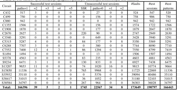
We implemented the presented TPG algorithm in ATPG system SPIRIT [5] and ran experiments on the ISCAS’85[1] benchmark circuits and full scan version of the ISCAS’89[2] benchmark circuits on a 450 MHz Pentium-III PC. For all experiments, the maximum number of both the sensitized unjustifiable paths during propagation and the backtracks during justification was set at 10. As a result, without fault simulation SPIRIT was able to generate complete test set and prove all redundant faults in the ISCAS’85 and ISCAS’89 benchmark circuits. Table 1 presents the number of the sensitized propagation paths for successful and unsuccessful test sessions (test patterns exist/does not exist). Accordingly, 99.97% of the successful test sessions generated test patterns by justification of the first sensitized propagation path. Also, 99.83% of the unsuccessful test sessions were identified during SSR or SPOP, i.e., without justification. Only 89 test sessions (0.05%) sensitized one or more unjustifiable propagation paths.
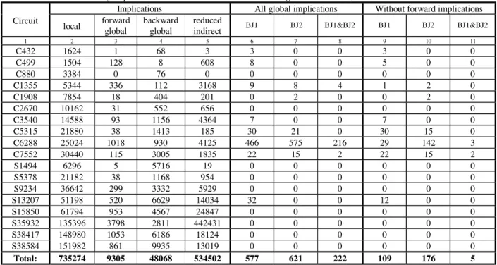
Table 2 shows the results of the backward justification. Columns 2-5 show the number of local implications, forward and backward global implications and the number of reduced indirect implications by removing all forward global implications. Columns 6-11 show the number of aborted backward justifications using heuristics BJ1, BJ2 and BJ1&BJ2 in two cases: (1) when all global implications were used; and (2) when all forward global implications were removed. Avoiding overspecification, we reduced significantly the number of aborted justifications 81.11%, 71.66% and 97.75%, respectively.
Table 3 shows the final results: columns (2-3), the average and maximum number of binary variables in CNF formula (size of problem), columns (4-5), the average and maximum depth of decision tree, columns (6-7), the average and maximum number of value assignments (excluding static learning), column (8-9), the average and maximum number of specified primary inputs, and columns (10-12), the number of test sessions that need less than 10, 100 and 1000 value assignments. The last column (13) presents test generation time in seconds. In some cases, the time for static learning was more than 50% of the test generation time (circuits S35932 and S38584) [4]. To decrease preprocessing time, we applied a Figure 5. Network example 5
P N M
K L
D
D D 1 0
0 1 A
G B =0
C = 1 D = 1 E F = 0
s-a-0
H
I J
restricted static learning when a huge dependency between signals was found (the average number of set variables by value assignment is greater than 100).
Since SPIRIT processes a single cone, the number of test sessions was usually bigger than the number of faults in the collapsed fault list. For example, the number of test sessions for circuit S15850 was 88% more than the number of the processed faults when the average ratio was 9.9% (see Table 1). On the other hand using a single cone processing, SPIRIT kept the size of problem as small as possible and increased effectiveness of 16-V search space reduction, SPOP and backward justification.
SPIRIT did not apply any techniques that required a special analysis or intensive computations such as dominators [18], X-path check [6], dependency-directed backtracking [15] or calculating transitive closure [3] which is equivalent to the first level recursive learning [4]. After static learning and 16-V search space reduction, the proposed TPG algorithm selected and set a variable in the CNF formula to a value according to the current objective, propagation or justification. Therefore, the number of value assignments assesses the efforts spent for satisfying the CNF formula. In this sense, the ratio between columns (6) and (4) and between (6) and (8) estimates the spare assignments and the number of assignments necessary to determine the value of one primary input. Except for the circuits C432 and C6288 the average number of specified primary inputs was larger than the average number of assignments which demonstrated the effectiveness of the presented backward justification procedure in respect to the PODEM approach. The effectiveness of the proposed justification procedure would be clarified more precisely if the assignments of the unsuccessful test sessions (no test patterns exist) were excluded when the average number of assignments was calculated. This correction changed most significantly this parameter for the circuit S15850 to 5.2, but this was not enough to change the relation between these two parameters. Also, the maximum number of assignments was usually smaller than the average number of variables in the CNF formula (size of problem) which demonstrated the efficiency of our TPG algorithm.
For this benchmark set, the total time was 172.33 seconds which made SPIRIT competitive to the best published ATPG systems ATOM [8] (371.6 seconds on a 200 MHz Pentium Pro PC), TEGUS [19] (477 seconds on a 200 MHz Pentium Pro PC) and TIP [20] (908 seconds on Digital Alpha 4100 5/533).
We believe that the advantages of SPIRIT will be more visible with more difficult benchmark circuits. For example, LookBack is the basic technique of ATOM since without LookBack, 999 faults in the circuits C5315, C6288 and S13207 will be aborted [8]. However, this technique is ineffective in respect to redundant faults. If
the processed benchmark circuits had many hard to prove redundant faults, then the LookBack technique could degrade the overall performance of ATOM. Also, SPIRIT is a single-phase TPG algorithm and a single-phase version of ATOM (1132 seconds on a 200 MHz Pentium Pro PC) is much slower than SPIRIT. On the other hand, the presented TPG algorithm gives an efficient solution for overspecification. Without special efforts, SPIRIT achieved comparable results for the maximum number of specified primary inputs as a problem oriented TPG algorithm presented in [9].
8. Conclusions
In this paper we presented an efficient TPG algorithm based on the Boolean Satisfiability method. We examined some not so popular approaches as a single cone processing, single path oriented propagation and backward justification, and proposed efficient techniques and heuristics for these approaches. To assess the effectiveness of SPOP and backward justification, we implemented them in SPIRIT [5] - ATPG system using a static order typical for the SAT-based TPG algorithms. As a result, a considerable impact on the efficiency and robustness has been achieved. Without fault simulator, SPIRIT was able to generate complete test sets and prove all redundant faults in the ISACAS’85 and ISCAS’89 benchmark circuits in a short amount of time. These results could be achieved even without dynamic learning but we kept this powerful technique to guarantee the robustness of our TPG algorithm for future applications as test generation for large combinational circuits and logic built-in self-test.
References:
[1] F.Brglez and H.Fujiwara, "A Neutral Netlist of 10 Combinational Benchmark Circuits and a Target Translator in Fortran," Proc. IEEE ISCAS, 1985, pp. 663-698.
[2] F.Brglez, D.Bryan and K.Kozminski,
"Combinational Profiles of Sequential Benchmark Circuits," Proc. IEEE ISCAS, 1989, pp.1929-1934. [3] S.Chakradhar, V.D.Agarval and S.Rothweiler, “A
Transitive Closure Algorithm for Test Generation,” IEEE Trans. on CAD, vol. 12, No.7, July 1993, pp.1015-1028.
[4] E.Gizdarski and H.Fujiwara, “A New Data Structure for Complete Implication Graph with Application for Static Learning”, technical report NAIST-IS- TR2000001, January 2000, pp.18. (http://isw3.aist- nara.ac.jp/IS/TechReport2/report/2000001.ps) [5] E.Gizdarski, "Test Pattern Generation using Boolean
Satisfiability," Automatica and Informatics, vol-32, No.2, 1998, pp. 33-40.
[6] P.Goel, “An Implicit Enumeration Algorithm to Generate Tests for Combinational Logic Circuits,” IEEE Trans. on Computers, vol. C-30, No.3, March 1981, pp.215-222.
[7] H.Fujiwara and T.Shimono, ”On Acceleration of Test Generation Algorithms,” IEEE Trans. on Computers, vol. C-32, No.12, Dec.1983, pp.1137- 1144.
[8] I.Hamzaoglu and J.H.Patel, “New Techniques for Deterministic Test Pattern Generation”, Journal of Electronic Testing: Theory and Applications, vol.-15, No.1/2, 1999, pp.63-73.
[9] S.Hellebrand, B.Reeb, S.Tarnick and H.J.Wunderlich, “Patter Generation for a Deterministic BIST Scheme,” Proc.IEEE/ACM ICCAD, 1995, pp.88-94.
[10] M.Henftling, H.Wittmann and K.Antreich, "A Single-Path-Oriented Fault-Effect Propagation in Digital Circuits Considering Multiple-Path Sensitization," Proc. IEEE/ACM ICCAD, 1995, pp.304-309.
[11] S.Kundu, L.M.Huisman, I.Nair, V.Iyengar and L.N.Ready “A Small Test Generation for Large Designs,” Proc. IEEE ITC, 1992, pp.30-40.
[12] W.Kunz and D.K.Pradhan, "Recursive Learning: A New Implication Technique for Efficient Solutions to CAD Problems–Test, Verification, and Optimization," IEEE Trans. on CAD, vol.13, No.9, Sept.1994, pp.1143-1158.
[13] T.Larrabee, "Test Pattern Generation Using Boolean Satisfiability," IEEE Trans. on CAD, vol.11, No.1, Jan.1992, pp.4-15.
[14] U.Mahlstedt, T.Gruning, C.Ozcan and W.Daehn,
“CONTEST: A Fast ATPG Tool for Very Large Combinational Circuits”, Proc. IEEE/ACM ICCAD, 1990, pp.222-225.
[15] J.Marques-Silva and K.A.Sakallah, "Dynamic Search Pruning Techniques in Path Sensitization," Proc. IEEE/ACM DAC, 1994, pp.705-711.
[16] P.Muth, "A Nine-Value Logic Model for Test Generation," IEEE Trans. on Computers, vol.C-25, No.6, June 1976, pp.630-636.
[17] J.Rajski and H.Cox, “A Method to Calculate Necessary Assigmnets in Algorithmic Test Generation”, Proc. IEEE ITC, 1990, pp.25-34. [18] M.Schulz, E.Trischler and T.Sarfert, "SOCRATES:
A High Efficient Automatic Test Pattern Generation System," IEEE Trans. on CAD, vol.7, No.1., Jan. 1988, pp.126-137.
[19] P.Stephan, R.K.Brayton and A.L.Sangiovanni- Vincentelli, “Combinational Test Generation using Satisfiability,” IEEE Trans. on CAD, vol.15, No.9, Sept.1996, pp.1167-1176.
[20] P.Tafertshofer and A.Ganz, "SAT Based ATPG Using Fast Justification and Propagation in the Implication Graph," Proc. IEEE/ACM ICCAD, 1999, pp.139-146.
[21] M.Teramoto, “A Method for Reducing the Search Space in Test Pattern Generation,” Proc. IEEE ITC, 1993, pp.429-435.
[22] J.A.Waicukauski, P.A.Shupe, D.J.Giramma and A.Martin, “ATPG for Ultra-Large Structural Designs,” Proc. IEEE ITC, 1990, pp.44-51.
Table 1: The number of sensitized propagation paths for successful/unsuccessful test sessions
Successful test sessions Unsuccessful test sessions #faults #test #test Circuit
paths=1 =2 =3 =4 =5 SSR paths=0 =1 =2 sessions patterns
C432 517 3 0 0 0 0 27 0 0 524 547 520
C499 750 0 0 0 0 0 156 0 0 758 906 750
C880 942 0 0 0 0 0 0 0 0 942 942 942
C1355 1566 0 0 0 0 0 156 0 0 1574 1722 1566
C1908 1870 0 0 0 0 0 177 0 0 1879 2047 1870
C2670 2627 3 0 0 0 220 90 9 0 2747 2949 2630
C3540 3291 0 0 0 0 0 649 0 0 3428 3940 3291
C5315 5287 4 0 0 0 84 177 9 8 5350 5569 5291
C6288 7707 3 0 0 0 0 380 0 0 7744 8090 7710
C7552 7400 12 4 2 1 86 1294 0 0 7550 8799 7419
S1494 1494 0 0 0 0 0 13 0 0 1506 1507 1494
S5378 4563 0 0 0 0 83 235 0 0 4603 4881 4563
S9234 6471 3 1 0 0 130 833 0 0 6927 7438 6475
S13207 9653 11 0 0 0 74 1020 16 0 9815 10774 9664
S15850 11336 0 0 0 0 765 9968 0 0 11725 22069 11336
S35932 35110 0 0 0 0 0 5376 0 0 39094 40486 35110
S38417 31015 0 0 0 0 36 1052 0 0 31180 32103 31015
S38584 34797 0 0 0 0 267 964 0 0 36303 36028 34797
Total: 166396 39 5 2 1 1745 22567 34 8 173649 190797 166443
Table 2: The number of implications and aborted test sessions using heuristics BJ1, BJ2 and BJ1&BJ2
Implications All global implications Without forward implications Circuit
local forward global
backward global
reduced
indirect BJ1 BJ2 BJ1&BJ2 BJ1 BJ2 BJ1&BJ2
1 2 3 4 5 6 7 8 9 10 11
C432 1624 1 68 3 3 0 0 3 0 0
C499 1504 128 8 608 8 0 0 5 0 0
C880 3384 0 76 0 0 0 0 0 0 0
C1355 5344 336 112 3168 9 8 4 1 2 0
C1908 7854 18 404 201 0 2 0 0 2 0
C2670 10162 31 552 656 0 0 0 0 0 0
C3540 14588 93 1156 4364 7 0 0 7 0 0
C5315 21880 38 1413 185 30 21 0 30 15 0
C6288 25024 1018 930 4125 466 575 216 29 142 3
C7552 30440 115 3005 1835 22 15 2 22 15 2
S1494 6296 5 5716 19 0 0 0 0 0 0
S5378 21182 38 1168 954 0 0 0 0 0 0
S9234 36642 299 3332 5929 0 0 0 0 0 0
S13207 51198 520 6629 14034 32 0 0 12 0 0
S15850 61794 953 4567 24847 0 0 0 0 0 0
S35932 135396 3798 2811 442431 0 0 0 0 0 0
S38417 148980 1053 6186 18124 0 0 0 0 0 0
S38584 151982 861 9935 13019 0 0 0 0 0 0
Total: 735274 9305 48068 534502 577 621 222 109 176 5
Table 3: Experimental results on the ISCAS’85 and full scan version of the ISCAS’89 benchmark circuits size of problem #levels of
decision tree
#value
assignments #specified inputs Distribution of test sessions according to #assignments Time Circuit
average max average max average max average max <10 <100 <1000 (sec.)
1 2 3 4 5 6 7 8 9 10 11 12 13
C432 124.8 204 15.5 35 17.1 186 12.1 26 136 408 3 0.14
C499 150.8 190 26.0 42 27.2 105 33.8 41 156 749 1 0.26
C880 102.2 187 8.6 19 9.6 20 9.7 23 379 563 0 0.17
C1355 381.5 462 27.3 35 28.6 94 35.9 41 156 1566 0 1.67
C1908 532.5 784 13.0 27 15.2 98 20.1 31 780 1267 0 2.08
C2670 306.9 1077 13.3 55 12.2 147 15.4 57 1277 1668 4 1.56
C3540 581.7 1832 9.1 37 10.2 119 13.4 30 2077 1858 5 5.07
C5315 272.0 1106 10.3 40 11.9 156 13.3 47 2349 3210 10 2.97
C6288 1327.2 3526 27.9 89 31.8 856 24.7 32 709 7323 58 49.17
C7552 547.2 1317 24.2 129 26.3 572 31.2 100 2243 6526 30 10.91
S1494 74.0 122 2.4 9 3.7 12 7.0 12 1502 5 0 0.80
S5378 134.8 571 3.8 46 4.9 50 7.9 36 4656 225 0 1.39
S9234 354.8 1238 5.1 27 6.1 28 11.7 43 5879 1559 0 3.88
S13207 188.9 2004 2.9 81 4.0 95 7.7 92 9949 825 0 7.04
S15850 625.4 1750 2.9 35 3.2 37 8.2 40 20713 1356 0 18.65
S35932 77.8 134 2.7 7 3.6 9 4.8 9 40486 0 0 27.41
S38417 197.1 641 10.0 78 11.1 79 13.1 85 21501 10602 0 21.66
S38584 93.2 1081 3.1 24 4.1 26 6.1 54 35108 920 0 17.50
Total: 285.1 3526 7.2 129 8.4 856 10.7 100 150056 40630 111 172.33