The synergy between sampling and advertising
Toshihiro Tsuchihashi ∗† September 2013
Abstract
Products are promoted in different ways. Specifically, if consumers face uncertainty about the product quality or characteristics, then sampling (to distribute free-samples) and advertising (to air television commercials) can effectively increase profits or revenues to firms. Actually, many firms simultaneously promote their products in the two ways, although single promotion may seem to serve for the purpose. This paper theoretically investigates the synergy between sampling and advertising, and finds that advertising in- creases profits not only directly through increase of the product price but also indirectly through increase of the optimal intensity for sampling.
1 Introduction
Firms promote their products in a variety of marketing activities in order to increase their sales or to expand market share. One of the most prominent promotion activities is advertis- ing. Firms often spend a vast amount of money on television commercials in which famous pop singers and actors emphasize attraction of the products. Sampling (distributing free-samples) is also important sales promotion, especially because consumers try free-samples and can be in- formed of attributes of products. Typically, free-samples of the products have been distributed on a street or through web sites,1 but consumers recently get free-samples through variety of channels as shown in Table 1.2
∗Faculty of Economics, Daito Bunka University: 1-9-1 Takashimadaira, Itabashi-ku, Tokyo, 175-8571, Japan; [email protected]
†I am very grateful to Tamotsu Kadoda and attendees at Lunch Seminar at Daito Bunka University and Microeconomics and Game Theory Workshop at Kyoto Institute of Economic Research (KIER) for helpful comments and suggestions. Any remaining errors are of course my own responsibility.
1Recently, consumers have been offered several kinds of free-samples (including cosmetics, cleaning products and snacks) on websites such as freesample.com in the US or Free sample hyakkaten in Japan.
2HANSOKU-KAIGI (Sales Promotion Meetings), September 2009, No. 137, p. 39.
Table 1: Consumer activities for getting free-samples
Activity %
Receive free-samples handed out on the streets 62.6 Apply for e-mail recruiting monitors via PCs 42.8 Go to sampling-spaces (where free-samples are distributed) 38.3 Apply for newspapers or magazines recruiting monitors 31.1 Apply for flyers or brochures recruiting monitors 28.8 Apply for direct mail recruiting monitors 22.3
Access to mobile phone sites 8.3
Apply for e-mail recruiting monitors via mobile phones 6.6
Consumers often face uncertainty about characteristics of products including quality, and then may hesitate to purchase the products. This is a typical lemon’s problem. However, these marketing activities can serve for information information revelation and avoid adverse selection problems, enhancing sales.
Advertising and sampling have been separately studied in the economics literature.
Advertising serves as a signal of product quality, because consumers correctly believe that firms spending much money provide high-quality products and remain the quality high. Nel- son (1970, 1974) is the first to argue a positive relationship between advertising and product quality, especially in experience goods market, and then the idea was formalized (Kihlstrom and Riordan, 1983; Milgrom and Roberts, 1986; Bagwell, 1992).3 Tellis and Fornell (1988) used the Profit Impact of Market Strategies database and empirically showed that product quality is positively correlated with advertising outlays. Nichols (1998) tested empirically the hypothesis that advertising functions as a signal of higher quality by using data of domestic and foreign automobile sales over the period 1985-1990, and he obtained results supporting the hypothesis.4
Sampling directly conveys product quality to consumers, since the consumers receive free-
3This type of advertising is referred to as informative advertising. The initial studies focus on a function of informative advertising to convey information about existence of sellers and their prices. These studies were likely to consider informative advertising as social waste of money. However, informative advertising recovered a positive position after Nelson (1970, 1974). See Bagwell’s (2003) survey on advertising. There also exist studies that an advertisement works as a signal of high quality if the marketing strategy is accompanied with a high price (Bagwell and Riordan, 1991; Linnemer, 2002).
4Some studies empirically critique the informative advertising (Horstmann and MacDonald, 1994, 2003).
samples and try them. Moraga-Gonzalez (2000) theoretically analyzes strategic sampling.5 His model engages in bilateral information asymmetry. The quality is a firm’s private information. On the other hand, consumers differently evaluate the expected quality based on some signal, but a firm cannot distinguish the consumers. A firm can reveal the quality to a certain rate of consumers by costly sampling. Moraga-Gonzalez found the positive correlation between the intensity of sampling and a price in equilibrium. In addition, he discussed conditions that the firm distributes free-samples in equilibrium: the consumer’s high valuation of the high-quality product; the high advertising cost; and the high likelihood of high-quality.6
If these promotions can inform consumers of the product quality, then firms should use one of them so that the firms can save money. Many firms, however, conduct several advertising campaigns by mixing television commercials and free-samples (promotion mix or marketing mix) in actual business transactions. This may imply a positive synergy between sampling and advertising; in other words, it may be valuable for the firms to employ both simultaneously. Narayanan, Desiraju and Chintagunta (2004, p. 90) pointed out: “[L]limited attentions has been devoted to the study of interactions among the elements of the marketing elements.” Some researches, however, empirically focused on interactions between marketing-mix elements, and discovered positive synergies.7 This paper theoretically explores the synergy between sampling and advertising, and gives theoretical foundation on the benefit of the promotion mix.
We introduce an adverse selection model similar to Moraga-Gonzalez (2000). A monopoly firm brings new products to a market. The firm’s ability is either high or low, and the firm with high ability provides the high-quality products while the firm with low ability produces the low-quality products. The ability is the firm’s private information. The firm can promote sales by advertising and/or sampling. The advertisements do not provide credible information about the quality, but the consumers may update their belief on the firm’s ability. The consumers actually know the quality if they receive free-samples. Finally, the firm chooses a price, and
5Moraga-Gonzalez refers to sampling as “informative advertising”.
6Strategic sampling has been also studied in the marketing literature. Heiman et al. (2001) constructed a dynamic duopoly model to determine the optimal effect of distributing free-samples. Bawa and Shoemaker (2004) analyzed the impact of strategic sampling on sales theoretically and found evidence to support the theory.
7The examples include, advertising and non-price promotions (Mela, Gupta, and Lehmann, 1997), advertising and sales force (Gatignon amd Jamssems, 1987), and sales force and samples (Parsons and Vanden Abeele, 1981). See Table 1 in Narayanan, Desiraju and Chintagunta (2004, p. 91).
the consumers decide whether to buy the products or not.
We find that a firm does not employ sampling solely, implying that there exists strategic complementarity between advertising and sampling. There exist three types of equilibria: (i) a no-promotion equilibrium where neither type of firms employs a promotion method, (ii) an advertising equilibrium where both types of firms employ advertising but sampling, and (iii) a promotion-mix equilibrium where both types of firms employ advertising and the high-type firm employs sampling in addition to advertising. We identify and characterize these equilibria. This paper is organized in the following way. Section 2 describes the model where a single firm can employ advertising in the first stage and sampling together in the second stage. Section 3 considers a separating equilibrium and shows that a separating equilibrium does not exist. Section 4 derives and characterizes a pooling equilibrium. Section 5 concludes, and the Appendix includes all the proofs.
2 The Model
We model a situation where a single firm is allowed to employ both advertising and sampling together. The single firm aims to bring new products to a market in which there are identical consumers whose mass is normalized to one and each of the consumers demands at most one unit of products. The firm’s ability to produce the products and to promote sales is either high (h) or low (ℓ). The ability is the firm’s private information, and the consumers initially believe that the firm’s ability is high with probability β ∈ (0, 1), which is exogenously given and is common knowledge.8 We refer to the firm with high (low) ability as an h-type (ℓ-type) firm. The h-type firm certainly produces the high-quality product whose value is qh = q > 0 to the consumers, while the ℓ-type firm certainly produces the low-quality product whose value is qℓ= 0 to the consumers. We assume that the production cost is zero.9 After producing the products, the firm can promote sales in two ways: advertising and sampling. The promotion is the firm’s strategic information revelation.
8The firm is involved in adverse selection problems as in Akerlof (1970).
9In this model, the firm is not involved in moral hazard problems, i.e., the firm cannot strategically choose the type, but instead the type is exogenously given. Therefore, the production cost does not play an important role. Even though we introduced a positive production cost for the h-type firm as in Moraga-Gonzalez (2000), the results would not essentially change.
Table 2: Timing of the Model Time Event
0 Firm privately learns its type: h (high) or ℓ (low)
1 Advertising: Firm chooses a rate of consumers watching an advertisement γ Sampling: Firm chooses a rate of consumers receiving free-samples λ
2 Pricing: Firm announces a price p
Purchase: Consumers decide whether to buy or not
Advertising. If the firm advertises its products with cost c > 0, then the certain rate of consumers watch the advertisement, e.g., television commercials. Note that the advertisement does not contain credible information about the firm’s type. We assume the rate of consumers watching an advertisement is a binary choice. Denote by γi the rate chosen by the i-type firm. We assume that γh∈ {0, ¯γ} and γℓ∈ {0, γ}, and naturally ¯γ ∈ (0, 1) and γ ∈ (0, 1).
Sampling. If the firm distributes free-samples of the new products, then the certain rate of the consumers receive and try the free-samples. Unlike the advertisement, the free-sample reveals the actual product quality and thus the firm’s type to the receiver. Note that the ℓ- type firm never chooses a positive rate because the ℓ-type firm does not want to reveal its type. Therefore, we assume that only the h-type firm can distribute the free-samples.10 We assume that the firm can directly choose the rate of consumers who receive the free-samples. Denote by λ ∈ {0, ¯λ} the rate chosen by the h-type firm. Choosing ¯λ bears cost k > 0 to the h-type firm. We assume that ¯λq ≥ k, implying that, the h-type firm earns a non-negative profit when only consumers receiving free-samples purchase products from the h-type firm for a price equal to the value of the high-quality product.
Pricing. Finally, the firm announces a price p, consumers then buy the product if the price is at or below their expected reservation values. Note that the price is a take-it-or-leave-it offer. The timing is shown in Table 2.
10This setting is the same as Moraga-Gonzalez (2000). Even though we allow the ℓ-type firm to distribute the free-samples, the ℓ-type firm would never employ sampling in any equilibrium.
We adopt Perfect Bayesian equilibrium (PBE) as a solution concept. Consumers update their belief based on price p and form an identical belief unless they receive the free-samples. However, the expected value for consumers may differ depending on whether they watch the advertisement and/or whether they receive the free-sample. We classify consumers into three types: (i) Sample Receiver : We refer to a consumer who receives a free-sample as Sample Receiver (hereafter, SR). Since SR can certainly understand the product quality and the firm’s type as well, SR assigns probability one on the correct type, i.e., the h type firm for sure, for any prices. Therefore, SR is willing to pay qh for the (high-quality) product. (ii) Ad Watcher : We refer to a consumer who does not receive a free-sample but watches an advertisement as Ad Watcher (hereafter AW). AW updates a belief after observing price p, and we denote the belief by ¯βe, that AW assigns probability ¯βe on the h-type firm. Since AW believes that the i-type firm chooses a rate of advertising γei and the h-type firm chooses a rate of sampling λe, Bayes’ rule gives the updated belief
β¯e= βγeh(1 − λe) βγeh(1 − λe) + (1 − β)γeℓ
. (1)
Consequently, AW is willing to pay for the product at
¯
qe= ¯βeqh+ (1 − ¯βe)qℓ = βγeh(1 − λe)q βγeh(1 − λe) + (1 − β)γeℓ
. (2)
(iii)Uninformed Consumer : We refer to a consumer who neither receives a free-samples nor watches an advertisement as Uninformed Consumer (hereafter UC). UC updates a belief after observing price p, and we denote the belief by βe. Bayes’ rule gives
βe= β(1 − γeh)
β(1 − γeh) + (1 − β)(1 − γeℓ). (3) Consequently, UC is willing to pay for the product at
qe= βeqh+ (1 − βe)qℓ = β(1 − γeh)(1 − λe)q
β(1 − γeh)(1 − λe) + (1 − β)(1 − γeℓ). (4) As usual, γe = (γeh, γeℓ) should be consistent with (γh, γℓ) on an equilibrium path. We assume that the consumers assign probability one to the ℓ-firm off the equilibrium path, i.e. β¯e = βe = 0, independent of γe and λe, unless they receive the free-samples. The belief is the most pessimistic, supporting the largest set of equiibria. Note that advertising may
create difference of the expected reservation values among the consumers. Note that by simple calculation, AW values the expected quality more than UC if and only if the h-type firm advertises more than the ℓ-type firm, that is, ¯qe> qe ⇔ γh > γℓ.11
We restrict our attention to a pure strategy as in Moraga-Gonzalez (2000). The equilibrium profile is represented by a triplet (p, γ, λ) where p = (ph, pℓ) and γ = (γh, γℓ). We distinguish a separating equilibrium and a pooling equilibrium based on a price proposed by the firm.
3 Separating equilibrium
We begin our discussion by showing that any equilibria should be a pooling equilibrium. Since different types of firms offer different prices in a separating equilibrium, an equilibrium price certainly conveys the product quality to all consumers. Therefore, costly promotion methods are redundant for both types of firms in a separating equilibrium. Without promotion, both types of firms have to offer the same price. To see this, suppose contrarily that ph ̸= pℓ in equilibrium. On observing ph, consumers believe that the quality is certainly high and thus they are willing to pay at qh. Therefore, the price phattracts whole demand if ph≤ qh, and zero demand if ph> qh, because all consumers are UC. Similarly, all consumers buy the product for price pℓ≤ qℓ while no consumers buys the product for pℓ > qℓ. Consequently, the h-type firm can profitably deviate to choose pℓ if pℓ > ph, while the ℓ-type firm can profitably deviate to choose ph if ph > pℓ. This argument leads to the following lemma.
Lemma 1. (Moraga-Gonzalez, 2000; Proposition 1) A separating equilibrium does not exist.
The following assumptions underline this lemma. First, the firm can understand neither who watches an advertisement nor who receives a free-sample, and the firm thus cannot offer different prices to AW, UC, and SR. If the firm can distinguish consumers, then for example the following separating equilibrium might exist: the h-type firm employs sampling and offer
11Moraga-Gonzalez (2000) constructed a model where some consumers observe an informative signal about the firm’s actual type before a firm decides to distribute free-samples. The signal is not the firm’s strategic choice, but instead a random variable. This is an important difference between our model and the Moraga-Gonzalez’s. A role of the signal in Moraga-Gonzalez (2000) is also to create difference of the expected reservation values among the consumers.
Table 3: Profiles of promotion (γh, γℓ, λ) Advertising & sampling (promotion-mix) (¯γ, γ, ¯λ) (¯γ, 0, ¯λ)
Advertising & sampling (separately) (0, γ, ¯λ)
Advertising (¯γ, γ, 0) (¯γ, 0, 0) (0, γ, 0)
Sampling (0, 0, ¯λ)
No promotion (0, 0, 0)
a high price for SR and a low price for the other consumers, and the ℓ-type firm offer the low price. Second, all consumer are ex ante identical. Therefore, without promotion, either all consumers buy the products and a firm obtains whole demand, or no consumer buys for any price and a firm obtains zero demand.
4 Pooling equilibrium
If we fix a price, then potentially there exist 23 = 8 profiles of (γh, γℓ, λ) as shown in Table 3. However, as the following lemmas show, equilibrium candidates are restricted to (¯γ, γ, ¯λ), (¯γ, γ, 0), and (0, 0, 0). The first profile represents promotion-mix in which the h-type firm employs both methods of promotion, while the last profile represents no-promotion in which no promotion method is employed in equilibrium.
Lemma 2. If ¯γ ≤ γ, no promotion is employed in any equilibrium, i.e. (γh, γℓ, λ) = (0, 0, 0).
¯
γ < γ gives that the ℓ-type firm advertises more than the h-type firm, implying that AW is less likely to pay for the product than UC. In other words, an advertisement conveys “bad” information to consumers in this case. Interestingly, Lemma 2 gives that the h-type firm does not employ sampling whenever advertising has no advantage. The intuition behind this is, the h-type firm cannot raise a price even if the h-type firm can reveal its type by sampling, because the h-type firm cannot distinguish consumers. In what follows, we consider a case of ¯γ > γ.
Lemma 3. Suppose ¯γ > γ. We obtain that (i) (γh, γℓ, λ) such that γℓ > γh ≥ 0 never con- structs an equilibrium for any λ, (ii) (γh, 0, λ) such that γh > 0 never constructs an equilibrium
for any λ, and (iii) (0, 0, ¯λ) never constructs an equilibrium.
The intuition behind this lemma is as follows. First, (i) gives that the ℓ-type firm does not advertise products more than the h-type firm, and excludes profiles of (γh, γℓ, λ) = (0, γ, 0) and (0, γ, ¯λ) from an equilibrium. To see this, suppose contrarily that the ℓ-type firm advertised products more than the h-type firm. In this case, an advertisement would work as a “bad signal”, and thus AW would value the products less then UC. Consequently, both types of firms could profitably choose zero advertisement. This result is intuitive. Second, (ii) gives that the h-type firm does not solely advertise products, and excludes (γh, γℓ, λ) = (¯γ, 0, 0) and (¯γ, 0, ¯λ). Solely advertising by the h-type firm certainly informs consumers of high-quality, but the firm could not charge a high price because UC would not buy products for the high price. Consequently, advertising would not raise the h-type firm’s profit and the h-type firm does not solely advertise products. Third, (iii) gives that an equilibrium engaging in sampling solely does not exist, and excludes (γh, γℓ, λ) = (0, 0, ¯λ).
We seek a pooling equilibrium by backward induction. In the second stage, given (γ, λ), the firm chooses price p. Consumers form a belief βe and value the expected quality at qegiven by (2) and (4). Denote a demand function of the i-type firm by Di(p; γi, γe; λ, λe) for price p when the i-type firm chooses γi, the h-type firm chooses λ, and the consumers infer (γe, λe). Note that in equilibrium γi = γe for i = h and ℓ and λ = λe hold. Since γh ≥ γℓ, the demand function is given as follow:
Firstly, we consider the demand function of the ℓ-type firm. Since the ℓ-type firm never distributes free-samples, consumers are AW and UC. UC will buy the products for price p ≤ qe, and AW will buy the products for price p ≤ ¯qe. No consumer will buy the products for price p > ¯qe. Therefore, the ℓ-type firm’s demand function is given by:
Dℓ(p; γℓ, γe; 0, λe) =
1 if p ≤ qe
γℓ if qe< p ≤ ¯qe
0 if p > ¯qe.
(5)
Similarly, we next consider the demand function of the h-type firm. If the h-type firm chooses a positive rate of consumers to be SR, then SR correctly knows the product quality, and will
buy the product for price p ≤ q. On the other hand, UC will buy products for price p ≤ qe, and AW will buy products for price p ≤ ¯qe. No consumer will buy products for price p > ¯qe. Therefore, the h-type firm’s demand function is given by:
Dh(p; γh, γe; λ, λe) =
1 if p ≤ qe
γh+ λh(1 − γh) if qe < p ≤ ¯qe
λ if ¯qe < p ≤ q
0 if p > q.
(6)
4.1 No-promotion equilibrium
We derive an equilibrium price in a no-promotion equilibrium where neither type of firms employs any promotion methods, i.e., (γh, γℓ, λ) = (0, 0, 0). Note that γh = γℓ = 0 leads to
¯
qe = qe = βqh+ (1 − β)qℓ = βq. In equilibrium, therefore, both types of firms should choose price p∗ ≤ βq which yields whole demand (i.e., UC and AW) and the profit Π∗h = Π∗ℓ = p∗ to the firm. This is because no consumer buys products for any price p∗ > βq.
Proposition 1. (No-promotion equilibrium) The profile (p∗, (γh∗, γℓ∗), λ∗) = (p∗, (0, 0), 0) constructs a no-promotion equilibrium where p∗ ∈ [¯λq − k, βq]. A no-promotion equilibrium exists if and only if k ≥ (¯λ − β)q.
Since the no-promotion equilibrium is a pooling equilibrium, the consumers do not update the initial belief on the equilibrium path. Therefore, the equilibrium price cannot exceed the expected value under the initial belief. The lower bound of the equilibrium price ensures that neither type of the firm could profitably deviate to low prices and middle prices accompanied by sampling. The existence condition implies (i) the high cost of sampling, (ii) the high likelihood of high quality, and (iii) the low value of the high-quality product. These implications are consistent with the condition of existence of the no-advertising equilibrium in Moraga-Gonzalez (2000). Intuition behind the existence condition is as follows. First, the higher cost of sampling makes the high type firm reluctant to distribute free-samples. Otherwise, the high type firm could benefit from sampling and then choosing higher prices. Second, if the consumers initially believe that the firm’s type is high with a sufficiently high probability, then the firm need not promote sales by employing costly promotion methods. Conversely, the lower initial probability
of the high type firm enhances the value of the promotion methods; thus, the no-promotion equilibrium is less likely to realize. Third, if the values of the high-quality is not high, the firm would not benefit from appealing the high-quality, because the consumers’ willingness to pay does not increase very much even if the consumers actually knows that the product quality is high.
4.2 Advertising equilibrium
We derive an equilibrium price in an advertising equilibrium where both types of firms choose a positive rate of advertising but sampling does not appear, i.e., (γh, γℓ, λ) = (¯γ, γ, 0). In equilibrium, therefore, an equilibrium price p∗ should lie between (qe, ¯qe] for which AW buys the product but UC does not. This is because (i) all consumers (i.e., UC and AW) buy the product for price p∗ ≤ qe and thus costly advertising is redundant, and (ii) no consumer buys the product for price p∗ > ¯qe. The price p∗ yields profit Π∗h = ¯γp∗− c to the h-type firm and profit Π∗ℓ = γp∗− c to the ℓ-type firm, respectively. By substituting γeh = ¯γ, γeℓ = γ and, λe= 0 into (2) and (4), we obtain
qe= β(1 − ¯γ)q
β(1 − ¯γ) + (1 − β)(1 − γ),
¯
qe= β¯γq β¯γ + (1 − β)γ.
Proposition 2. (Advertising equilibrium) The profile (p∗, (γh∗, γℓ∗), λ∗) = (p∗, (¯γ, γ), 0) constructs an advertising equilibrium where the equilibrium price p∗lies between (qe, ¯qe] where
qe= β(1 − ¯γ)q
β(1 − ¯γ) + (1 − β)(1 − γ), (7)
¯
qe= β¯γq
β¯γ + (1 − β)γ (8)
and satisfies
p∗ ≥ max{c γ,
λq − k + c¯
¯ γ
}≡ X (9)
p∗ ≤ ¯ k
λ(1 − ¯γ). (10)
Since the ℓ-type firm cannot earn a positive profit by any deviations, it is enough for the ℓ- type firm that the equilibrium price covers the cost of advertising; thus, this gives a lower-bound of an equilibrium price.
On the other hand, the h-type firm has two potentially profitable deviations. The first one is to employ sampling in addition to advertising. The h-type firm would maintain a price with this deviation, because the h-type firm intends to sell products to SR and AW. This deviation brings the h-type firm a trade-off between the benefit from additional sales to SR and the cost of sampling. The additional sales monotonically increase in the remaining equilibrium price; thus, the h-type firm could benefit from this deviation if the price is sufficiently high. Consequently, this gives an upper-bound of an equilibrium price. The second one is to switch a promotion behavior from advertising to sampling. Since the h-type firm would face UC and SR with this deviation, the h-type firm would charge a high price aimed at selling products to SR. The second deviation shows a trade-off between the benefit from increase of a price and the loss from decrease of demand. A sufficiently high equilibrium price reduces the benefit; thus, this gives a lower-bound of an equilibrium price.
The next proposition gives the existence condition of the advertising equilibrium.
Proposition 3. (Existence of advertising equilibrium) An advertising equilibrium ex- ists if and only if either (i) (A1), (A2), and (A3) hold, or (ii) (A1), (A2), (A4), and (A5) hold, where
γ 1 − ¯γ ≥
λc¯
k , (A1)
¯ γ 1 − ¯γ ≥
λ(¯¯ λq − k + c)
k , (A2)
q < k (1 − ¯γ)2λ¯
(
− (¯γ − γ) + 1 − γ β
)
, (A3)
q ≥ c
¯ γ
(¯γ − γ
¯
γ +
γ
¯ γ ·
1 β
)
, (A4)
[(¯γ2− (¯γ − γ)¯λ)β − γ¯λ]q + (k − c)[(¯γ − γ)β + γ] ≥ 0. (A5)
Proposition 3 shows that an advertising equilibrium exists if (i) the cost of advertising is low, (ii) the cost of sampling is high, (iii) a ratio of SR (or efficiency of sampling) is low, and (iv) a
ratio of AW (or efficiency of advertising) is high. Intuitions underlying Proposition 3 are simple. These are intuitive. The low cost of advertising and the high efficiency of advertising together enhance the firm’s incentive to employ costly advertising, while the high cost of sampling and the low efficiency of sampling together soften the firm’s incentive to employ costly sampling.
(A3), (A4), and (A5) give hyperbolas in a (q, β)-plane. (q, β) with higher q and higher β are likely to satisfy (A4) and (A5), but (A3) gives the upper-bound of q which is decreasing in β. Note that, for (A5), (i) if a co-efficient of q is positive and k ≥ c, or (ii) if the co-efficient is negative and k ≤ c, then (A5) is never satisfied since (i) or (ii) implies q ≤ 0.
4.3 Promotion-mix equilibrium
We derive an equilibrium price in a promotion-mix equilibrium where both types of firms choose a positive rate of advertising and the h-type firm chooses a positive rate of sampling, i.e., (γh, γℓ, λ) = (¯γ, γ, ¯λ). In equilibrium, therefore, an equilibrium price p∗ should lie between (qe, ¯qe] for which AW and SR buy the product but UC does not. As in the advertising equilib- rium, this is because (i) all consumers (i.e., UC and AW) buy the product for price p∗≤ qeand thus costly advertising is redundant, and (ii) no consumer buys the product for price p∗> ¯qe. The price p∗yields profit Π∗h = (¯γ + ¯λ(1− ¯γ))p∗−c−k to the h-type firm and profit Π∗ℓ = γp∗−c to the ℓ-type firm, respectively. By substituting γeh = ¯γ, γeℓ= γ, and λe= ¯λ into (2) and (4), we obtain
qe= β(1 − ¯γ)(1 − ¯λ)q
β(1 − ¯γ)(1 − ¯λ) + (1 − β)(1 − γ),
¯
qe= β¯γ(1 − ¯λ)q β¯γ(1 − ¯λ) + (1 − β)γ.
Proposition 4. (Promotion-mix equilibrium) The profile (p∗, (γh∗, γℓ∗), λ∗) = (p∗, (¯γ, γ), ¯λ) constructs a promotion-mix equilibrium where the equilibrium price p∗ lies between (qe, ¯qe] where
qe = β(1 − ¯γ)(1 − ¯λ)q
β(1 − ¯γ)(1 − ¯λ) + (1 − β)(1 − γ), (11)
¯
qe= β¯γ(1 − ¯λ)q
β¯γ(1 − ¯λ) + (1 − β)γ, (12)
and satisfies
p∗ ≥ max{c γ,
¯λq + c
¯
γ + (1 − ¯γ)¯λ, k (1 − ¯γ)¯λ
}≡ Y. (13)
As in the advertising equilibrium, no profitable deviation for the ℓ-type firm induces a lower-bound of an equilibrium price. The h-type firm has two potentially profitable devia- tions: advertising solely with the remaining a price, and sampling solely with a high price. As previously, the deviation to sampling solely with a high price induces a lower-bound of an equi- librium price. The deviation to advertising solely with the remaining price shows a trade-off between the benefit from saving the cost of sampling and the loss from decrease of sales to SR. Since the higher remaining price yields the larger loss to the h-type firm and loses an incentive to this deviation, this gives a lower-bound of an equilibrium price.
The next proposition gives the existence condition of the promotion-mix equilibrium.
Proposition 5. (Existence of promotion-mix equilibrium) A promotion-mix equilib- rium exists if and only if (P1), (A2), (P3), and (A4) hold, where
q ≥ c
¯
γ(1 − ¯λ)
[γ(1 − ¯¯ λ) − γ
γ +
1 β
], (P1)
q ≥ γk
¯
γ(1 − ¯γ)(1 − ¯λ)¯λ
[γ(1 − ¯¯ λ) − γ
γ +
1 β ]
, (P2)
[((¯γ(1 − ¯λ))2+ γ¯λ)β − γ¯λ]q ≥ [(¯γ(1 − ¯λ) − γ)β + γ]c, (P3) β > γ¯λ
[¯γ(1 − ¯λ)]2+ γ¯λ ≡ ¯β. (P4)
For (P3) to hold, a co-efficient of q in (P3) must be positive, which is ensured by (A4). Therefore, there exists a lower-bound of β, independent of q, for existence of a promotion-mix equilibrium. (P1), (P2), and (P3) give hyperbolas in a (q, β)-plane, and (q, β) with higher q and higher β are likely to satisfy these conditions.
5 Analysis
It may be interesting to compare equilibrium prices and equilibrium profits among a no- promotion equilibrium (hereafter, NPE), and advertising equilibrium (hereafter, ADE), and
a promotion-mix equilibrium (hereafter, PME). As shown in the above discussion, however, there are multiple equilibria in each type of equilibria, i.e., NPE, ADE, and PME. Therefore, in this section, we focus on the maximum equilibrium price in each type of equilibria.12 Note that given an equilibrium price, the firm eqrns a higher profit in an NPE than in ADE and PME, because all consumers buy products for the equilibrium price in an NPE and the firm pays positive costs for promotion in ADE and PME. Since generally comparing equilibria is very complicated, we consider some numerical examples.
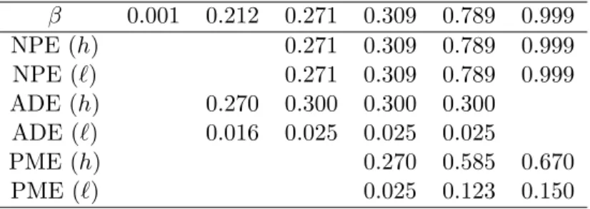
First, suppose that q = 1, c = 0.10, ¯γ = 0.80, γ = 0.25, k = 0.03, and ¯λ = 0.30. In this case, the cost of advertising is higher than the cost of sampling (c = 0310 > k = 0.03), and the unit cost of advertising is higher for the h-type firm than that of sampling (c/¯γ = 0.125 > k/¯λ = 0.100). Under these parameters, an NPE exists for β ∈ [0.271, 1), an ADE exists for β ∈ [0.212, 0.789], and a PME exists for β ∈ [0.309, 1); thus, NPE, ADE, and PME simultaneously exist for β ∈ [0.309, 0.789]. Table 4 shows the maximum equilibrium prices, and the corresponding equilibrium profits are shown in Table 5. β = 0.309 gives the maximum equilibrium prices: p∗ = 0.309 in an NPE, p∗ = 0.500 in an ADE, and p∗ = 0.500 in a PME; and the equilibrium profits (Π∗h, Π∗ℓ) = (0.309, 0.309) in an NPE, (Π∗h, Π∗ℓ) = (0.300, 0.025) in an ADE, and (Π∗h, Π∗ℓ) = (0.270, 0.025) in a PME. On the other hand, β = 0.789 gives the maximum equilibrium prices: p∗ = 0.789 in an NPE, p∗ = 0.500 in an ADE, and p∗ = 0.893 in a PME; and the equilibrium profits (Π∗h, Π∗ℓ) = (0.789, 0.789) in an NPE, (Π∗h, Π∗ℓ) = (0.300, 0.025) in an ADE, and (Π∗h, Π∗ℓ) = (0.585, 0.123) in a PME. In all of NPE, ADE, and PME, both the maximum equilibrium prices and the corresponding equilibrium profits are non-decreasing in β. The h-type firm can earn a higher profit in an ADE than in an NPE at β = 0.271 (a low probability of a high-type firm), while both types of firms can earn a higher profit in an NPE than in ADE and PME at a higher β. Intuitively, promotion is too costly to make a profit even though it could push up a price. In ADE and PME, the h-type firm obtains the higher profits than the ℓ-type firm, because the h-type firm can sell products to more consumers than the ℓ-type firm.
12If we assume that consumers form a monotone-belief in which they assign a higher probability on an h-type for a higher price, then an equilibrium price is uniquely determined as the upper-bound of equilibrium prices in each type of equilibria. To see this, let [p, ¯p] be a set of equilibrium prices under the most pessimistic belief in the above discussion. The monotone belief implies that, if a consumer buys a product for price p1∈[p, ¯p], then the consumer will buy a product for p2∈[p, ¯p], p2> p1. Therefore, the firm optimally chooses ¯p.
Table 4: The maximum equilibrium prices β 0.001 0.212 0.271 0.309 0.789 0.999
NPE 0.271 0.309 0.789 0.999
ADE 0.463 0.500 0.500 0.500
PME 0.500 0.893 1.000
Table 5: Equilibrium profits given the maximum equilibrium prices β 0.001 0.212 0.271 0.309 0.789 0.999
NPE (h) 0.271 0.309 0.789 0.999
NPE (ℓ) 0.271 0.309 0.789 0.999
ADE (h) 0.270 0.300 0.300 0.300 ADE (ℓ) 0.016 0.025 0.025 0.025
PME (h) 0.270 0.585 0.670
PME (ℓ) 0.025 0.123 0.150
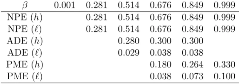
Second, suppose that q = 1, c = 0.15, ¯γ = 0.6, γ = 0.25, k = 0.12, and ¯λ = 0.4. In this case, the cost of advertising is higher than the cost of sampling (c = 0.15 > k = 0.12), but the unit cost of advertising is lower for the h-type firm than that of sampling (c/¯γ = 0.25 < k/¯λ = 0.30). Under these parameters, an NPE exists for β ∈ [0.281, 1), an ADE exists for β ∈ [0.514, 0.849], and a PME exists for β ∈ [0.676, 1); thus, NPE, ADE, and PME simultaneously exist for β ∈ [0.676, 0.849]. Table 6 shows the maximum equilibrium prices, and the corresponding equilibrium profits are shown in Table 7. β = 0.676 gives the maximum equilibrium prices: p∗ = 0.676 in an NPE, p∗ = 0.750 in an ADE, and p∗ = 0.750 in a PME; and the equilibrium profits (Π∗h, Π∗ℓ) = (0.676, 0.676) in an NPE, (Π∗h, Π∗ℓ) = (0.300, 0.038) in an ADE, and (Π∗h, Π∗ℓ) = (0.180, 0.038) in a PME. On the other hand, β = 0.849 gives the maximum equilibrium prices: p∗ = 0.849 in an NPE, p∗ = 0.750 in an ADE, and p∗ = 0.890 in a PME; and the equilibrium profits (Π∗h, Π∗ℓ) = (0.676, 0.676) in an NPE, (Π∗h, Π∗ℓ) = (0.300, 0.038) in an ADE, and (Π∗h, Π∗ℓ) = (0.264, 0.073) in a PME. Both the equilibrium price and profits monotonically increase in β in NPE and PME, and remain constant in PME. Unfortunately, promotion strategies increase not only demand but also the cost.
Third, suppose that q = 1, c = 0.05, ¯γ = 0.40, γ = 0.25, k = 0.17, and ¯λ = 0.40. In
Table 6: The maximum equilibrium prices β 0.001 0.281 0.514 0.676 0.849 0.999 NPE 0.281 0.514 0.676 0.849 0.999
ADE 0.717 0.750 0.750
PME 0.750 0.890 0.999
Table 7: Equilibrium profits given the maximum equilibrium prices β 0.001 0.281 0.514 0.676 0.849 0.999 NPE (h) 0.281 0.514 0.676 0.849 0.999 NPE (ℓ) 0.281 0.514 0.676 0.849 0.999
ADE (h) 0.280 0.300 0.300
ADE (ℓ) 0.029 0.038 0.038
PME (h) 0.180 0.264 0.330
PME (ℓ) 0.038 0.073 0.100
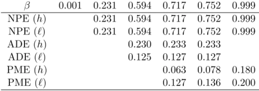
this case, the cost of advertising is lower than the cost of sampling (c = 0.05 < k = 0.17), and the unit cost of advertising is lower for the h-type firm than that of sampling (c/¯γ = 0.125 < k/¯λ = 0.425). Under these parameters, an NPE exists for β ∈ [0.231, 1), an ADE exists for β ∈ [0.594, 0.752], and a PME exists for β ∈ [0.717, 1); thus, NPE, ADE, and PME simultaneously exist for β ∈ [0.717, 0.752]. Table 8 shows the maximum equilibrium prices, and the corresponding equilibrium profits are shown in Table 9. β = 0.717 gives the maximum equilibrium prices: p∗ = 0.717 in an NPE, p∗ = 0.708 in an ADE, and p∗ = 0.709 in a PME; and the equilibrium profits (Π∗h, Π∗ℓ) = (0.717, 0.717) in an NPE, (Π∗h, Π∗ℓ) = (0.233, 0.127) in an ADE, and (Π∗h, Π∗ℓ) = (0.063, 0.127) in a PME. On the other hand, β = 0.752 gives the maximum equilibrium prices: p∗ = 0.752 in an NPE, p∗ = 0.708 in an ADE, and p∗ = 0.744 in a PME; and the equilibrium profits (Π∗h, Π∗ℓ) = (0.752, 0.752) in an NPE, (Π∗h, Π∗ℓ) = (0.233, 0.127) in an ADE, and (Π∗h, Π∗ℓ) = (0.078, 0.136) in a PME. As in the previous case, in all of NPE, ADE, and PME, both the maximum prices and the corresponding equilibrium profits are non-decreasing in β. The h-type firm can earn the highest profit in an NPE, the second-highest one in an ADE, and the lowest one in a PME. In this case also, promotion is too costly to make a profit. Unlike the previous cases, the equilibrium profits to the h-type firm is
Table 8: The maximum equilibrium prices β 0.001 0.231 0.594 0.717 0.752 0.999 NPE 0.231 0.594 0.717 0.752 0.999
ADE 0.701 0.708 0.708
PME 0.709 0.744 0.999
Table 9: Equilibrium profits given the maximum equilibrium prices β 0.001 0.231 0.594 0.717 0.752 0.999 NPE (h) 0.231 0.594 0.717 0.752 0.999 NPE (ℓ) 0.231 0.594 0.717 0.752 0.999
ADE (h) 0.230 0.233 0.233
ADE (ℓ) 0.125 0.127 0.127
PME (h) 0.063 0.078 0.180
PME (ℓ) 0.127 0.136 0.200
lower than that to the ℓ-type firm, because the cost of sampling is expensive in this case. Therefore, we obtain the following observations.
Observation 1. (Equilibrium price) The maximum equilibrium price is non-decreasing in β in an ADE, and is increasing in β in both NPE and PME. What equilibrium induces the highest maximum equilibrium price is not determined; ti other words, neither advertising nor sampling can fail in rising prices.
Observation 2. (Equilibrium profit) The equilibrium profits corresponding to the max- imum equilibrium price is non-decreasing in β in an ADE, and is increasing in β in both NPE and PME. Both types of the firms obtain the highest profit in an NPE; in other words, promotion causes a decline in a profit even though it raises a price.
Observation 1 and Observation 2 suggests that promotion strategies generate a negative result rather than a beneficial one for a firm even though promotion serves for a signal of high-quality, diminishes information asymmetry, and improves efficiency of trading, because
the costs for promotion is too expensive. These theoretical predictions seem consistent with empirical evidences.*** Assmus, et al. (1984) discuss that it is difficult to identify the impact of advertising on sales in both short-term and long-term advertising response.
6 Concluding remarks
Consumers are not always sure the product quality prior to purchase. In this case, firms usually promote their products in forms of sampling and advertising to convey information about the quality to the consumers. Since both promotion methods seem to work similarly, employing just one method rather than both of them seems to be enough for firms to convey information. However, we often observe that these two promotions are simultaneously employed by a single firm, which may imply a positive synergy of promotion mix.
We conducted a theoretical model to investigate the positive synergy. In our model, a monopoly firm provides new products to market, and before setting a price, it can promote its products by sampling and advertising. The firm chooses intensity of sampling and advertising volume, respectively. Consumers know the quality by receiving the free samples, while they infer the quality by watching TV commercials.
We find strategic complementarity between advertising and sampling. Thus, there exists two types of equilibria where (i) neither sampling nor advertising occurs, and (ii) both sampling and advertising together occur. The result is consistent with the observations in marketing literature that prior advertising can raise the the proportion of consumers who use the free samples. Also, some experiment studies confirm the positive effect of advertising on sampling. Furthermore, this kind of promotion-mix is observed in actual business transactions; thus, the result can give one theoretical answer to why firms adopt the promotion mix. However, we should point out that the no-promotion equilibrium brings higher profits to the firm than the promotion-mix equilibrium.
We state three remarks for closing this paper. First, despite the observations, there can exist a case where a promotion-mix equilibrium solely exists. However, in this case, it is difficult to evaluate how “nice” the promotion-mix equilibrium is. We can introduce some criteria to evaluate the desirability of equilibria, e.g., comparison by social welfare.
Second, we did not discuss the uniqueness of equilibriua. Moraga-Gonzalez (2000) discusses
multiple equilibria.
Third, we can employ the other settings for advertising and sampling. Rather than binary choice on promotion, the firm can perhaps choose intensity of the promotion. This approach has a clear advantage, e.g., we can understand the relationship between the intensity of the promotion and the equilibrium price. However, this alternative approach makes it difficult to induce the necessary and sufficient conditions of existence of equilibria. One of the reasons is that the expected quality based on the consumers’ belief qe and ¯qe become a function of an equilibrium price p∗.
Finally, the theoretical prediction that advertising enhances intensity of sampling and then increases sales should be statistically tested. This topic will be a future research issue.
References
1. Akerlof, George A., “The market for ‘lemons’: Quality uncertainty and the market mech- anism,” Quarterly Journal of Economics, Vol.84, (1970), pp. 488-500.
2. Gert Assmus, John U. Farley and Donald R. Lehmann, “How Advertising Affects Sales: Meta-Analysis of Econometric Results,” Journal of Marketing Research, Vol. 21, No. 1 (1984), pp. 65-74.
3. Bawa, Kapil and Robert Shoemaker, “The Effects of Free Sample Promotions on Incre- mental Brand Sales”, Marketing Science, Vol.23, No.3 (2004), pp. 345-363.
4. Bagwell, Kyle, “Pricing to signal product line quality,” Journal of Economics and Man- agement Strategy, Vol.1 (1992), pp. 151-174.
5. Bagwell, Kyle, “The Economic Analysis of Advertising.” in M. Armstrong and R. Porter (eds.) Handbook of Industrial Organization, Vol.3 (2003), Amsterdam, North-Holland. 6. Kyle Bagwell and Michael H. Riordan, “High and declining prices signal product quality,”
The American Economic Review, Vol. 81, No. 1 (1991), pp. 224-239.
7. Gatignon, Hubert and Dominique M. Hanssens, “Modeling Marketing Interactions with Application to Sales Force Effec- tiveness,” Journal of Marketing Research, Vo.24, No.3 (1987), pp. 247-257.
8. Heiman, Amir, Bruce McWilliams, Zhihua Shen and David Zilberman, “Learning and Forgetting: Modeling Optimal Product Sampling over Time,” Management Science, Vol.47, No.4 (2001), pp. 532-546.
9. Horstmann, Ignatius and Glenn MacDonald, “When Is Advertising a Signal of Product Quality?”, Journal of Economics and Management Strategy, Vol.3 (1994), pp. 561-584. 10. Horstmann, Ignatius and Glenn MacDonald, “Is Advertising a Signal of Product Quality?
Evidence from the Compact Disk Player Market, 1983–1992”, International Journal of Industrial Organization, Vol.21 (2003), pp. 317-345.
11. Kempf, DeAnna S. and Russell N. Laczniak, “Advertising’s influence on subsequent prod- uct trial processing,” Journal of Advertising, Vol.30, No.3 (2001), pp. 27-39.
12. Kempf, Deanna S. and Robert E. Smith, “Consumer processing of product trial and the influence of prior advertising: a structural modeling approach,” Journal of Marketing Research, Vol.35, No.3 (1998), pp. 325-338.
13. Kihlstrom, Richard E. and Michael H. Riordan, “Advertising as a signal,” Journal of Political Economy, Vol.92, No.3 (1984), pp. 427-450.
14. Linnemer, Laurent, “Price and advertising as signals of quality when some consumers are informed,” International Journal of Industrial Organization, Vol.22, No. 7, (2002), pp. 931-947.
15. Milgrom, Paul and John Roberts “Price and Advertising Signals of Product Quality”, Journal of Political Economy, Vol.94 (1986), pp. 796-821.
16. Mela, Carl F. Sunil Gupta and Donald R. Lehmann, “The Long Term Impact of Adver- tising and Promotions on Con- sumer Brand Choice,” Journal of Consumer Research, Vol.34, No.2 (1997), pp. 248-261.
17. Moraga-Gonzalez, Jose Luis “Quality Uncertainty and Informative Advertising”, Inter- national Journal of Industrial Organization, Vol.18 (2000), pp. 615-640.
18. Narayanan, Sridhar, Ramarao Desiraju and Pradeep K. Chintagunta, “Return on Invest- ment Implications for Pharmaceutical Promotional Expenditures: The Role of Marketing- Mix Interactions,” Journal of Marketing, Vol.68, No.4 (2004), pp. 90-105.
19. Nelson, Phillip “Information and Consumer Behavior”, Journal of Political Economy, Vol.78 (1970), pp. 311-329.
20. Nelson, Phillip “Advertising as Information”, Journal of Political Economy, Vol.82 (1974), pp. 729-754.
21. Nichols, Mark W., “Advertising and Quality in the U. S. Market for Automobiles,” South- ern Economic Journal, Vol.64, No.4 (1998), pp. 922-939.
22. Parsons, Leonard Jon and Piet Vanden Abeele, “Analysis of Sales Call Effectiveness,” Journal of Marketing Research, Vol.18, No.1 (1981), pp. 107-113.
23. Tellis, Gerard J. and Claes Fornell, “The Relationship between Advertising and Product Quality over the Product Life Cycle: A Contingency Theory,” Journal of Marketing Research, Vol.25, No.1 (1988), pp. 64-71.
Appendix: Proof of lemmas and propositions
Proof of Lemma 1
Proof. Suppose that in equilibrium, ph ̸= pℓ. On observing ph, consumers believe that the quality is certainly high and thus they are willing to pay at qh regardless of promotion-mix. Therefore, the price phattracts whole demand if ph ≤ qh, and zero demand if ph> qh. Similarly, all consumers buy the product for price pℓ ≤ qℓwhile no consumers buys the product for pℓ> qℓ, regardless of promotion-mix. Consequently, the h-type firm can profitably deviate to choose pℓ
if pℓ > ph, while the ℓ-type firm can profitably deviate to choose ph if ph> pℓ.
Proof of Lemma 2
Proof. First, we show that neither type of firms chooses a positive rate of advertising. Suppose that both types of firms choose a positive rate, i.e., γh = ¯γ and γℓ = γ. In this case, since UC values the product quality higher than AW and ¯qe ≤ qe holds, both types of firms could profitable deviate to ˜γ = 0. Next, if the ℓ-type firm solely chooses a positive rate of advertising, then AW would certainly understand that the firm’s type is low; thus, the ℓ-type firm could profitably deviate to ˜γ = 0. Finally, suppose that γh = ¯γ > 0 and γℓ = 0. In this case, AW would be certainly informed of high-quality and would be at most willing to pay q for the product. However, since the ℓ-type firm faces only UC, an equilibrium price should be at or less than qe < q regardless of the h-type firm’s choice of sampling; otherwise, the ℓ-type firm would earn zero profit. Therefore, the h-type would profitably deviate to ˜γ = 0 for saving the cost of advertising.
Second, we show that the h-type firm optimally chooses λ = 0 if γh= γℓ= 0 in equilibrium. Suppose that (0, 0, ¯λ) in equilibrium. In this case, the h-type firm faces SR and UC, while the ℓ-type firm faces only UC. Therefore, an equilibrium price should be at or less than qe < q; otherwise, the ℓ-type firm would earn zero profit. Therefore, the h-type firm would profitably deviate to ˜λ = 0 for saving the cost of sampling.
Proof of Proposition 1.
Proof. First, we derive an equilibrium price in a no-promotion equilibrium. Let p∗ be an equilibrium price. Since all consumers are UC and an equilibrium is a pooling equilibrium, p∗ ≤ βq = qe. To derive an equilibrium price, we consider the most profitable deviations. Suppose that the ℓ-type firm chooses ˜p ̸= p∗. Since UC would believe that they face the ℓ-type firm for sure (the most pessimistic belief), UC would buy the products for price ˜p ≤ qℓ = 0 while no consumer would buy the products for price ˜p > qℓ = 0. Therefore, any price ˜p yields zero profit to the the ℓ-type firm. Clearly, the ℓ-type firm cannot benefit from choosing a positive rate of advertising γ > 0, because AW would believe that the firm’s type is ℓ. Next, we consider the h-type firm’s deviation. Note that the h-type firm cannot benefit from choosing a positive rate of advertising ¯γ0, because AW would believe that the firm’s type is ℓ. Suppose that the h-type firm chooses ˜p ̸= p∗. Without sampling, any price ˜p ̸= p∗ yields zero profit to the h-type firm, because UC would believe that the firm’s type is certainly ℓ. However, if the h-type firm chooses ¯λ for sampling, then SR would be willing to pay at most qh = q. Therefore, the h-type firm would obtain profit ˜Πh = ¯λq − k by choosing ˜p = q with sampling. Consequently, no profitable deviation exists for the firm if and only if an equilibrium price p∗ ≤ βq satisfies Π∗ℓ = p∗ ≥ 0 and Π∗h = p∗ ≥ ¯λq − k, or equivalently p∗∈ [¯λq − k, βq].
Second, we induce the condition of the no-promotion equilibrium to exist. There exists the equilibrium price p∗ ∈ [¯λq − k, βq] if and only if βq ≥ ¯λq − k. This completes the proof.
Proof of Proposition 2.
Proof. Since the ℓ-type firm cannot obtain a positive profit by choosing any price ˜p ̸= p∗ as regardless of advertising, then the most profitable deviation brings zero profit to the ℓ-type firm. Therefore, the ℓ-type firm cannot profitably deviate if Π∗ℓ ≥ ˜Πℓ= 0, leading to
γp∗− c ≥ 0. (14)
Similarly, any price ˜p ̸= p∗ yields zero profit to the h-type firm unless it employs sampling. Since SR is at most willing to pay q for the product, the h-type firm should choose price ˜p = q with sampling and SR would solely buy the product, yielding profit ˜Πh= ¯λq − k to the h-type firm. Π∗h ≥ ˜Πh leads to
¯
γp∗− c ≥ ¯λq − k. (15)
Next, we consider the deviation in which the h-type firm remains price p∗. If the h-type firm quits advertising and chooses γh = 0, then no consumer would buy the product unless the h-type firm employs sampling. Therefore, suppose that the h-type firm employs sampling i.e., λ˜h = ¯λ with remaining price p∗ and a rate of advertising ¯γ. This deviation would yield profit Π˜h = (¯γ + ¯λ(1 − ¯γ))p∗− c − k to the h-type firm since both AW and SR would buy the product. Π∗h ≥ ˜Πh leads to
¯
γp∗− c ≥ (¯γ + ¯λ(1 − ¯γ)p∗− c − k. (16) (A1) and (A2) together give a lower bound of an equilibrium price, while (A3) gives an upper bound.
Proof of Proposition 3.
Proof. Proposition 2 shows that the equilibrium price has to lie between [X, k/((1− ¯γ)¯λ)]; thus, k/((1 − ¯γ)¯λ) ≥ X should hold. k/((1 − ¯γ)¯λ) ≥ X induces (A1) and (A2) since
k (1 − ¯γ)¯λ−
c
γ ≥ 0 ⇔ γ 1 − ¯γ ≥
¯λc k , and
k (1 − ¯γ)¯λ−
¯λq − k + c
¯
γ ≥ 0 ⇔
¯ γ 1 − ¯γ ≥
λ(¯¯ λq − k + c)
k .
The equilibrium exists if and only if there exists an intersection of [X, k/((1 − ¯γ)¯λ)] and (qe, ¯qe], implying that either (i) qe< k/[(1 − ¯γ)¯λ] holds, or (ii) X ≤ ¯qe holds. For (i), we obtain
k
(1 − ¯γ)¯λ− qe= k (1 − ¯γ)¯λ−
β(1 − ¯γ)q
β(1 − ¯γ) + (1 − β)(1 − γ) > 0
⇔ q < k (1 − ¯γ)¯λ·
β(1 − ¯γ) + (1 − β)(1 − γ) β(1 − ¯γ)
⇔ = k
(1 − ¯γ)¯λ·
−β(¯γ − γ) + (1 − γ) β(1 − ¯γ)
⇔ = k
(1 − ¯γ)¯λ
[−γ − γ¯ 1 − ¯γ +
1 − γ 1 − ¯γ ·
1 β
],
leading to (A3). Similarly, for (ii), we obtain
¯ qe− c
γ =
β¯γq
β¯γ + (1 − β)γ − c γ ≥ 0
⇔ q ≥ c
¯ γ ·
β¯γ + (1 − β)γ β¯γ
⇔ = c
¯ γ ·
β(¯γ − γ) + γ β¯γ
⇔ = c
¯ γ
(γ − γ¯
¯
γ +
γ
¯ γ ·
1 β
),
leading to (A4), and
¯
qe− ¯λq − k + c
¯
γ =
β¯γq
β¯γ + (1 − β)γ −
λq − k + c¯
¯
γ ≥ 0
⇔ β¯γ
2q − [β¯γ + (1 − β)γ](¯λq − k + c)
¯
γ[β¯γ + (1 − β)γ] ≥ 0,
⇔ [(¯γ2− (¯γ − γ)¯λ)β − γ¯λ]q + (k − c)[β(¯γ − γ] + γ) ≥ 0, leading to (A5).
Proof pf Proposition 4.
Proof. First, we derive an equilibrium price in a promotion-mix equilibrium. Let p∗ be an equilibrium price. The above discussion gives that p∗∈ (qe, ¯qe].
We consider the deviation of the ℓ-type firm. Any price ˜p ̸= p∗ yields zero profit to the ℓ-type firm as regardless of advertising, leading to
γp∗− c ≥ 0. (17)
Next, we consider the deviation of the h-type firm. Suppose that the h-type firm chooses
˜
p ̸= p∗. As in a no-promotion equilibrium, any price ˜p yields zero profit unless the h-type firm chooses a positive rate of sampling ¯λ. The most profitable price is ˜p = q which is equal to the willingness to pay of SR; thus, price ˜p = q with sampling ¯λ together yields profit ˜Πh = ¯λq − k. Therefore, we obtain
(¯γ + ¯λ(1 − ¯γ))p∗− c − k ≥ ¯λq − k. (18) Suppose, on the other hand, that the h-type firm remains price p∗ in a deviation. Note that in any deviations with price p∗, SR and AW would buy the product. If the h-type firm quits
sampling (i.e., ˜λ = 0) but remains price p∗ and advertising ¯γ, then AW would solely buy the product, yielding the h-type firm profit ˜Πh= γp∗− c. Therefore, we obtain
(¯γ + ¯λ(1 − ¯γ))p∗− c − k ≥ ¯γp∗− c. (19) (17), (18), and (19) together give a lower bound of an equilibrium price.
Proof pf Proposition 5.
Proof. Proposition 4 shows that an equilibrium price has to lie between an intersection of [Y, ¯qe] and (qe, ¯qe]. Therefore, the equilibrium exists if and only if Y ≤ ¯qeholds, because ¯γ > γ ensures qe< ¯qe. First, we obtain
¯ qe− c
γ =
β¯γ(1 − ¯λ)q
β¯γ(1 − ¯λ) + (1 − β)γ − c γ ≥ 0
⇔ q ≥ c
¯ γ ·
β¯γ(1 − ¯λ) + (1 − β)γ β¯γ(1 − ¯λ)
⇔ = c
¯ γ ·
β[¯γ(1 − ¯λ) − γ] + γ β¯γ(1 − ¯λ)
⇔ = c
¯
γ(1 − ¯λ)
[γ(1 − ¯¯ λ) − γ
γ +
1 β
],
leading to (P1). Second, we obtain
¯
qe− k (1 − ¯γ)¯λ =
β¯γ(1 − ¯λ)q
β¯γ(1 − ¯λ) + (1 − β)γ − k
(1 − ¯γ)¯λ ≥ 0
⇔ q ≥ k
(1 − ¯γ)¯λ·
β¯γ(1 − ¯λ) + (1 − β)γ β¯γ(1 − ¯λ) ,
⇔ = k
(1 − ¯γ)¯λ·
β[¯γ(1 − ¯λ) − γ] + γ β¯γ(1 − ¯λ) ,
⇔ = γk
¯
γ(1 − ¯γ)(1 − ¯λ)¯λ
[¯γ(1 − ¯λ) − γ
γ +
1 β
],
leading to (P2). Third, we obtain
¯
qe− λq + c¯
¯
γ + (1 − ¯γ)¯λ=
β¯γ(1 − ¯λ)q
β¯γ(1 − ¯λ) + (1 − β)γ −
¯λq + c
¯
γ + (1 − ¯γ)¯λ ≥ 0
⇔ β¯γ(1 − ¯λ)[¯γ + (1 − ¯γ)¯λ] − ¯λ[β¯γ(1 − ¯λ) + (1 − β)γ] [β¯γ(1 − ¯λ) + (1 − β)γ][¯γ + (1 − ¯γ)¯λ] q ≥
c
¯
γ + (1 − ¯γ)¯λ
⇔ [β(¯γ(1 − ¯λ))2− (1 − β)γ¯λ]q ≥ [β¯γ(1 − ¯λ) + (1 − β)γ]c > 0,
leading to (P3). If a co-efficient of q in (P3) is non-positive, then this inequality does not hold since q > 0. Therefore,
β[¯γ(1 − ¯λ)]2− (1 − β)γ¯λ > 0, or equivalently,
β > γ¯λ
[¯γ(1 − ¯λ)]2+ γ¯λ ≡ ¯β, leading to (P4).